Chapter 11
Timelines
Providing an understanding how values change over time is one of the most fundamental functions of visualization, and the presentation of this type of information has evolved significantly since it was invented. Timeline visualizations serve as an aid to comprehension, allowing you to extrapolate and predict a trend. For example, if sales are consistently increasing by $100,000 per month over the last three months, it is easy for the human eye to imagine an increase over the upcoming months. Similarly, seasonality, such as the sales increases in the retail sector for the Christmas shopping season, becomes easy to see as a chart line rises and falls. Trends can be built into the charts as well as trendlines. Care must be taken when using trendlines to ensure that the user of the chart is kept aware of the fact that trends are derivations based on the data rather than actual measured values. Statistical predictions are another way of creating trendlines.
Similarly, visualizing multiple trends over time creates a visual cue to related trends or contra-related trends. Seeing a correlation between an increase in profits related to a decrease in customer satisfaction might indicate a cost-saving measure that has affected product quality, and visualizations showing these changes over time aid in sparking that intuitive leap.
Traditionally, temporal analysis has been used by historians and in the medical field to track the progress of diseases both in individuals and in the population at large. In business, the biggest users of timelines have been in sales and finance departments where they track sales and profitability against costs.
Types of Temporal Analysis Visualization
How you illustrate a change over time is primarily dependent on whether you have to do so in a static manner or whether you can create an animated visualization. Many early examples of showing a time change in the film industry used an animation of calendar pages being torn off a calendar, which is a great example of illustrating the passage of time, but it doesn’t show any other data points. To show data points against the passage of time on a static medium (such as a printed chart, or indeed in a chart on a computer screen), one of the dimensions of the chart needs to be chosen to represent the passage of time. The convention is that this is done left to right. There are certain types of visualizations that use top to bottom (or even bottom to top); if you use one of these formats then include an indicator that helps the reader of the chart know that you have used an unconventional format.
Charts that use the horizontal axis to show position in time use the vertical axis to show the value of a data point. A data point can be represented as a point, a column, a line, or a bar.
The other ways of showing changes over time are animation and tiling—i.e., repeating a chart over a time axis. The following list introduces each of the chart types described later in this chapter:
- A timeline is the earliest form of temporal chart. It shows a change over time, generally from left to right, but sometimes also from top to bottom. The length of the line indicates the amount of time, as well as the start and end dates.
- A line chart traces a value continuously over time, but unlike a timeline, it varies its position vertically. Choosing between a line chart and the other charts is easy; if the values can be interpolated over time, such as a rise in temperature throughout a day, then a line chart is appropriate. If values cannot be interpolated—for example the chart is showing the seven days of the week, and the data has sales for only three of those days—connecting those points is inappropriate and misleading.
- A bar chart, with bars positioned vertically above each other, is a useful tool for showing discrete values that start and end at different dates. In the case of a bar chart, positioning on the vertical axis is a point in a series rather than an additive value. Graphically, a bar chart resembles a timeline in that it has a graphical element stretching between two points. If these points are on an axis of dates, the bar chart is a timeline.
- A column chart, in which columns are positioned horizontally next to each other, is useful for showing values where the addition of the individual values would be meaningful. An example is a chart for sales value, with each column representing the value of sales for a given time period, such as a financial month.
- A combined chart combines column and line charts, typically for showing percentages or trends.
- A point or scatter plot is useful for discrete values in which the addition, or “summing,” of the individual values would make little sense. This type of chart is often used in scientific research or for the results of opinion polls. Additional data can be added to a chart of this type by changing the size of the point; this is called a bubble chart. (Bubble charts are the most commonly animated chart type, as showing a bubble growing and shrinking over time illustrates the changes over time very effectively—temporal analysis is one of the places where animation works well).
- Tiling—repeating the same chart, either horizontally or vertically, with each repetition showing a different point in time—is a way of increasing the available dimensions to show other values. Because both x- and y-axes are now available for non-time dimensions, the information available in a single chart increases at the expense of screen space and the size of each individual chart.
- Animations are the latest addition to temporal analysis. Showing changes in time by animating is an easy way to add an extra dimension to analysis without consuming additional space. Most typically combined with scatter plots, other ways of showing changes over time are also possible.
The following sections examine these visualizations in more depth and also describe how you can combine the different visualizations to better present your data.
Timelines
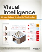
Joseph Priestly’s timeline of lifespan shown in Figure 11-1, is the earliest example of this form of chart, and it shows many of the key features that we still use today. Note the labeled timeline—running from 600 BC to 0 AD. The length of the line between the birthdate and the date of death of each man shown on the chart offers an easy way to see the lifespan of each.
Figure 11-1: An early timeline chart created by Joseph Priestly
A timeline has a graphic—a bar or a line—to show the start and end dates of an event or series of events. Timelines are useful in instances where you do not need to show a metric but rather a sequence of events, using the length of the line to delineate the length of time that has passed and showing qualitative metrics. Sometimes the qualitative metrics can include great detail, especially in an interactive version of the timeline is available where detailed write-ups of the event can be expanded.
Timelines are visually very similar to both bar charts and Gantt charts. Which chart is used depends on the context. Timelines are used primarily where no other data points are being shown, and qualitative data, such as the names of people or battles, need to be highlighted. Bar charts are used where additional data need to be shown, for instance using the color of the bar to distinguish between different processes. Gantt charts are used to display dependencies in the process on the timeline.
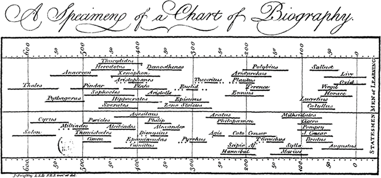
Figure 11-2: Another great example of the timeline is at the Imperial War Museum in London, in the bunker—this timeline runs from bottom to top, and interactively allows one to drill down into greater detail of events.
Ease of Development
| Reporting Tool | Predefined Chart Type | Ease of development |
| Excel | No | |
| PerformancePoint | No | |
| Power View | No | |
| Reporting Services | No | |
| Silverlight/HTML5 | N/A |
Line Charts
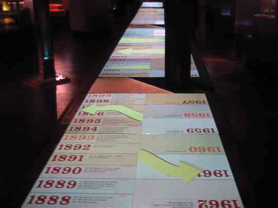
Line charts are a very simple way of showing a value by positioning data points on the vertical axis and drawing a line through the various points. If you plot different data points this way, the various lines are called series. The relative positioning of these lines enables you to easily make additional comparisons, as shown in Figure 11-3. This early example of a line chart by William Playfair shows a classic use of a line chart—comparing imports and exports over time, with the area of the chart between the lines being an important additional data point. Because the imports are additive over time, the overall area enables you to compare whether for the period as a whole, England has imported or exported more goods.
Figure 11-3: An example of an early line chart by William Playfair
Line charts are one of the most used and most useful chart types. They are present in almost every reporting tool, and they are used almost exclusively for showing changes over time. You must take care not to casually interpolate data between data points if the chart data is not contiguous. As an example, let’s consider a store that trades Monday to Saturday, and is closed on Sundays. If a chart for the month included Sundays on the axis, it would be misleading to draw a line from the sales value on Saturday to the sales value on Monday via Sunday, because the chart would then show a sales value for a day that the store was closed.
The area chart version of the line chart simply shades in the gaps between various lines on the chart. However, note that many of the challenges inherent in attempting to judge area are present in this type of chart.
Ease of Development
| Reporting Tool | Predefined Chart Type | Ease of development |
| Excel | Yes | |
| PerformancePoint | Yes | |
| Power View | Yes | |
| Reporting Services | Yes | |
| Silverlight/HTML5 | N/A |
Bar and Column Charts
Bar and column charts, as shown in Figure 11-4, are simply two versions of the same chart rotated 90 degrees. In a column chart the date is on the bottom axis. The additional series on the bar chart replaces the value used for the height on the column chart. However, the two charts are used very differently when it comes to temporal analysis. A bar chart uses the length of the bar to show a start and end date, with the position of the bar being the discrete item, whereas a column chart uses the length of the column to show a value. For temporal analysis, the date always runs from left to right. Some additional work is required in all the Microsoft tools to show the bar chart in the correct manner, as it has really been implemented as a column chart rotated 90 degrees. Figure 11-4 shows an example.
Figure 11-4: Bar and column charts are often confused, but the distinction is simple. Bars run from left to right, and columns from bottom to top.
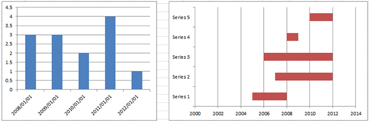
Both types of charts rely on the human eye being able to follow a straight line and make comparisons. It is always a good idea to add background lines to aid this process.
Ease of Development
| Reporting Tool | Predefined Chart Type | Ease of development |
| Excel | Yes | |
| PerformancePoint | Yes | |
| Power View | Yes | |
| Reporting Services | Yes | |
| Silverlight/HTML5 | N/A |
Combined Charting
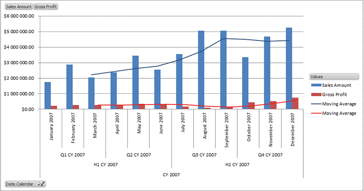
Using a line chart in combination with a column chart is one of the most powerful visualization techniques because it can be used either to show additional or derived data points, such as profit margin as a percentage against sales value or profit value, or it can be used to show a trend, such as a three-month moving average. Choice of color in this combined form is very important; if you have used multiple series that are differentiated by color, making sure that the line and the chart for matched series have similar colors is essential. Using different shades of the same color ensures that contrast is maintained between the line and the chart while still keeping the relationship clear. An example of using different shades of red and blue to match Sales Amount and Gross Profit to their moving averages is shown in Figure 11-5.
Figure 11-5: Using matched colors to show relationships between series
Ease of Development
| Reporting Tool | Predefined Chart Type | Ease of development |
| Excel | Yes | |
| PerformancePoint | Yes | |
| Power View | No | |
| Reporting Services | Yes | |
| Silverlight/HTML5 | N/A |
Scatter Plots and Bubble Charts
A scatter plot is a chart of points, graphed on an x and y (horizontal and vertical) axis. For static temporal analysis, the horizontal axis will be always be the time period of the chart.
A bubble chart is a refinement of the scatter plot. The horizontal position is still time, but in addition to using position on the vertical axis to represent a data point, the size of the bubble, its color, and, in some tools, its shape can be used to represent data points.
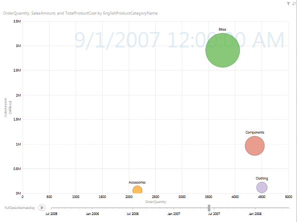
Bubble charts have been used with great effect as animated tools. Rather than showing time on the horizontal axis, another data point can be represented on the horizontal axis, and the changes over time are shown by changing the various values. The animation draws attention, as the bubbles grow or shrink, and move around on the plot. However, it is vital that the animation can be paused, and that the position on the timeline is shown, as shown in Figure 11-6.
Ease of Development
| Reporting Tool | Predefined Chart Type | Ease of development |
| Excel | Yes | |
| PerformancePoint | Yes | |
| Power View | No | |
| Reporting Services | Yes | |
| Silverlight/HTML5 | N/A |
Figure 11-6: A PowervView bubble chart
Tiling
Tiles are a series of similar charts, typically with one background filter applied to the charts in a series. In the context of temporal analysis, the background filter would be a discrete set of points in time, for example years or months. This is a technique that can be applied in Reporting Services with some amount of ease, by embedding a chart in a matrix, and PerformancePoint has the capability of doing this specifically for pie charts (the only possible advantage of having pie charts in PerformancePoint). However, the tool that truly shines with tiling is Power View, in which you simply drag a value to the Tile field to yield an exceptionally powerful visualization. The drawbacks of tiling are, of course, that much more screen real estate is needed when charts are repeated, and thus the charts themselves often end up smaller.
Ease of Development
| Reporting Tool | Predefined Chart Type | Ease of development |
| Excel | No | |
| PerformancePoint | No | |
| Power View | Yes | |
| Reporting Services | No | |
| Silverlight/HTML5 | N/A |
Animation
Animation in cinematic effects, for instance time-lapse filming, has always been an exceptional way to show how things change over time. Animation has only recently been used to good effect in the visualization field.
Many business intelligence (BI) tools have used animation to show transitions; it’s a nice visual effect, but it doesn’t add any value or informational content. Instead, using animation to show changes over time is an effective use of the tool. There are several different ways of showing changes over time. The most popular and information-dense method is in a scatter or bubble plot, in which the x- and y-axes, the bubble size, and the bubble color can be used to show dimension values or metrics. A visualization with these criteria is five-dimensional (x-axis, y-axis, the size of the bubble, the color of the bubble, and the animated changes)—very informationally dense.
A further enhancement is to combine tiling and animation, which allows for a better use of screen real estate. When you combine tiling and animation, you only show a few tiles and move them along to illustrate the change over time. You will see how to do this in the section “A Data-Driven Timeline Using Reporting Services” later in this chapter.
Ease of Development
| Reporting Tool | Predefined Chart Type | Ease of development |
| Excel | No | |
| PerformancePoint | No | |
| Power View | Yes | |
| Reporting Services | No | |
| Silverlight/HTML5 | N/A |
Tool Choices, with Examples
Temporal analysis is one place where all the Microsoft tools have strengths. However, PerformancePoint is the most limited, and Power View’s sole outstanding feature is animation.
PerformancePoint Services (PPS)
PerformancePoint supports column and line charts. When numeric values are combined with percentages, PerformancePoint automatically sets the chart type to a combined chart. Scatter plots, timelines, and animations are not supported at all.
The lack of a capability to combine line and column charts gratuitously is a serious hindrance, but PerformancePoint has another strength in temporal analysis in its internal awareness of the current date, and the ability to apply a formula to the date. The language used for this is called STP, short for Simple Time Protocol. After you have mapped a time dimension, STP allows for the addressing of dates. These will each be implemented either as connection formula or as formulas in a time intelligence filter.
Table 11-1 includes example formulae.
Table 11-1: STP Examples
| To display | Formula | Result |
| Yesterday | day-1 | The previous day relative to the current date. |
| Tomorrow | day+1 | The next day relative to the current date. |
| The current quarter and today | quarter, day | A set of time periods consisting of the current day and current quarter. |
| Last 10 days | day:day-9 | A 10-day range including today. |
| Last 10 days (excluding today) | day-1:day-10 | A 10-day range NOT including today. |
| Same day last year | (year-1).day | Current date (month and day) for last year. For example, if the current date were December 10, 2010, then (year-1).day would show information for December 10, 2009. |
| Same month last year | (year-1).month | Current month for last year. For example, if the current month were December, 2010, then (year-1).month would show information for December, 2009. |
| Same range of a period of six months last year | (year-1).(month-5): (year-1).(month) | From 18 months ago to one year ago. For example, if the current month were December 2010, then (year-1).(month-5): (year-1).month would show information for the time period ranging from June 2009 to December 2009. |
| Same range of months to date for last year | (year-1).firstmonth: (year-1).month | From the first month of last year up to and including the month parallel to the current month this year. |
| Year to date | yeartodate | A single time period representing the aggregation of values from the beginning of the year up to and including the last completed period. The period corresponds to the most specific time period defined for the data source. |
| Year to date (by month) | yeartodate.fullmonth | A single time period representing the aggregation of values from the beginning of the year up to and including the last completed month. |
| Year to date (by day) | yeartodate.fullday | A single time period representing the aggregation of values from the beginning of the year up to and including the last completed day. |
| Parallel year to date | yeartodate-1 | The aggregation of the same set of default time periods completed in the current year except for the prior year. |
Although all the examples in Table 11-1 are lowercase, STP is not case sensitive, and you may find that casing the formula elements makes them easier to read. For instance, instead of year, put Year, and use FirstMonth instead of firstmonth.
Examples of PerformancePoint column, line, and combined charts are included in Figures 11-7, 11-8, and 11-9.
Figure 11-7: A PerfomancePoint stacked chart showing a snapshot
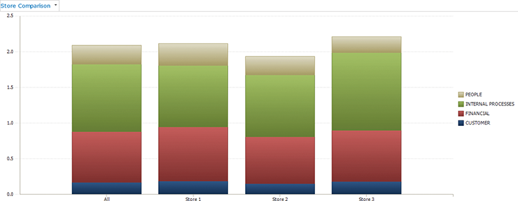
Figure 11-8: A PerformancePoint line chart
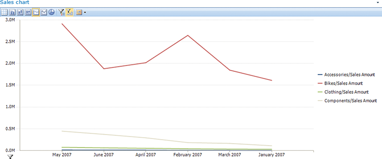
Figure 11-9: A PerformancePoint combined chart
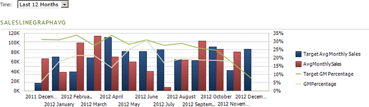
The combination of a Time Intelligence filter using STP formulae and a combined line and column chart is very powerful. In Figures 11-10 and 11-11 you can see how selecting a time period in the drop-down enables you to change the connected graph
Figure 11-10: A PerformancePoint chart filtered by an STP formula
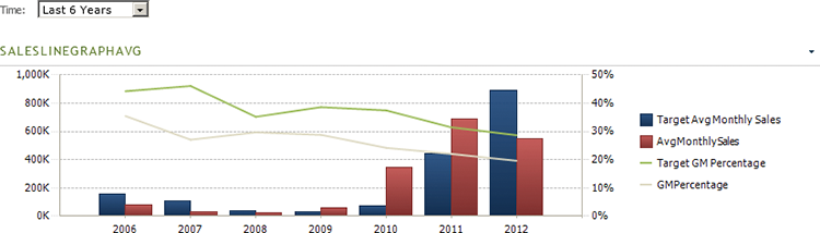
Figure 11-11: The same PerformancePoint chart filtered by a different formula
SQL Server Reporting Services (SSRS)
SQL Server Reporting Services (SSRS) enables you to have finely detailed control over the individual elements in the charts being displayed. SSRS supports line charts, column charts, combined line and column charts, bar charts, scatter plots, and—with a bit of ingenuity—timelines. The only visualization missing is the animation component.
Examples of SSRS column, line, and combined charts are shown in Figures 11-12, 11-13, and 11-14.
Figure 11-12: A column chart in Reporting Services
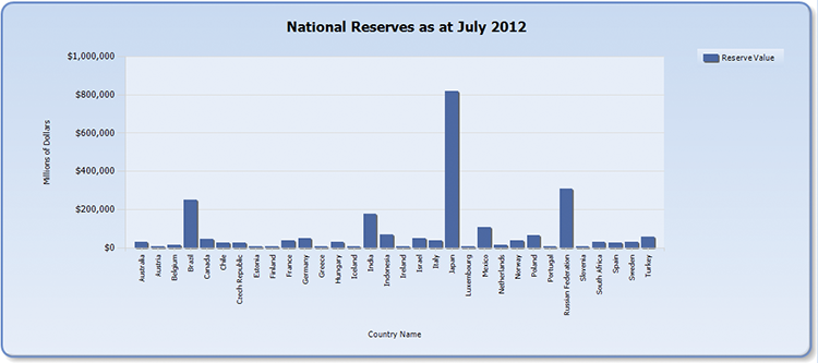
Figure 11-13: A line chart in Reporting Services
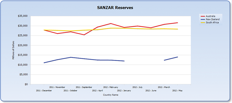
Figure 11-14: A combined chart in Reporting Services
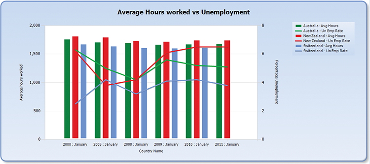
There are some issues with the default representation shown in Figure 11-14: notably that the gaps in the dates have been skipped, and the data set looks continuous when it is in fact not. This is a feature of SSRS to watch for.
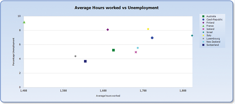
SSRS supports scatter plots natively, as illustrated in Figure 11-15. The default is to use different shapes for the markers, which is a nonstandard way of treating scatter plots. Some work with expressions is required to show the labels on the data points themselves.
Figure 11-15: A scatter chart in Reporting Services
A traditional bar chart is shown in Figure 11-16, and the slight modification to the chart to show as a timeline is shown in Figure 11-17.
Figure 11-16: A bar chart in Reporting Services
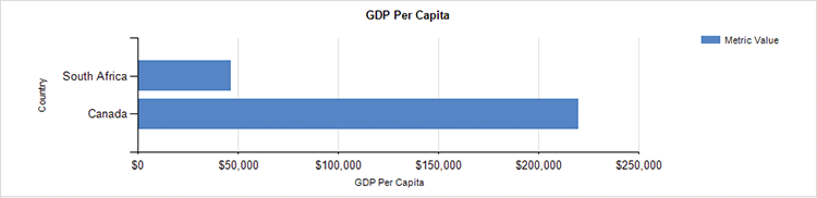
Figure 11-17: A Timeline in Reporting Services
Excel
Excel’s repertoire of line, column and scatter charts is very similar to SSRS when it comes to temporal charts. Although the timeline capabilities are missing, Excel has a very important addition known as trendlines, which are statistical extrapolations of the trend of the chart series to date.
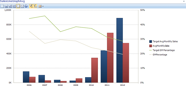
Examples of Excel column, line, and combined charts are shown in Figures 11-18, 11-19, and 11-20.
Figure 11-18: An Excel column graph

Figure 11-19: An Excel line graph
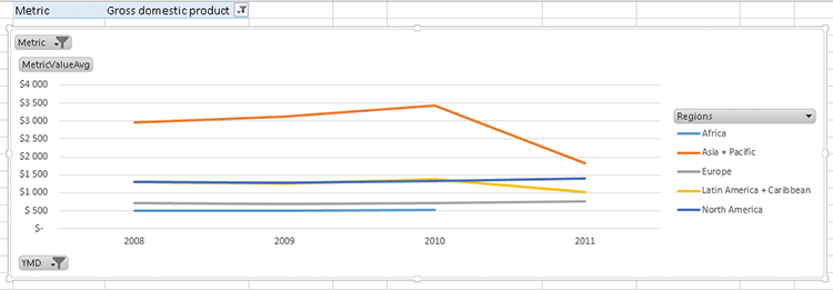
Figure 11-20: An Excel combined graph
The setup screen for the trendline is shown in Figure 11-21, and the resultant chart is shown in Figure 22.
Figure 11-21: Trendline options
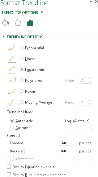
Trendlines can be calculated by various methods:
- Exponential: Showing a curved line, this trendline is useful when data values rise or fall at constantly increasing rates.
- Linear: Use this type of trendline to create a best-fit straight line for simple linear data sets. A linear trendline usually shows that something is increasing or decreasing at a steady rate.
- Logarithmic: A best-fit curved line, this trendline is useful when the rate of change in the data increases or decreases quickly and then levels out.
- Polynomial: This trendline is useful when your data fluctuates as happens, for example, when you analyze gains and losses over a large data set.
- Power: Showing a curved line, this trendline is useful for data sets that compare measurements that increase at a specific rate.
- Moving average: This trendline evens out fluctuations in data to show a pattern or trend more clearly. A moving average uses a specific number of data points (set by the Period option), averages them, and uses the average value as a point in the line
Figure 11-22: A column chart with trendlines
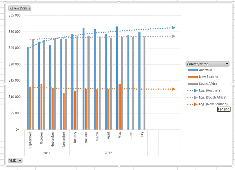
You have to add each trendline individually by right-clicking the series and choosing Add Trendline.
Power View
Power View has been designed for an interactive experience, and this truly makes it powerful for showing changes over time. The standard options for column, line, and bar graphs are all available in Power View. In addition, Power View enables both tiling and animation over time—truly a broad reach of visualization. The counterpoint to this, which is similar to PerformancePoint, is that there are limited customization options. Indeed, in terms of customizing how different components interact with each other, Power View has even fewer options than PerformancePoint.
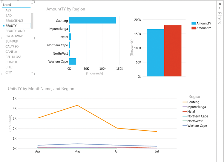
In Figure 11-23, you can see a combination of bar, column, and line charts that are being filtered by a single slicer. The time required to build a visualization like this is much less than PerformancePoint, SSRS, or even Excel, as the connections are all built behind the scene.
Figure 11-23: A Power View analysis page
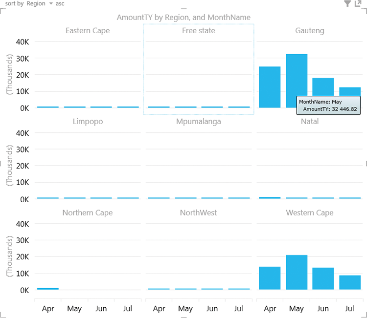
You experience the power of Power View (forgive the pun!) when you apply the newer features. For one thing, tiling (automatically repeating the same graph and filtering by a value, which is possible in SSRS, and is exceptionally hard work in PerformancePoint and Excel) is performed simply by dragging the tiled value into a box and having the tiles show up automatically. For a comparison over a discrete set of time values—for instance, months of the year—tiling is a great way to get a snapshot comparison, as shown in Figure 11-24.
Figure 11-24: Power View tiled charts
Power View also has an animated scatter plot feature. This feature can’t be used in combination with tiling, but is as easy to implement. Simply create a scatter plot chart and drag your date field to the Play Axis. The Play Axis is a slider along the bottom of the chart which can be used to set a point in time, or animate over the data points. Figure 11-25 shows a basic scatter plot, and Figure 11-26 shows—as much as is possible in a static image—the animation effects available. It is interesting to note how Power View shows the track of a particular data series over time when it is clicked upon—a very useful effect.
Figure 11-25: A scatter plot with the animated Play Axis at the bottom

Figure 11-26: A Play Axis tracing the positions and sizes of the bubbles

Implementation Examples
The implementation examples in this section use the OECDPopulation PowerPivot model available from this book’s web page (www.wiley.com/go/visualintelligence), and called OECDPopulationStats.xlsx. Building the model is covered briefly in the next section, but refer to Chapters 5 and 6 for more details.
Power View Animated Scatter Plot
Power View’s best feature is the animated scatter plot. With a focus on interaction in general, the ability to drag a slider to animate changes in time (or just let it play), this visualization is Power View’s raison d’etre. In this section you learn how to implement it.
Building a Model to Support Power View
Please see Chapters 5 and 6 for an introduction to building a PowerPivot workbook. This section requires at least Excel 2010 for the PowerPivot pieces, and Excel 2013 for Power View.
Power View requires a PowerPivot (or tabular) model to support the animation. You will need to set up a date table to allow the animations to work correctly. Create a connection to the VI_UNData database, and make sure you have imported the DimDate view, and the DimCountry, DimOECDStatistic, FactOECDNationalReserve, and FactOECDPopulation tables. Note that the DimDate view is near the bottom, and don’t choose the DimDate table. Your sheet should look similar to Figure 11-27.
You need to set up the relationships to the DimDate view by first clicking the diagram button in the bottom right, and then creating relationships from the two fact tables to the DimDate, using DimDateID. You need to click on the DimDateID field on the fact table, and dragging it onto the DateID field on DimDate. Your diagram should look like Figure 11-28.
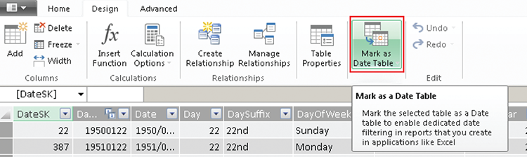
Right-click DimDate, and choose Go To which will take you to the table designer. In the Ribbon at the top, choose the Design tab and click the Mark as Date Table button, as in Figure 11-29.
Figure 11-27: Initial model setup
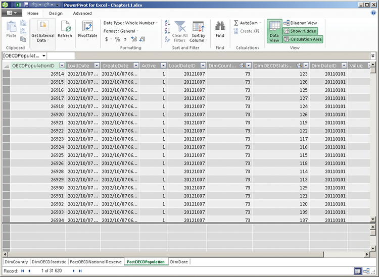
Figure 11-28: The PowerPivot diagram designer
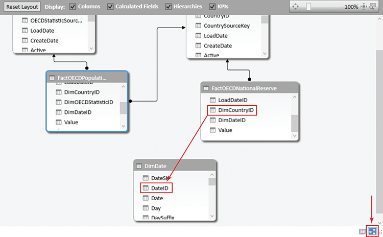
Figure 11-29: Marking a table as a date table
Click OK in the next window. You need to fix up the sorting of the Month names by selecting the Month name column, and clicking Sort by Column on the Ribbon’s Home tab. Choose MonthNumber, as in Figure 11-30.
Figure 11-30: Sort by columns
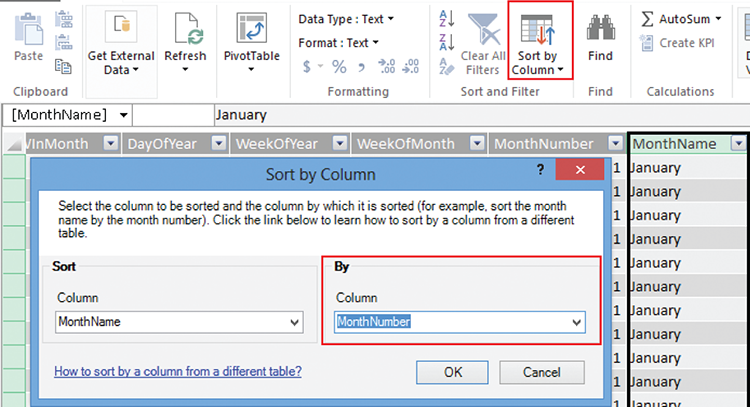
Repeat the process for MonthNameFull.
Next, you need to set the row identifier. The row identifier is similar to the primary key in SQL Server, and is a number that uniquely identifies each row. Start by enabling the advanced tab. This option is found under the file menu, and is called Switch to Advanced Mode. Change to the Advanced tab, click Table behavior, then select OECDPopulationID in the drop-down box for the row identifier. Click the OK button.
Your final step is to create some measures that you are going to use in the scatter plot. You need to create a measure for each dimension value you are going to analyze. The three to analyze are Average Hours Actually Worked, GDP per Capita, and GDP per Hour Worked.
Create each of these on the FactOECDPopulation table, and use the following formulae:
AvgHours:=CALCULATE(
AVERAGE(FactOECDPopulation[Value])
, DimOECDStatistic[Metric]  = "Average hours actually worked"
)

GDPPerHour:=CALCULATE(
AVERAGE(FactOECDPopulation[Value])
, DimOECDStatistic[Metric]  = "GDP per hour worked"
)

GDPPerCapita:=CALCULATE(
AVERAGE(FactOECDPopulation[Value])
, DimOECDStatistic[Metric]  = "GDP per capita"
)
You will do this by right-clicking Add Column. Rename the column to AvgHours. Paste the formula, starting with the equal sign, into the formula bar making sure to keep all the text of the formula on one line.
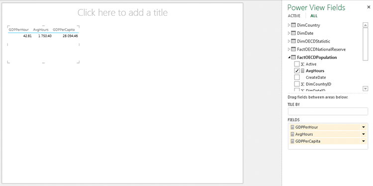
Save your workbook. Now that you have a Power View model, you are going to build out the animated scatter plot. Start by going back to Excel and clicking Power View on the Insert tab. On the new sheet that is created, drag GDPPerHour, AvgHours, and GDPPerCapita (in that order) from FactOECDPopulation in the field choice tab on the right to the value box, as shown in Figure 11-31.
Figure 11-31: Dragging fields to the value box
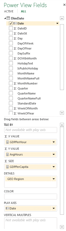
Change the chart type to a scatter plot (you do this in the Design tab, under Other Chart). Resize the chart to fill the screen. Drag GeoRegion from DimCountry to the Details box on the right side, and drag Date from DimDate to the Play Axis box (see Figure 11-32).
Figure 11-32: Power View field choices
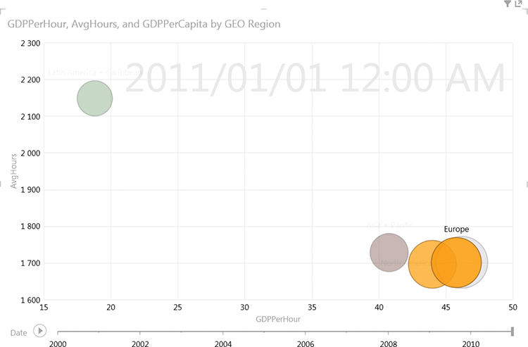
The result is an animated scatter chart, which you can play; alternatively, you can drag the slider to see data at a point in time. If you click a particular data item, you see the history for that item. Figure 11-33 shows an animated bubble chart.
Figure 11-33: A Power View bubble chart
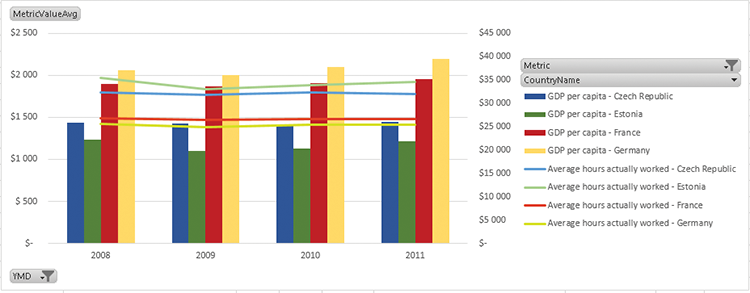
Combining Lines and Columns in Excel
In this section, you are going to track the relationship of Gross Domestic Product to population size over time. This example uses Excel 2013, which has a combined chart type that makes this process easier, but in earlier versions of Excel it is easy enough to simply change one of the chart series types to a line chart to create a combination chart.
Switch to Sheet 1, then start by clicking the Pivot Chart button on the Insert Ribbon, as shown in Figure 11-34.
Figure 11-34: Excel Ribbon interface to add a pivot chart
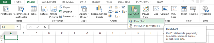
Figure 11-35: Choosing a connection for a pivot chart

Choose Existing Worksheet and Use an External Data Source. Click Choose Connection, as shown in Figure 11-35.
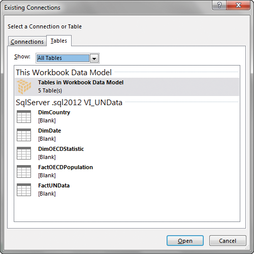
The choice of a connection is a bit different between Excel 2013 and earlier versions. In the earlier versions, you select PowerPivot as the data source, but in Excel 2013 you must choose Tables and then select Tables in Workbook Data Model, as shown in Figure 11-36.
Figure 11-36: Choosing a connection in Excel 2013
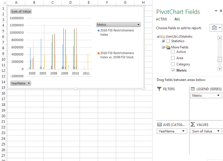
At this point, you see an empty pivot chart on the left and the PivotChart Fields pane is on the right, but you need to add the appropriate fields to the chart. Start by adding the Value field from the FactOECDPopulation table to the Values block, and Metric from DimOECDStatistics to the legend, and YearName from DimDate to the Axis, as shown in Figure 11-37.
Figure 11-37: An Excel pivot chart
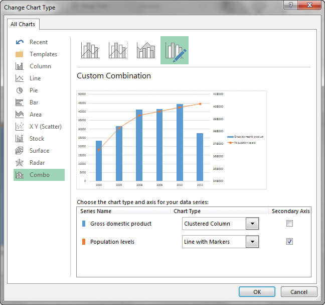
At this point, the chart isn’t showing anything meaningful for analysis, just a selection of the metrics. Start narrowing down the selection by clicking Metrics in the pivot chart and selecting Gross Domestic Product and Population Levels. This restricts your data set to the values you want to compare. However, to compare them you need to format them to show a line and a column, and you need to set up secondary axes. In Excel 2010 and earlier, you do this by changing the chart series type individually, but in Excel 2013 if you right-click anywhere on the chart and select Change Chart Type, you are presented with the new chart selector window, as shown in Figure 11-38.
Set the chart type to Combo, and select Secondary Axis for Population levels. Click OK.
Figure 11-38: Changing a pivot chart type
This chart is a great showcase of one of the biggest fallacies in temporal analysis—points on the axis that have no data are hidden (for example Monday being followed by Wednesday because Tuesday had no data), thus altering the slope of the curve.
To fix this issue, you need to make several changes: Show the missing data points, limit the chart to the relevant dates, and add a trendline to interpolate the missing years.
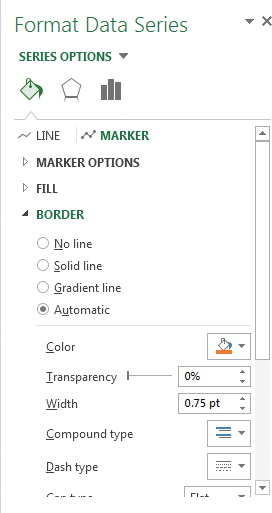
To add the missing data points, right-click the chart area, and click PivotChart Options. Choose the Display tab, select the Show Items with No Data on Axis Fields option, and then click OK. All the years are now displayed, and you filter them by clicking YearName and choosing the years 2000 through 2012. The gross domestic product series is showing correctly as columns, but you need to add markers for the line chart to show noncontiguous values. Right-click the line and choose Format Data Series. If you’re using Excel 2013, you should see a pane like the one in Figure 11-39; in earlier versions of Excel, you see pop-up window. Click the Paint icon, then choose Marker, and choose a series marker in Marker options—the default Square and size 5 will work nicely—and show the values of Population levels on the chart.
Figure 11-39: The Format Data Series pane in Excel 2013
The final piece to this chart is showing interpolated values. This is where Excel truly shines over the other tools. Right-click on the line chart, and click Add Trendline—all the default values are fine (although you may want to play with the forecast feature!). Click OK. You see the final chart shown in Figure 11-40. You would, of course, finish off by formatting the axes appropriately.
Figure 11-40: An interpolated population chart

A Drillable Line Chart in PPS
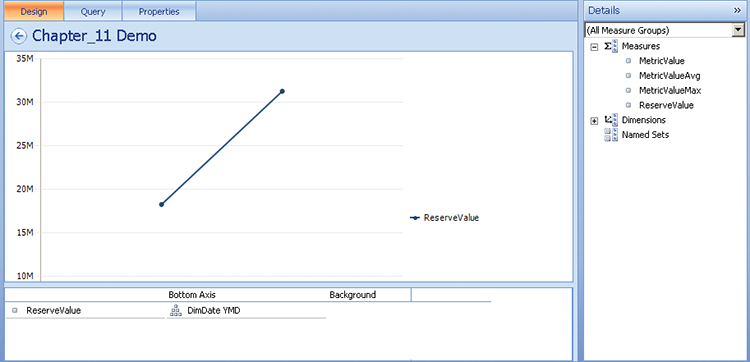
In PerformancePoint, set up a data connection as described in Chapter 7, making sure to set up the time dimension correctly. You use the OECD_Data model that you setup in Chapter 7, and create an analytic chart. Right-click the library and click New > Report. Choose Analytic Chart and then choose the data source you created. In the chart design screen, drag the YMD hierarchy from DimDate into the Bottom Axis column. Drag ReserveValue from Measures into the series. Finally, right-click the chart and select Report Type > Line Chart with Markers.
To choose the appropriate data, click the All value on the bottom axis and then right-click next to it so you can select Filter > Filter Empty Axis Items. At this point, you see a chart such as the one in Figure 11-41.
Figure 11-41: A PerformancePoint analytic chart
Once deployed, this chart is automatically drillable by clicking on the year to drill down to the months. You can create additional time series by using time intelligence filters. In order to make it interactive with the other components of PerformancePoint you need to add other dimensions to the background.
A Data-Driven Timeline Using SSRS and Data Bars
SSRS can do all the visualizations that you have worked with so far this chapter barring the animation, but it also has the capability of doing a timeline. This isn’t a standard visualization in SSRS, but it is relatively easy to do. You use Report Builder to build the report, as described in Chapter 8. Start by creating a data source connection to the OECD_Data tabular cube in Report Builder and then creating a new data set.
To do so, open Report Builder and you will see the Getting Started Wizard. Click on Chart Wizard, then click Next on the following screen. Click New to create a new data source, then choose Microsoft SQL Server Analysis Services from the Select connection type drop-down, and enter rsds_OECDDatain the Name text box (this could be any name).
Click the Build… button. If you are using a local and unnamed Analysis Services instance, you can just enter “.” in the Server name box, otherwise enter the server you are connecting to. Finish off by choosing OECD_Data for the database name, and clicking OK. Click OK again and then click Next to create the data set.
In this data set, filter by the GDP per Capita metric, and add the YMD hierarchy, the Country Name hierarchy, and the MetricValue measure to the design surface, as shown in Figure 11-42. Add the DateSK column—this is an incrementing column that starts at 1 for the first date and has no gaps. It’s ideal for calculating distances on a chart.
Figure 11-42: The Reporting services data set designer
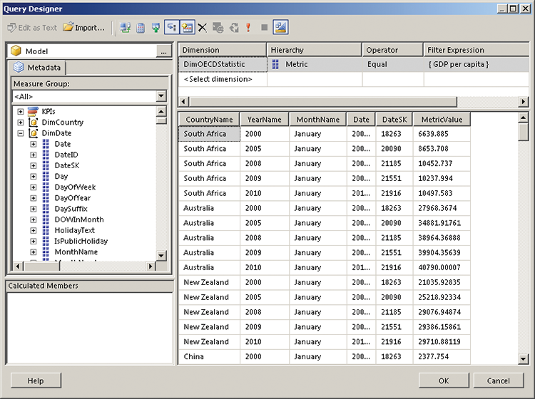
This data set is going to be too large to work with easily, so filter it just for South Africa and Canada. You do this by dragging CountryName onto the filter pane at the top on the right, and then choosing South Africa and Canada from the drop-down. Click OK twice to close the designer when you’re done.
You’re just working on the chart, so remove the titleand footer from the report. You remove the title by clicking on it, and then hitting the Delete key, and you remove the footer by right clicking on it and choosing Remove footer.
Click the Chart option on the Insert tab, choose Chart Wizard, and in the window that displays select the data set you just created. Click next. Choose Bar, click Next, and then enter CountryName into the Categories and DateSK into the values column. Click the arrow next to the DateSK and choose Max as the aggregation value.
On the next screen choose the Generic style and then click Finish.
When the chart appears on the report design surface, drag the bottom-right corner to make the chart big enough to show all the values and then right-click the chart and click Change Chart Type. Scroll to the bottom to find the Range category. Choose the Range Bar chart type (it is fourth from the left).
Click the Low value that appears on the right side, and change it to use the DateSK field and to aggregate as Min, as shown in Figure 11-43.
Figure 11-43: Setting the DateSK field to aggregate as Min

Format the chart by right-clicking near the vertical axis (around the CountryName labels). The words CountryName are repeated down the left hand side, next to the words Axis title, and you need to click between two of the lines containing CountryName. Then choose Vertical Axis Properties. Set the interval to 1 from Auto to show all the countries. Set the Axis title at the same time.
Next, right-click the bottom axis and select Horizontal Axis Properties. Deselect the Always Include Zero button. Set the minimum value to 18232 (This is the value of the first key in the data set, minus 30, to set the chart to display data points prior to the start of the data set), and the maximum to 22281 (this is the value of the last key in the data set), set the interval to 12, and then set the interval type to Months. Set the Axis title at the same time. On the same screen there is a text box for the Axis title, which will replace the words “Axis title” displayed previously. Make the axis title Country.
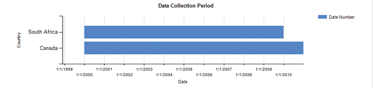
Run the report by clicking the Execute button and you see a display similar to Figure 11-44.
Figure 11-44: Running the report
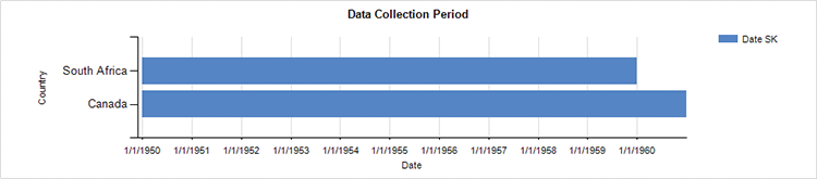
It’s immediately apparent that the dates are wrong. This is because the data set uses 1950/01/01 as the base date, and a date type in SSRS is based upon a date starting in 1900/01/01. If you create a new calculated field in which you add 18262 to the DateSK and then add 18262 to the minimum and maximum values, you get a chart such as that shown in Figure 11-45, which shows an accurate timeline for when data was collected for South Africa and Canada:
Figure 11-45: Date ranges displayed in SSRS

Summary
In this chapter you learned about using visualizations to present data that changes over time, and the pitfalls to avoid. The different tools in the Microsoft stack are all good at displaying temporal data, but for different purposes: PerformancePoint is good with custom date ranges, Power View has an animated bubble chart, Excel has trendline functionality, and Reporting Services can display timelines with ease.