
Optimizer
Abstract
The Optimizer is used on existing working analog circuits to improve performance by optimizing component values or system parameters. Optimizer specifications are set using either Measurement definitions to determine circuit performance by varying circuit parameters or by using Curve-fit definitions that are applied to the profile of the output waveform. Circuit performance is evaluated using measurement expressions from transient, DC, or AC simulations, applied to the circuit output waveforms. Goal functions and constraints are then used to define circuit specifications to optimize circuit performance against measured values for a change in defined parameter values. Goal functions set “loose” target specifications that would be nice to achieve, whereas constraints set limits to which the output of the measurement expressions aim to achieve by a series of optimization steps.
Keywords
Performance; Optimizer; Goal function; Waveform; Circuit; Curve-fit
Introduction
The Optimizer is used on existing working analog circuits to improve performance by optimizing component values or system parameters. Optimizer specifications are set using either Measurement definitions to determine circuit performance by varying circuit parameters or by using Curve-fit definitions that are applied to the profile of the output waveform. Circuit performance is evaluated using measurement expressions from transient, DC, or AC simulations, applied to the circuit output waveforms. Goal functions and constraints are then used to define circuit specifications to optimize circuit performance against measured values for a change in defined parameter values. Goal functions set “loose” target specifications that would be nice to achieve, whereas constraints set limits to which the output of the measurement expressions aim to achieve by a series of optimization steps.
Once the measurement expressions for circuit performance have been identified, you then need to define your goals or constraints that will improve circuit performance. Running a sensitivity analysis will give an indication as to which parameters have the most significant effect on circuit performance. These parameters are then imported from the results of the sensitivity analysis or can be imported directly from the circuit diagram. Component parameters are automatically set having maximum and minimum values at a factor of 10 times the nominal value. However, the values of these limits can be changed.
25.1 Optimization Engines
There are three optimization engines, the Modified least square quadratic (LSQ) engine, the Random engine, and the Discrete engine. The Modified LSQ engine is a fast gradient-based engine and is used to quickly converge to an optimum solution. However, if the optimizer gets mathematically “stuck” in what is called a local minima, then the Random optimization engine is used as it can provide alternative starting points. After an optimum result has been achieved, the Discrete engine is used in conjunction with discrete tables of commercially available passive component values to provide a realistic circuit in terms of practical component values.
The efficient use of the optimization engines depends on many factors such as how the circuit behaves, the number of circuit parameters to optimize, the range of the constraints and goals, and even the number of goals and constraints. It would be sensible to minimize the number of parameter variables initially to get a feel for how the optimizer is progressing toward the optimum specifications.
25.2 Measurement Expressions
Measurement expressions return single numerical values from an output waveform as a measure of circuit performance; for example, rise time, low pass cut off − 3 dB, or a user-defined “value.” The single value returned can be that of a single point trace function x-y value, a measurement expression based on a combination of functions or a user-defined optimizer expression.
25.3 Specifications
Circuit specifications consist of a measurement expression and a defined goal or constraint. There must be at least one goal function defined in the list of measurement expressions. For example, a circuit has been designed to deliver a rectangular current pulse of up to 1 mA with a pulse duration of 100 ms ± 5% and a pulse period 500 ms ± 5%. The Max Measurement expression can be used to measure the maximum current and since a range has not been specified, this can be set as a goal function. A Period Measurement Expression can be used for the 100 ms pulse width with constraint limits of 95–105 ms. Similarly a period measurement can be used to determine pulse period with constraint limits of 475 and 525 ms.
The progress of a measurement for a specification compared to other specifications can be emphasized in the error graph by setting up a weighting function that effectively scales up the error at each data point. For example, say you have five specifications defined. As the weight function integer is set by default to 1, each specification will contribute 20% to the total error at the start of the optimization regardless of the initial error margin from goal or constraint ranges. If you prioritize one specification, specification A, with a weight of 6 leaving all other specification weights set at 1, then the total contribution to the specification A is (6 + 1 + 1 + 1 + 1) = 10. Specification A will then contribute, 6/10 × 100 = 60% to total error at the start of optimization with all other specifications contributing 10%. In the error graph, you can see the progress of the optimization measurements and any effects a weighted specification has on measurements converging to a final solution.
The idea of the optimization process is to reduce the difference or error between a calculated measurement and defined goals or constraints by varying component parameters. The error graph gives an indication of the progress of the optimizer to converge toward a solution that meets the specified goals and constraints and also provides a history of the simulation data. The error is determined using the process of least mean squares and is displayed as normalized % error against the number of runs. The error calculation is based on

where
MEc—difference between current measurement value and nearest edge of desired range (i.e., constraint).
MEo—difference between original measurement value and nearest edge of desired range.
W—weighting integer.
Σ—sum of weighted integers.
Exercise 1
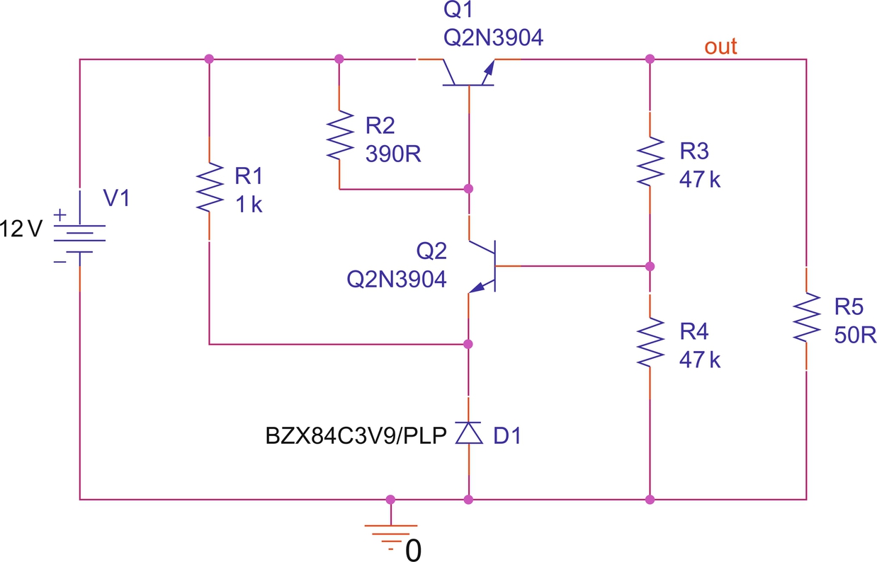
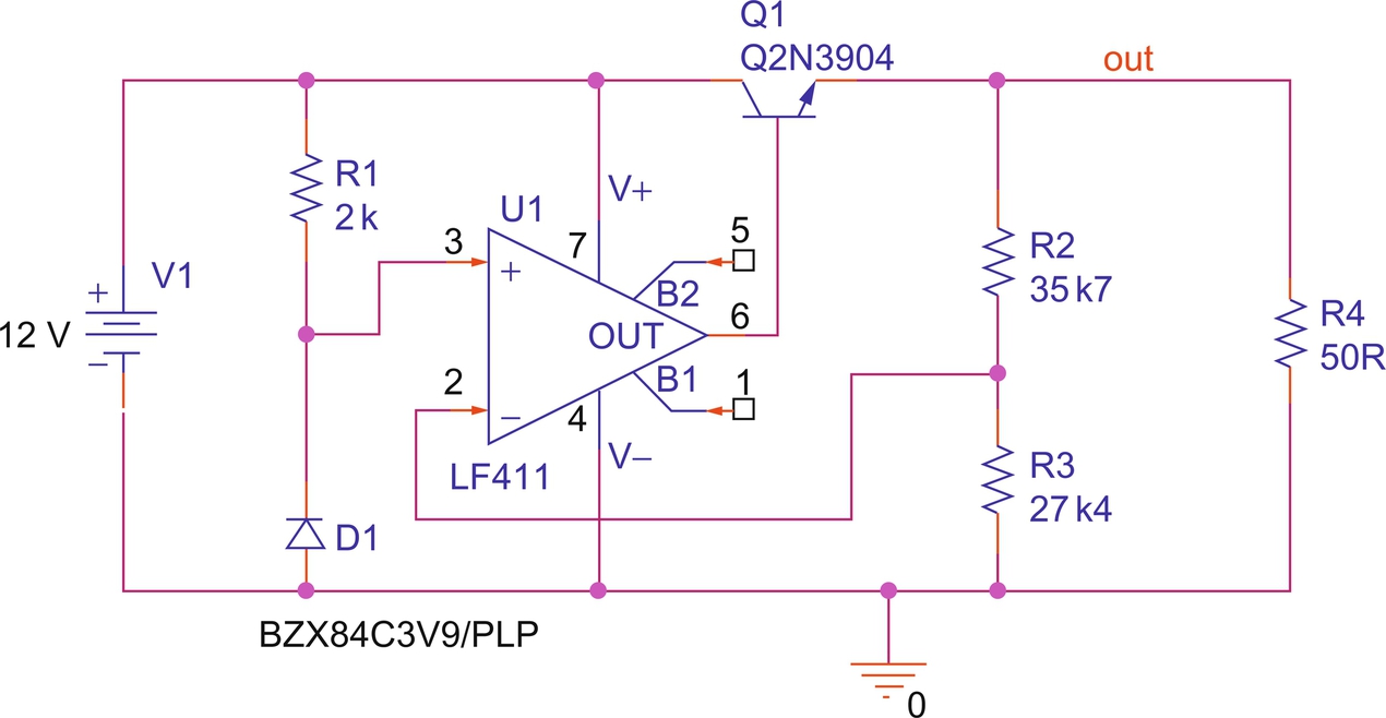
Following on from the results of the sensitivity analysis in Chapter 24, the power supply circuit performance will be optimized for R1, R2, and R3. The circuit diagram is shown in Fig. 25.1.
1. Open the voltage regulator circuit from the Sensitivity analysis in Chapter 24.
2. Highlight Q1 and rmb > Edit PSpice Model and delete the dev = 50% and leave Bf = 200.
3. Run a transient analysis using the default Run To Time of 1000 ns.
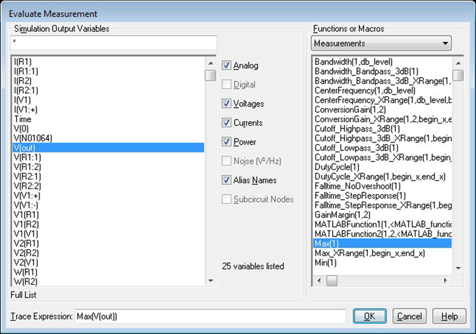
4. Measurement Expressions were set up in Sensitivity analysis and can be seen in PSpice, View > Measurement Results. If the expressions were not set up, then select Trace > Evaluate Measurement that will open up the Evaluate Measurement window. Select Max(1) from the Functions and Macros list and then select V(out), see Fig. 25.2. Click on OK.
5. Create another Measurement Expression using the Max function for the current through R4, Max(I(R4).
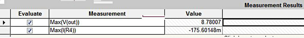
6. In PSpice select View > Measurement Results and click on the Evaluate to see the measurement results (Fig. 25.3).
7. In Capture select PSpice > Advanced Analysis > Optimizer.
8. In the Parameters [Next Run] window, click on, Click here to import a parameter from the design property map….
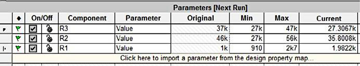
9. In the Parameters Selection Component Filter [⁎] window, hold down the Control Key and select R2 Value, R3 Value, and R4 Value. The parameters will appear as shown in Fig. 25.4.

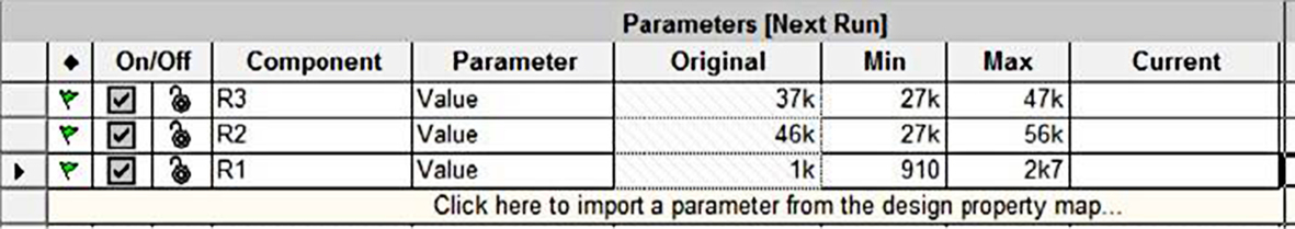
10. Component parameters are automatically adjusted to a decade either side of nominal value. Change the parameter ranges to that shown in Fig. 25.5.
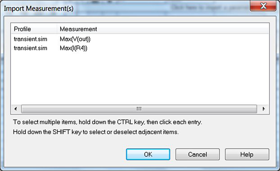
11. You need to set up the Measurement Specifications. Click on, Click here to import a measurement created within PSpice…. You should see the two previous Measurement Expressions as shown in Fig. 25.6. If not, open PSpice and select View > Measurement Results and make sure the Evaluate button is checked for both measurements.
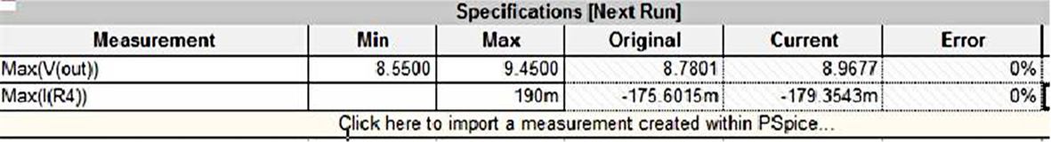
12. The circuit specifications are Vout = 9 V ± 5% and I(R4) = 190 mA. So Vout will be constrained between 8.55 and 9.45 V and I(R4) will be set as a goal. In the Specifications [Next Run], for Max(V(out)), enter a Min value of 8.55 and a Max value of 9.45. From the Type pull down menu, change Goal to Constraint. Leave the Weight as 1.
13. For Max(I(R4)), enter a Max value of 190 m and leave the Type as Goal. Change the Weight factor to 3 (see Fig. 25.7).

14. From the top tool bar, the Modified LSQ engine will be shown by default. Click on the run button.
15. You should see the optimized results shown in Fig. 25.8.
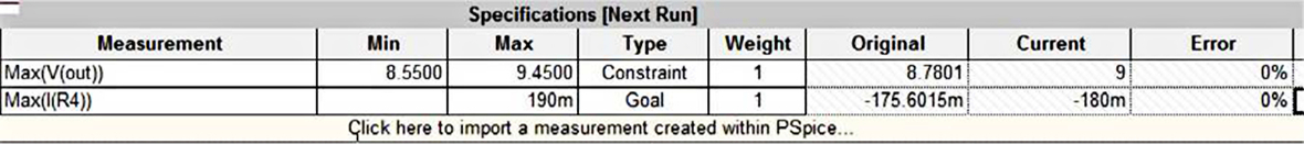
The minus sign in front of the original − 175.6015 mA refers to the direction of current flow associated with pin 1 of resistor R4. By convention, current flow into pin 1 is positive. When you place R4 in the circuit and rotate once, pin 1 is at the bottom of the resistor so current flows out of pin1 and is recorded as negative.
16. The results in the Parameters [Next Run] (Fig. 25.9) show that the current component values that are not commercially available.
17. From the top tool bar, select Edit > Profile Settings to open the Profile Settings window and select Discrete from the Engine pull down menu. Click on the square-dotted ion next to the red cross, New (Insert) as shown in Fig. 25.10. If the discretetables esistance folder is not shown, then click on the three ellipses (…) and navigate to the discretetables esistance folder that can be found in, < install path > oolspspicelibrarydiscretetables esistance.
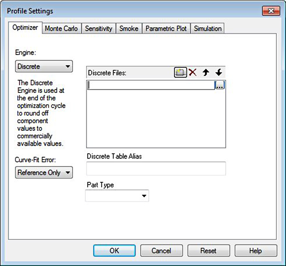
18. Select the res1%.table and in Part Type, select Resistance from the pull down menu, see Fig. 25.11. Click on OK to close the Profile Settings window.

19. Change the Modified LSQ engine to the Discrete engine from the pull down menu.
20. In the Parameters [Next Run] window, click in the Discrete Table box for R4 and from the pull down menu, select Resistors—1%. Repeat for R3 and R2, see Fig. 25.12.

21. Rerun the Discrete simulation.
22. Fig. 25.13 shows the specification results.
23. Fig. 25.14 shows the discrete 1% resistor parameter values.

24. Right mouse click in the Error Graph and the cursor will appear. Move the cursor to previous Run Numbers and you will see the Current results and Error change based on previous Measurement data.
25. Right mouse click in the Error Graph and select Clear History.
26. Change the simulation engine to Random and run the simulation. You should see similar results but bear in mind you still have to run the Discrete engine.
27. Replace the resistor values for R1, R2, and R3 with the 1% resistor values and re-run the PSpice transient simulation to confirm the optimized circuit outputs. For circuits with a large component count, a useful feature is to rmb on a resistor and select Find in Design.
The revised resistor values will be used for the Monte Carlo analysis and Smoke analysis.
The optimized power supply circuit is shown in Fig. 25.15.
Exercise 2
Curve fitting can be used to optimize model parameters to match characteristic graphs from datasheets or from empirical measured data. Curve-fit definitions can also be applied to the profile of a circuit's output waveform that is measured against a reference waveform where single data points can be measured using the trace expression, YatX. A curve fit specification consists of a reference file of measured data points and a corresponding measurement. Optimizer specifications are set using measurement expressions to determine circuit performance by varying circuit parameters. Circuit performance is evaluated using measurement expressions from transient, DC, or AC simulations, applied to the circuit output waveforms.
1. File > Open > Demo Designs and select the Optimization using Curve-Fitting design.
2. The circuit is that of a 4-pole low pass filter.
3. An AC logarithmic sweep from 100 Hz to 1 kHz has been set up.
4. Run the simulation and you will see the magnitude and phase response waveforms for the circuit.
5. From the top tool bar, select PSpice > Advanced Analysis > Optimizer. The Optimizer should be set up as shown in Fig. 25.16. Select the Curve Fit tab if not already selected.
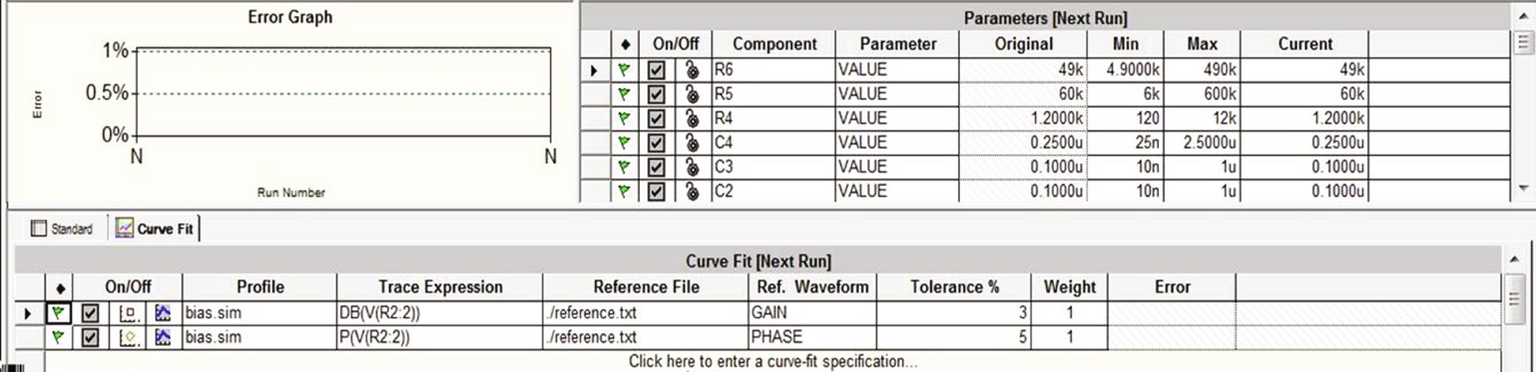
6. The Trace Expressions have been set up to measure the magnitude in dB and phase of the filter output. The reference file is a text file that contains waveform data for the required magnitude and phase responses of the filter.
7. Click once in the /reference.txt box and then click on the square icon with three ellipses. This will open up a window showing the contents of the Schematic 1 folder; ac and bias folders and the reference file.
8. Select the reference file and rmb > Open with > Wordpad. The reference file contains data columns for Frequency, Phase, and Gain. Close Wordpad and Cancel the Open window.
9. The Ref. Waveform fields incorporate a pull down menu that lists the GAIN and PHASE names from the reference file. The tolerance value is used in conjunction with the method for error calculation using optimizer parameters known as Gears that is set in Profile Settings under Curve-Fit Error. From the top tool bar, select Edit > Profile Settings > Optimizer.
10. Close Profile Settings.
11. More information regarding Gears can be found in the PSpice Advanced Analysis User Guide.
12. Make sure the Modified LSQ engine is selected and run the Optimizer simulation. You should see two curves in the Error Graph, one for gain and one for phase. The results of the simulation show that optimization has been achieved. The optimized component values are shown in the Parameters [Next Run] window pane (see Fig. 25.17).

13. Go back to PSpice and you will see the optimized curves displayed for gain and phase.