
Transformers
Abstract
A transformer is implemented by magnetically coupling two or more coils (inductors) together. For air core transformers, a K_Linear coupling device from the analog library is used, whereas for nonlinear transformers, a magnetic core model is referenced by the K coupling device. When creating a linear transformer, the coils are specified in units of henry (H), whereas for nonlinear transformers, users specify the number of turns for the inductors. The PSpice magnetic cores model hysteresis effects and include a coupling coefficient, which is used to define the proportion of flux linkage between the coils. A step-down linear transformer is presented using inductors for the primary and secondary windings which are specified in Henry's. Ideally, the primary and secondary circuits are electrically isolated. However, for PSpice simulation, there must be a DC path to ground for every node. A circuit for a nonlinear transformer created using three inductors for the coils, L1, L2 and L3 is presented. The reference designators, L1, L2, and L3, are added to the K device in the Property Editor and displayed on the schematic to indicate which coils make up the transformer. A linear transformer is available in the analog library. Nonlinear transformers, which include center-tapped primary and secondary windings, can be found in the breakout library. These transformers have properties that enable users to enter the inductance, coil resistances, and number of turns.
Keywords
Linear; Transformer; Coefficient; Flux linkage; PSpice; Coils
A transformer is implemented by magnetically coupling two or more coils (inductors) together. For air core transformers a K_Linear coupling device from the analog library is used whereas for nonlinear transformers a magnetic core model is referenced by the K coupling device. When creating a linear transformer the coils are specified in units of henry (H) whereas for nonlinear transformers you specify the number of turns for the inductors.
The PSpice magnetic cores model hysteresis effects and include a coupling coefficient which is used to define the proportion of flux linkage between the coils and has a value between 0 and 1. For coils wound on the same magnetic core, the coupling coefficient has a value almost equal to 1. For air cored coils, the flux linkage is smaller.
9.1 Linear Transformer
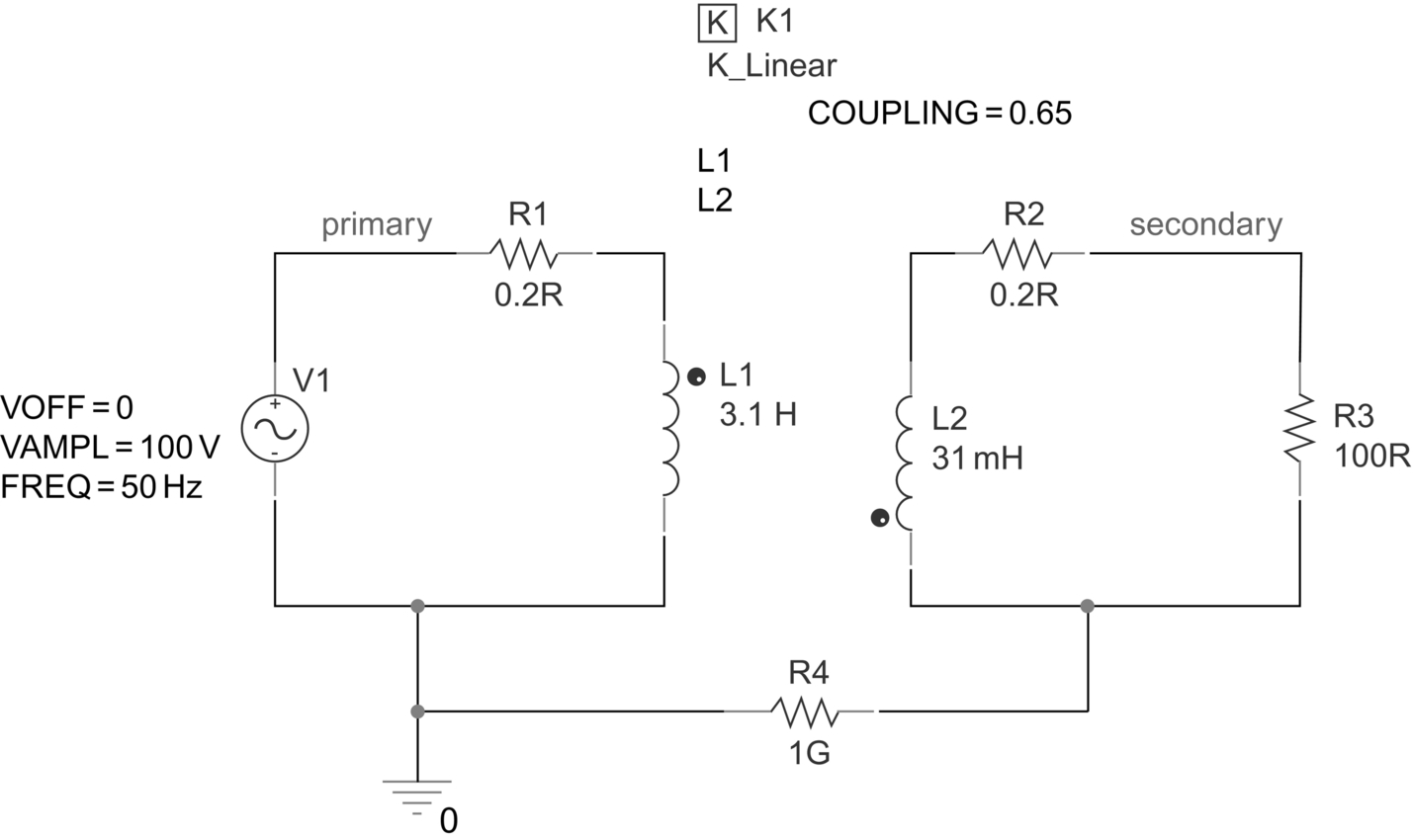
Fig. 9.1 shows a step-down linear transformer using inductors for the primary and secondary windings which are specified in Henry's. The two coils are magnetically coupled together using the K_Linear part, K1, which shows that L1 and L2 are coupled together. Ideally, the primary and secondary circuits are electrically isolated. However, for PSpice simulation, as mentioned in Chapter 2, there must be a DC path to ground for every node. This is achieved by using a large value resistor R4 connected from the secondary to 0 V, which will not have a significant effect on the accuracy of simulation.

9.2 Nonlinear Transformer
Fig. 9.2 shows a circuit for a nonlinear transformer created using three inductors for the coils, L1, L2 and L3. The reference designators, L1, L2 and L3, are added to the K device in the Property Editor and displayed on the schematic to indicate which coils make up the transformer. The standard K coupling devices allow for up to six inductors to be coupled together. Manufacturer's magnetic core models are found in the magnetic library. In this example, the E13_6_6_3C81 magnetic core is used.
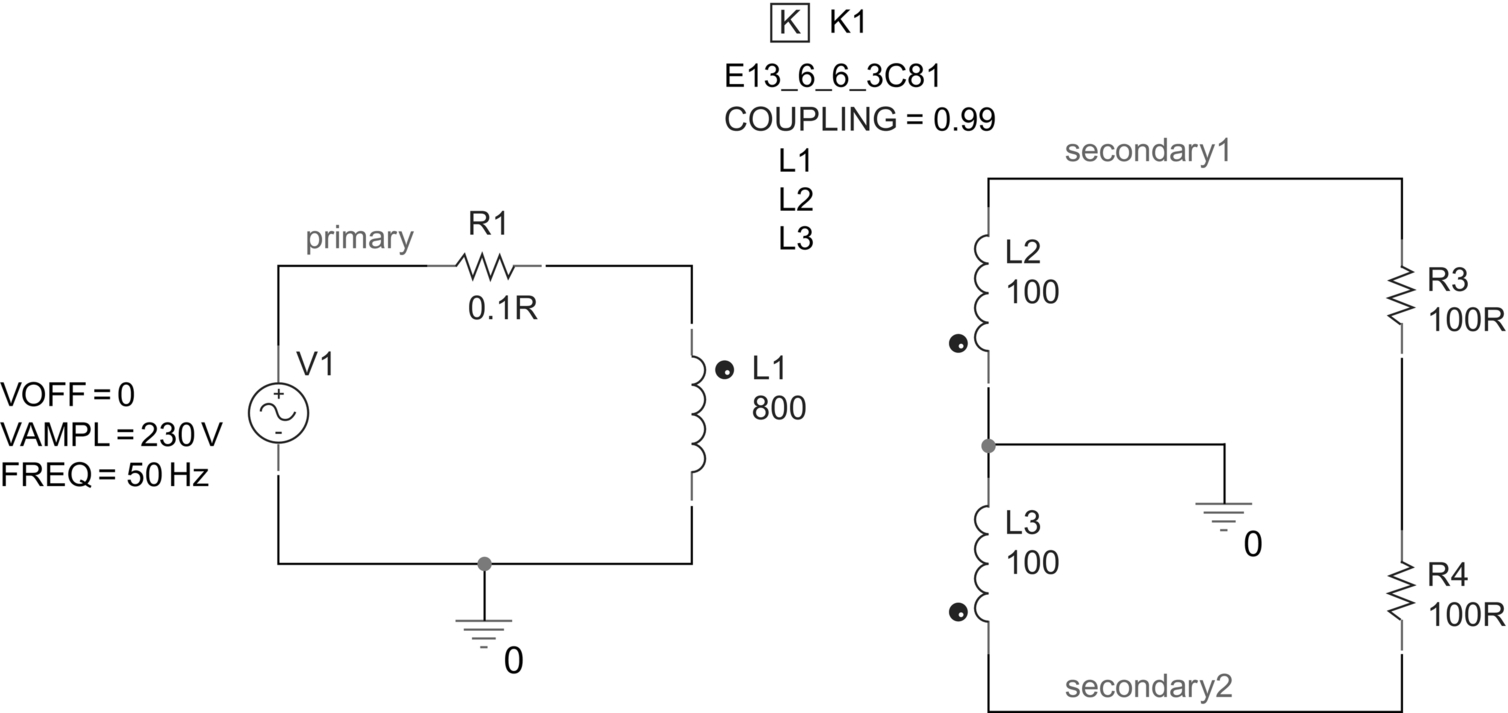
The hysteresis curve for the magnetic cores can be displayed by selecting a K device and rmb > Edit PSpice Model, which will open the PSpice Model Editor. In the Model Editor the text description for the model will be displayed. By selecting View > Extract Model and clicking on Yes to the message window, the characteristic hysteresis curve will be plotted. At the bottom of the Model Editor, is a table of the magnetic core parameters. For each core, there is a gap parameter which can be specified. There is also an entry table whereby you enter B-H curve data and extract your own model parameters. Fig. 9.3 shows the model parameters and hysteresis curve for the E13_6_6_3C81 magnetic core. The Model Editor will be covered in more detail in Chapter 16.

9.3 Predefined Transformers
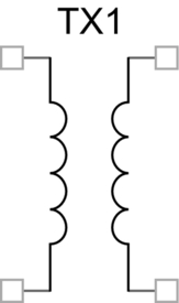
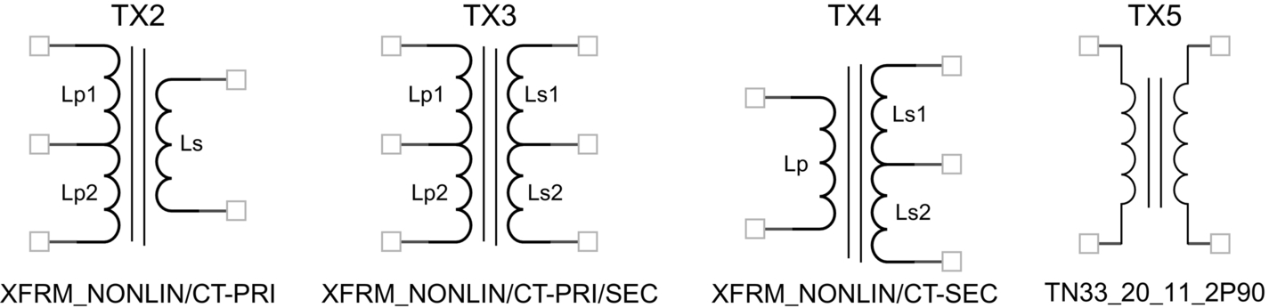
A linear transformer, XFRM_LINEAR (Fig. 9.4), is available in the analog library. Nonlinear transformers, which include center-tapped primary and secondary windings, can be found in the breakout library (Fig. 9.5). These transformers have properties that enable you to enter the inductance, coil resistances and number of turns. Double click on the transformers to access the properties in the Property Editor.
9.4 Exercises
Exercise 1
You will create a step-down transformer circuit with a primary inductance winding inductance of 3.1 H and a winding resistance of 0.2 Ω. The secondary winding has an inductance of 31 mH and a winding resistance of 0.2 Ω. The transformer provides a step-down ratio of 10 and is connected to a 100 Ω load resistance.
1. Create a new project called Linear Transformer and draw the circuit in Fig. 9.6. The inductors, resistors and K_Linear are all from the analog library. V1 is a VSIN source from the source library. Set the coupling coefficient to 0.65.
2. If you have a previous version of OrCAD which does not have the dot convention shown on the inductors, then display pin 1 of the inductors and orientate the inductors accordingly.
3. Double click on the K_Linear device to open the Property Editor and add the inductor reference designators as shown in Fig. 9.7. Highlight L1 and L2, then rmb > Display and select Value Only (Fig. 9.8).

Note
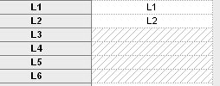
A common misunderstanding is that the coil reference designators must be entered as L1 to L6 in the Property Editor. If you have coils with reference designators L3, L4 and L5 in a circuit, then you enter the designators as shown in Fig. 9.9. It is recommended that you show the reference designators on the schematic for a K core device, especially if you annotate and change the coil numbering.

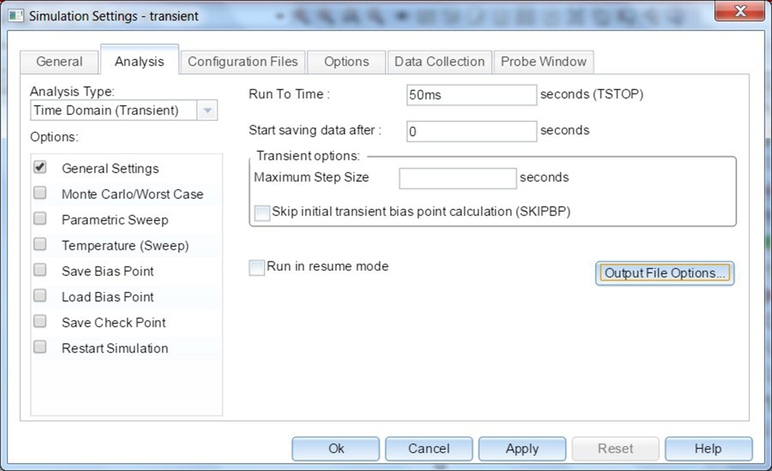
4. Set up a transient simulation profile with a Run to time of 50 ms (Fig. 9.10).
5. Place voltage markers on the primary and secondary nets and run the simulation. You should see the response as shown in Fig. 9.11 with a secondary voltage of 6.4 V.
If you have not placed markers on the circuit then when the PSpice window appears, select Trace > Add Trace and select from the left-hand side under Simulation Output Variables, V(primary) and V(secondary).

6. The relationship between the primary and secondary voltages and the primary and secondary inductances for air cored transformers is given by:

So, if you increased k to 1 you would see a secondary voltage of approximately 10 V. In practice, air cored transformers have a low coupling coefficient.
Exercise 2
You will create a nonlinear, center-tapped transformer circuit.
1. Create a new project called Non Linear Transformer and draw the circuit in Fig. 9.12. Enter the inductor values as the number of turns as shown. The E13_6_6_3C81 core model is found in the magnetic library. Enter a value of 0.99 for the coupling coefficient.

2. As in Exercise 1, double click on the K core device and in the Property Editor, add and display the reference designators L1, L2 and L3.
3. Create a transient simulation profile with a run to time of 50 ms.
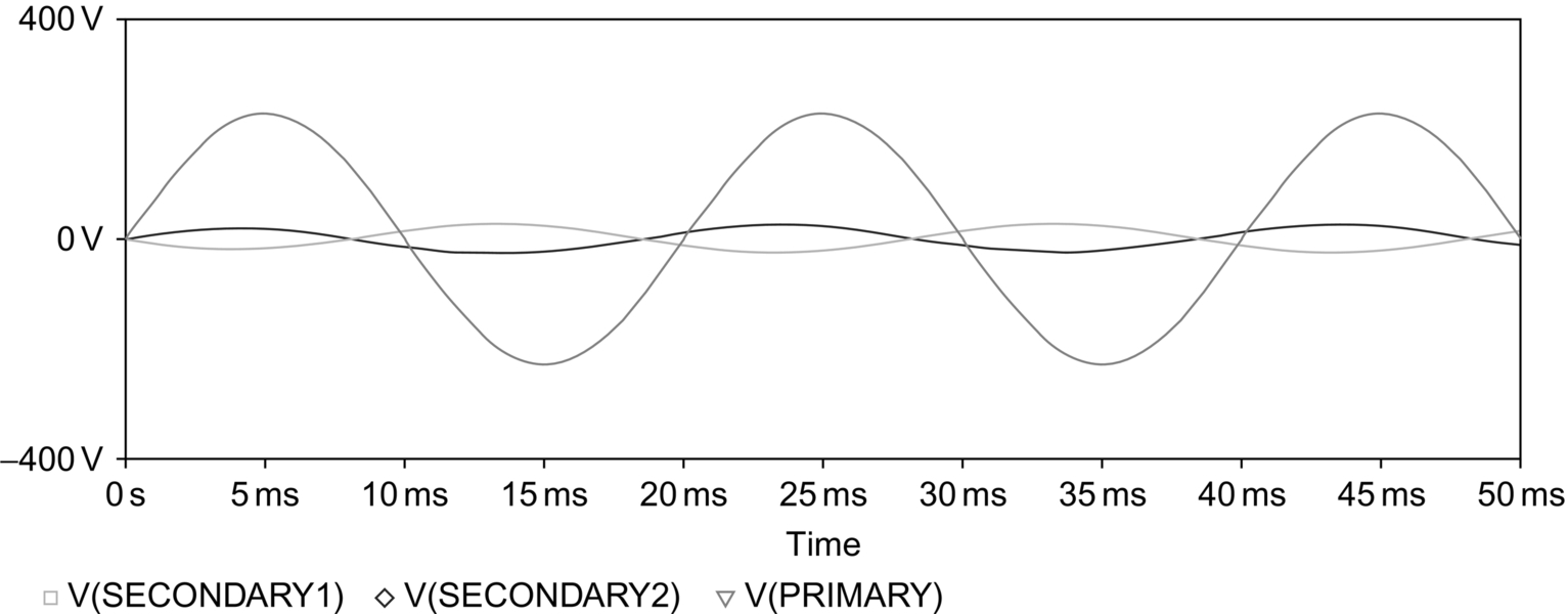
4. Place voltage markers on the nets, primary, secondary1 and secondary2 and run the simulation.
5. Fig. 9.13 shows the voltage waveforms for the nonlinear transformer. You should see 25.1 V on each secondary winding.
6. Investigate the other transformers in the analog and breakout libraries.