Search in book...
Toggle Font Controls
Create new playlist

Name your new playlist

Playlist description (optional)
Sign In

Email address

Password

Forgot Password?

or

Continue with Facebook

Continue with Google
Sign Up

Full Name

Email address

Confirm Email Address

Password

or

Continue with Facebook

Continue with Google

Chapter 24

Sensitivity Analysis

Abstract

Sensitivity Analysis is used to identify components that are most sensitive to circuit performance. The sensitivity of a circuit is defined as the ratio of the change in an output measurement of a circuit, to a change in a circuit parameter value that has a defined tolerance. Typically you would analyze the gain of a circuit, the frequency response, noise figure, etc. for a change in component values up to their tolerance limits. This will enable you to tighten up on tolerances for critical components and conversely to relax tolerances for noncritical components.

Keywords

Sensitivity; Tolerance; Absolute; Relative; Worst case

Introduction

Sensitivity analysis is run in conjunction with a transient, AC, or DC sweeps and uses measurement expressions on the resultant output waveforms. An initial nominal simulation run is performed using nominal component values with all tolerances set to zero. Individual component tolerances are then set in turn to 40% of their maximum positive limit while keeping all other components at their nominal values in order to determine the effect each component has on circuit performance. A Worst Case analysis is then run to determine the maximum and minimum measured values by setting component values to their respective tolerance limits. The Worst Case analysis does not take into account the interdependence of the component parameters. Worst Case analysis assumes a linear tolerance relationship between the 40% and 100% values and also for the 1% interpolated value for the relative sensitivity calculation.

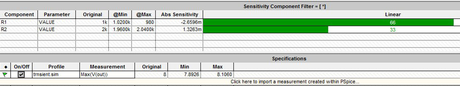
Fig. 24.1 shows the result of the sensitivity analysis that lists the components in order that have the greatest effect or deviation from the nominal measured value. It can be seen that in the top window (Sensitivity Component Filter), R3 and R4 are the most sensitive components and R1 has the least significant effect on circuit performance. The Worst Case results shown in the Specifications window indicate the maximum and minimum measured values from the original values for V(out) and I(R5). By default, the sensitivity analysis values are calculated in the linear domain but can also be calculated in the logarithmic domain. However, the logarithmic values are not displayed in the bar graphs.

Note

Sensitivity analysis in Advanced Analysis is different to sensitivity analysis in PSpice A/D in that tolerance properties and parameters are assigned to components rather than using the simulation setting, RELTOL to set up the tolerance values.

24.1 Absolute and Relative Analysis

There are two types of sensitivity analysis, absolute and relative. Absolute sensitivity is related to a unit change in a parameter value, i.e., a 1 ohm change in resistor value, whereas relative sensitivity is related to a unit percentage change in parameter value, i.e., a 1% change in resistor value. Advanced Analysis calculates both absolute and relative sensitivities but because of typically small capacitor and inductor values being used in circuits, a unit change of 1 Farad for capacitors and 1 Henry for inductors are not realistic, hence the results of relative sensitivity are typically used for capacitors and inductors. The results of the sensitivity and Worst Case analysis are written to the log file, View > Log File > Sensitivity.

The sensitivity calculations are based on the following equations:

Absolute Sensitivity

$S_{A} = \frac{M_{S} - M_{N}}{{P_{N}}^{*} {S_{V}}^{*} Tol}$

si1_e (24.1)

where M_S, measurement value from the sensitivity run for specified parameter; M_N, measurement value from the nominal run; P_N, nominal value of specified parameter; S_V, sensitivity variation (default 40%); and Tol, relative tolerance of the specified parameter.

Relative Sensitivity

$S_{R} = \frac{M_{S} - M_{N}}{{S_{V}}^{*} Tol} \times 1 %$

si2_e (24.2)

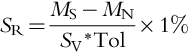
where M_S, measurement value from the sensitivity run for specified parameter; M_N, easurement value from the nominal run; S_V, sensitivity variation (default 40%); Tol, relative tolerance of the specified parameter.

Eqs. (24.1), (24.2) are related by

$Relative sensitivity = absolute sensitivity \times Pn$

(24.3)

24.2 Example

For example, for the simple voltage divider resistor network in Fig. 24.2, sensitivity analysis will determine how the voltage at node out is affected by the resistor tolerances by using the Max measurement on the output voltage.

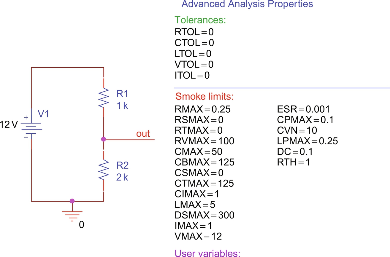
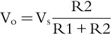
The two resistors in Fig. 24.2 both have a tolerance of 2%. The output voltage is given by

$V_{o} = V_{s} \frac{R 2}{R 1 + R 2}$

si4_e

R1 = 1000 Ω ± 2% or R1 = 1000 Ω ± 20 Ω

R2 = 2000 Ω ± 2% or R2 = 2000 Ω ± 40 Ω

Using nominal values:

$V_{o} = 12 \frac{2000}{1000 + 2000} = 8 V$

si5_e

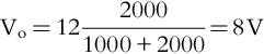
Running a transient analysis and setting up a Max measurement (Trace > Evaluate Measurement), a nominal voltage of 8 V will be measured.

Advanced Analysis will initially run a nominal analysis using nominal values for the resistors and return a measured value for M_N of 8 V. The results of the simulation can be found in the log file, View > Log File > Sensitivity.

For absolute sensitivity analysis:

Advanced Analysis will then set the value of R1 to 40% of its maximum positive tolerance limit that equates to 0.4 × 2 = 0.8%. So, R1 assumes a value of 0.8% × 1000 = 1008 Ω for the next simulation run. The output voltage from the voltage divider is now calculated as M_S = 7.97872340425532 V.

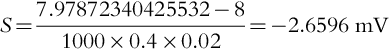
$S = \frac{7.97872340425532 - 8}{1000 \times 0.4 \times 0.02} = - 2.6596 mV$

si6_e

The negative value for the sensitivity ties in with the fact that as R1 increases, Vout decreases from the nominal value.

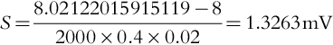
Similarly for R2, the value will be set to R2 to 40% of its maximum positive tolerance limit that equates to 0.4 × 2 = 0.8%. So R2 assumes a value of 0.8% × 2000 = 2016 Ω for the next simulation run. The output voltage from the voltage divider is now calculated as M_S = 8.02122015915119 V.

$S = \frac{8.02122015915119 - 8}{2000 \times 0.4 \times 0.02} = 1.3263 mV$

si7_e

For relative sensitivity:

The relative sensitivities for a 1% change in parameter tolerance value are calculated using Eq. (24.3):

$Relative sensitivity = absolute sensitivity \times Pn \times 1 %$

Therefore the relative sensitivities for the voltage divider circuit are given by

$Relative sensitivity = - 2.6595745 \times 10^{- 3} \times 1000 \times 0.01 = - 26.5957 mV$

$Relative sensitivity = 1.3262599 \times 10^{- 3} \times 2000 \times 0.01 = 26.5252 mV$

24.3 Assigning Component and Parameter Tolerances

The passive components in the analog library include resistors, capacitors, and inductors that have a tolerance property that allow standard symmetric tolerance values to be added to the component, i.e., a 10 kΩ ± 2%. For asymmetric tolerances, as in the case of some electrolytic capacitors, the passive components in the advanals > pspice_elem library allow POSTOL and NEGTOL tolerances to be defined, i.e., 10000 μ + 20%, − 30%. If only POSTOL is defined, then by default, NEGTOL assumes the value of POSTOL.

The tolerance values can be set locally on individual passive components using the Property Editor or they can be set globally to apply a number of components in one go using either the Variables part from the advanals > pspice_elem library or using the Assign Tolerance window that is available in the later 17.2 software versions.

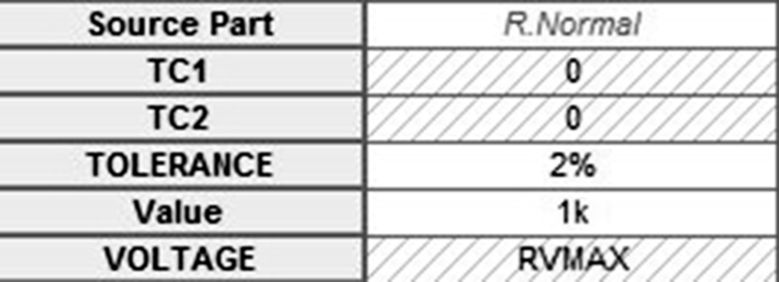
Fig. 24.3 shows the TOLERANCE property for a resistor set to 2% in the Property Editor. You do not have to enter the % sign in the Property editor but is useful if you want to display the component tolerance value with a % sign on the circuit diagram.

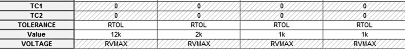
Alternatively, the component tolerance can be set globally to a number of components in one go using the Variables part as shown in Fig. 24.4. In the Property Editor, the value of the TOLERANCE property is set to RTOL as shown in Fig. 24.5 such that the four resistors with the RTOL value will be assigned a tolerance of 2%.

Fig. 24.5 Globally assigning component tolerance values using RTOL from the variables part.

Note

Global tolerance values can be overridden by setting a local tolerance value on an individual passive component.

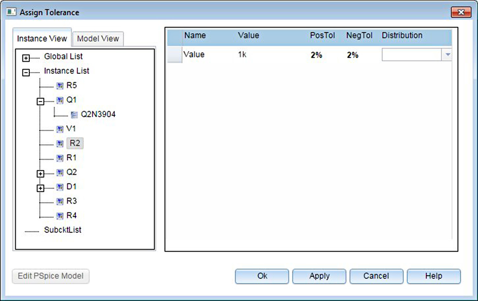
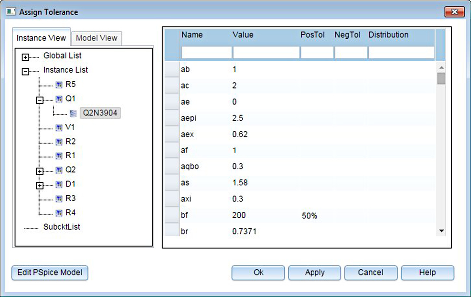
From 17.2 onward, the Assign Tolerance window from PSpice > Advanced Analysis > Assign Tolerance can be used to assign component tolerances and distribution for Monte Carlo analysis to passive devices. Individual components can be selected and positive and negative tolerances assigned (Fig. 24.6).

The Assign Tolerance window also displays the PSpice model and subcircuit parameters for active components that can be assigned a tolerance and distribution for the Monte Carlo analysis. From the Assign Tolerance window, you can open the Model Editor. The Assign Tolerance window is then updated to display those model parameters as shown in Fig. 24.7.

Fig. 24.7 2N3904 PSpice model parameters.

Note

For the PSpice Advanced Analysis Lite version, Sensitivity analysis can only be run on a maximum of three components with tolerances and only one measurement specification. The maximum number of runs is limited to 20.

Note

For the following exercises it is assumed that you are familiar with using the Property Editor that was introduced in Chapter 5, familiar on how to set up and run a PSpice Simulation transient analysis in Chapter 7, and are familiar with Measurement Expressions that was introduced in Chapter 12.

24.4 Exercises

Exercise 1

Assigning local Smoke parameter properties for tolerance.

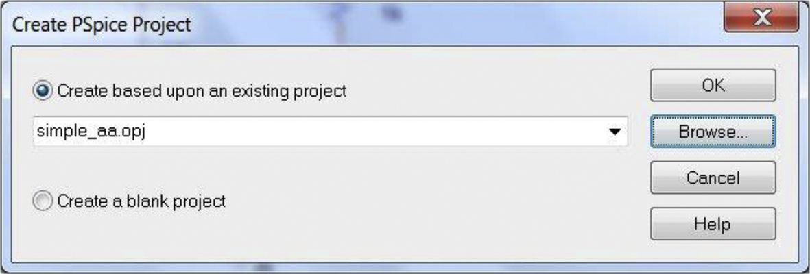
1. Create a new project called for example resistor_network. After you name the project, the project folder the Create PSpice Project window appears. In the pull down menu, select the simple_aa.opj (Fig. 24.9) and click on OK.

Fig. 24.9 Setting up default Advanced Analysis libraries.

Note

In the latest versions of OrCAD, when you first open the schematic page, the Variables part will automatically appear. If you select Empty Project, or you have inadvertently deleted the Variables part, then this can be added from the PSpice > advanals > pspice_elem library.

2. Draw the circuit in Fig. 24.8 using resistors from the analog library.

3. You need to assign a tolerance of 2% to each of the two resistors using the Property Editor. Hold the control key down and highlight both resistors and then double click on one of the resistors or you can rmb > Edit Properties. The properties associated with both resistors will appear in the Property Editor (See Chapter 5).

4. For the TOLERANCE property, enter 2% for each resistor. Highlight the TOLERANCE property so that both resistor values of 2% are highlighted and click on the Display button (or rmb > Display). In the Display Properties window (Fig. 24.10), select Value Only and click on OK. Close the Property Editor. You should see the TOLERANCE property values of 2% displayed on the circuit diagram.

5. Create a Transient analysis. PSpice > New Simulation Profile. Leave the Run to Time to the default value of 1000 ns. Place a voltage marker on the node “out.”

6. PSpice will run and display the 8 V output in the Probe window.

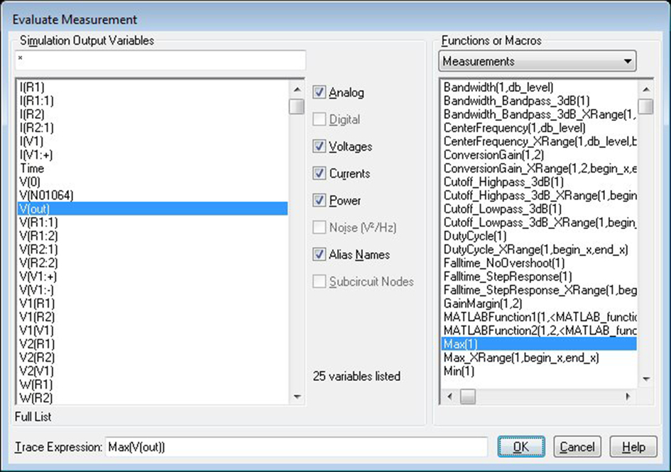
7. You need to add a measurement expression (Chapter 12) to the output of the circuit. Select Trace > Evaluate Measurement that will open up the Evaluate Measurement window. Select Max(1) from the Functions and Macros list and then select V(out), see Fig. 24.11. Click on OK.

Fig. 24.11 Defining a measurement expression.

8. In Probe you should see the result of the measurement Expression as shown in Fig. 24.12.

9. Go back to Capture and run the Sensitivity analysis, PSpice > Advanced Analysis > Sensitivity.

Note

If a Cadence Product Choices menu opens, then just select PSpice Advanced Analysis.

10. Advanced Analysis will launch showing the Sensitivity analysis window. You need to import a Measurement Expression for the analysis. Under Specifications click on the text, “Click here to import a measurement created within PSpice …” In the Import Measurement(s) window click on the Max[V(out)] measurement and click on OK. Run the sensitivity simulation by clicking on the green Play button.

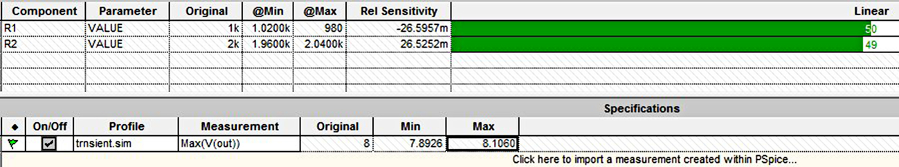
11. Fig. 24.13 shows the results of the Sensitivity analysis showing the absolute sensitivity values for R1 and R2 and the Worst Case results, maximum and minimum for V(out).

12. Open the Log File, View > Log File > Sensitivity, to see a summary of the Sensitivity runs, Fig. 24.14.
Using Eq. (24.1) for Absolute Sensitivity for R1:

$S = \frac{7.97872340425532 - 8}{1000 \times 0.4 \times 0.02} = - 2.6596 mV$

si11_e

Using Eq. (24.1) for Absolute Sensitivity for R2:

$S = \frac{8.02122015915119 - 8}{2000 \times 0.4 \times 0.02} = 1.3263 mV$

si12_e

13. Right mouse button (rmb) anywhere in the top window pane under Sensitivity Component Filter, i.e., under the Linear field and select, Display > Relative Sensitivity (Fig. 24.15).
Using Eq. (24.2) for relative sensitivity for R1:

Fig. 24.15 Sensitivity analysis results.

$S = \frac{7.97872340425532 - 8}{0.4 \times 0.02} \times 0.01 = 26.5957 mV$

si13_e

Using Eq. (24.2) for relative sensitivity for R1:

$S = \frac{8.02122015915119 - 8}{0.4 \times 0.02} \times 0.01 = 26.5252 mV$

si14_e

The results of the Worst Case analysis for maximum and minimum measured values are calculated as:

sensitivity minimum run: R1 + 2%, R2 − 2% Vo = 7.89261744966443 V

sensitivity maximum run: R1 − 2%, R2 + 2% Vo = 8.10596026490066 V

The value in the green bar is calculated as a percentage of the total sensitivity.

The Variables symbol can be used to assign tolerances globally to a number of similar passive components such as the two resistors in Exercise 1. You need to replace the 2% tolerance with the global RTOL tolerance property on the Variables symbol and set RTOL to 2%. If the 2% values are displayed, double click on each 2% tolerance value and replace the text with RTOL. If the percentage values are not displayed, then use the Property Editor to replace the 2% value with RTOL.

With the later software version of 17.2, the Assign Tolerances window can be used to assign tolerances to individual components. PSpice > Advance Analysis > Assign Tolerances.

Exercise 2

Fig. 24.16 shows a series regulator circuit using voltage feedback with an opamp. The circuit is designed to have an output voltage of 9 V ± 5% with a maximum output current of 190 mA. R4 represents the load resistance that can vary by 5%.

1. Create a new PSpice project called, for example, voltage_regulator and select the project template simple_aa.opj as you did in Exercise 1.

2. Open the schematic page. In the latest versions of OrCAD, when you first open the schematic page, the Variables symbol will automatically appear. Delete the Variables part as you will be using the Assign Tolerance window to set component tolerances.

3. Draw the circuit in Fig. 24.16. Make sure you label node “out.” The 2N3904 transistor can be found in the eval.olb or bipolar library, resistors are from the analog library, and the zener diode is from the phil_diode.olb or zetex.olb libraries.

Note

All the PSpice libraries are now shipped with the latest 17.2 Lite DVD. The libraries can also be downloaded for free from the OrCAD website or the local Cadence Channel Partner (CCP) website or you can copy them from someone who has the full software version installed.

4. Open the Assign Tolerance window, PSpice > Advanced Analysis > Assign Tolerance.

5. In the Instance List, select R1 and double click in the PosTol column for R1. Enter a value of 2%. Assign tolerances of 2% for resistors R2, R3 and 5% for R4.

6. Close the Assign Tolerance window. By default NegTol will assume the same value as PosTol. You will see this the next time you open the Assign Tolerances window.

7. Open the Assign Tolerance window.

8. Select Q1 and then Q2N3904. Click on Edit PSpice Model to open the Model Editor as you are going to change the transistor gain.

9. At the bottom of the Model Editor in the Model Text pane, change: Bf = 416.4 to Bf = 200 dev = 50%. This adds a tolerance of 50% to the transistor current gain, see Fig. 24.17.

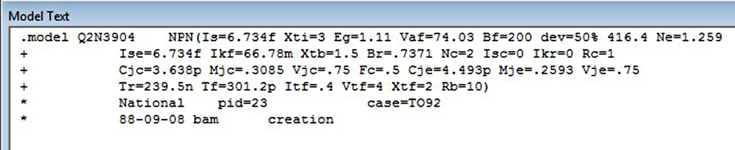
Fig. 24.17 Changing the transistor gain.

10. Close the Model Editor and save the changes.

11. Close the Assign Tolerances window.

Note

When you open the Model Editor, you automatically create a copy of the transistor PSpice model file that has the same name as your project, i.e., power_supply.lib. The original transistor model is not changed.

12. Set up a transient analysis and use the default Run to Time of 1000 ns.

13. Add a PSpice voltage markers to node “out” and a current marker to the bottom pin of resistor R4. This is because current is measured into pin 1 of the resistor that is situated at the bottom end after you have rotated the resistor. If you get a negative result, it just means that the current is flowing out of pin of the resistor. Make sure the current marker is attached to the resistor pin.

14. Run the simulation.

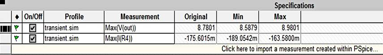
15. As in Exercise 1, you need to add a measurement expression (Chapter 12) to the output of the circuit. Select Trace > Evaluate Measurement that will open up the Evaluate Measurement window. Select Max(1) from the Functions and Macros list and then select V(out) and click on OK. Repeat for load current by Max(1) and then I(R4). You should see the same results as shown in Fig. 24.18.

Fig. 24.18 Viewing the measurement results values.

Note

If you run the simulation again, then you view the previous Measurement results, View > Measurement Result and click in the Evaluate boxes to see the measurement results for the voltage and current outputs.

16. Go back to Capture and run the Sensitivity analysis, PSpice > Advanced Analysis > Sensitivity.

17. Advanced Analysis will launch showing the Sensitivity analysis window. You need to import a Measurement Expression for the analysis. Under Specifications click on the text, “Click here to import a measurement created within PSpice …” In the Import Measurement(s) window select the Max[V(out)] and Max[I(R4)] measurements and click on OK.

18. Run the sensitivity simulation by clicking on the green Play button.

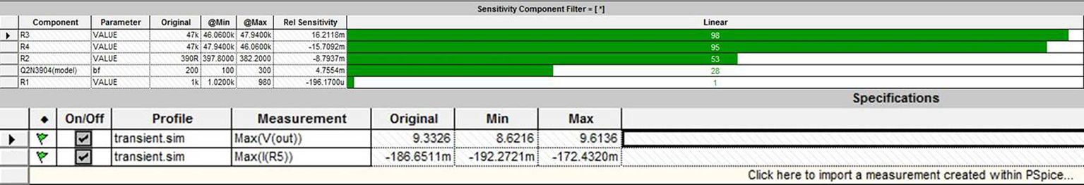
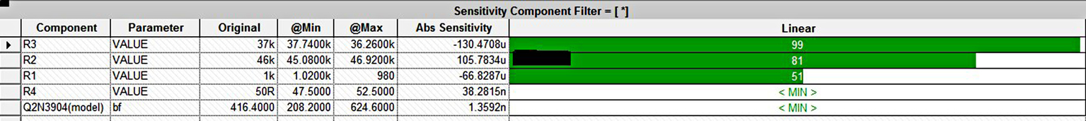
19. Fig. 24.19 shows the results of the Sensitivity analysis showing the absolute sensitivity values for the circuit components and the Worst Case results, maximum and minimum for V(out) and I(R4).

20. In the Sensitivity Component Filter window, right mouse click anywhere and select Display > Relative Sensitivity. Fig. 24.20 shows the results of the Sensitivity analysis showing the relative sensitivity values for the circuit components and the Worst Case results, maximum and minimum for V(out) and I(R4).

Fig. 24.21 shows the results for the Worst Case analysis for V(out) and I(R4).

..................Content has been hidden....................

You can't read the all page of ebook, please click here login for view all page.

Table of Contents for Chapter 24: Sensitivity Analysis

Create new playlist

Sign In

Sign Up

Introduction

24.1 Absolute and Relative Analysis

Absolute Sensitivity

Relative Sensitivity

24.2 Example

24.3 Assigning Component and Parameter Tolerances

24.4 Exercises

Exercise 1

Exercise 2

Table of Contents for
Chapter 24: Sensitivity Analysis