
Monte Carlo Analysis
Abstract
Monte Carlo analysis is essentially a statistical analysis that calculates the response of a circuit when device model parameters are randomly varied between specified tolerance limits according to a specified statistical distribution. Monte Carlo analysis provides statistical data predicting the effect of randomly varying model parameters or component values (variance) within specified tolerance limits. The generated values follow a statistically defined distribution. The circuit analysis (DC, AC, or transient) is repeated a number of specified times with each Monte Carlo run generating a new set of randomly derived component or model parameter values. The greater the number of runs, the greater the chances that every component value within its tolerance range will be used for simulation. Monte Carlo, in effect, predicts the robustness or yield of a circuit by varying component or model parameter values up to their specified tolerance limits. Although the results of a Monte Carlo analysis can be seen as a spread of waveforms in the PSpice waveform viewer (Probe), a Performance Analysis can be used to generate and display histograms for the statistical data together with a summary of the statistical data. This provides a more visual representation of the statistical results of a Monte Carlo analysis. A Monte Carlo analysis is run in conjunction with another analysis, AC, DC, or transient analysis. Tolerances are applied to parts in the schematic via the Property Editor and the required analysis is created in the simulation profile.
Keywords
Monte Carlo; Tolerance; Circuit; Performance analysis; Collating functions
Monte Carlo analysis is essentially a statistical analysis that calculates the response of a circuit when device model parameters are randomly varied between specified tolerance limits according to a specified statistical distribution. For example, all the circuits encountered so far have been simulated using fixed component values. However, discrete real components such as resistors, inductors and capacitors all have a specified tolerance, so that when you select, for example, a 10 kΩ ± 1% resistor, you can expect the actual measured resistor value to be somewhere between 9900 and 10,100 Ω. Other discrete components and semiconductors in a circuit will also have tolerances and so the combined effect of all the component tolerances may result in a significant deviation from the expected circuit response. This is especially the case in filter designs where applied component tolerances may result in a deviation from the required filter response.
What the Monte Carlo analysis does it to provide statistical data predicting the effect of randomly varying model parameters or component values (variance) within specified tolerance limits. The generated values follow a statistically defined distribution. The circuit analysis (DC, AC or transient) is repeated a number of specified times with each Monte Carlo run generating a new set of randomly derived component or model parameter values. The greater the number of runs, the greater the chances that every component value within its tolerance range will be used for simulation. It is not uncommon to perform hundreds or even thousands of Monte Carlo runs in order to cover as many possible component values within their tolerance limits. Monte Carlo, in effect, predicts the robustness or yield of a circuit by varying component or model parameter values up to their specified tolerance limits.
Although the results of a Monte Carlo analysis can be seen as a spread of waveforms in the PSpice waveform viewer (Probe), a Performance Analysis can be used to generate and display histograms for the statistical data together with a summary of the statistical data. This provides a more visual representation of the statistical results of a Monte Carlo analysis.
10.1 Simulation Settings
A Monte Carlo analysis is run in conjunction with another analysis, AC, DC or transient analysis. Tolerances are applied to parts in the schematic via the Property Editor and the required analysis is created in the simulation profile. For the band pass filter in Fig. 10.1, component tolerances have been added to the resistors and capacitors and displayed on the circuit. The circuit response is analyzed by performing an AC sweep from 10 Hz to 100 kHz. Monte Carlo will run an initial analysis with all nominal values being used and then run subsequent analysis using randomly generated component values up to the number of Monte Carlo runs specified.
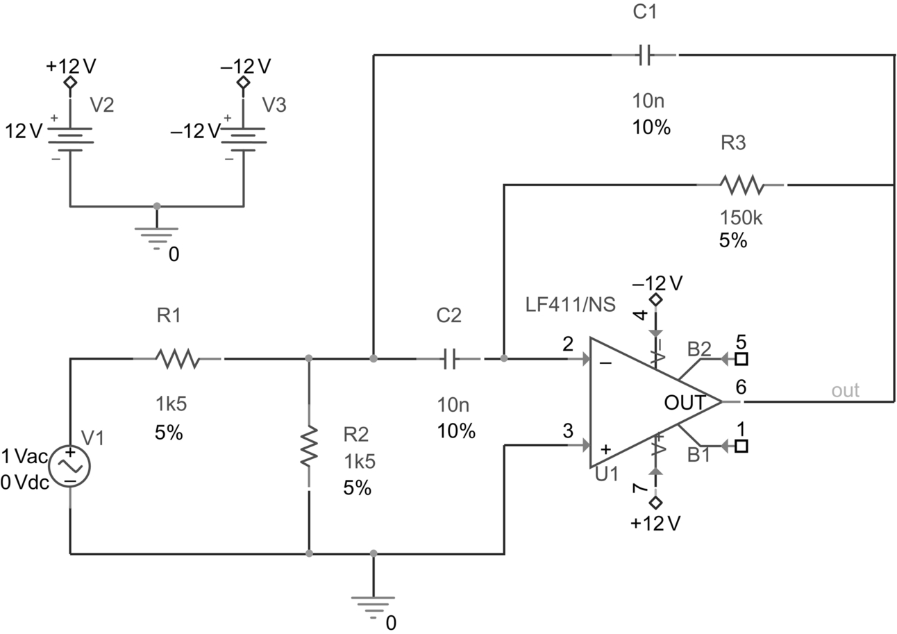
Fig. 10.2 shows the simulation profile for an AC sweep running a Monte Carlo analysis.

10.1.1 Output Variable
You need to specify a node voltage or an independent current or voltage source. In this example, the output variable is V(out).
10.1.2 Number of Runs
This is the number of times the AC, DC or transient analysis is run. The maximum number of waveforms that can be displayed in Probe is 400. However, for printed results, the maximum number of runs has now been increased from 2000 to 10,000. The first run is the nominal run where no tolerances are applied.
10.1.3 Use Distribution
The model parameter deviations from the nominal values up to the tolerance limits are determined by a probability distribution curve. By default, the distribution curve is uniform; that is, each value has an equal chance of being used. The other option is the Gaussian distribution, which is the familiar bell-shaped curve commonly used in manufacturing. Component values are more likely to take on values found near the center of the distribution compared to the outer edges of the tolerance limits.
You can also define your own probability distribution curves using coordinate pairs specifying the deviation and associated probability, where the deviation is in the range − 1 to + 1 and the probability is in the range from 0 to 1. More information can be found in the PSpice A/D Reference Guide in < install dir > docpspcrefpspcref.pdf.
10.1.4 Random Number Seed
As with most random number generators, an initial seed value is required to generate a set of random numbers. This value must be an odd integer number from 1 to 32,767. If no seed number is specified, the default value of 17,533 is used.
10.1.5 Save Data From
This allows you to save data from selected runs. For example, if you just want to see the circuit response from the nominal run, select none. If you want to save all the runs, select All. If you want to select every third run from the nominal run, i.e. the fourth, seventh, tenth, etc., select Every, then enter 3 in the runs box. If you want to save data from the first three runs, select First and then enter 3 in the runs box. If you want to save data from the third, fifth, seventh and tenth run, select Runs (list) and enter 3, 5, 7, 10 in the runs box. Saved runs will be displayed in Probe.
10.1.6 MC Load/Save
PSpice now has history support which allows you to save randomly generated model parameters or component values from a Monte Carlo run in a file, which can be used for subsequent analysis.
10.1.7 More Settings
This option allows you to specify Collating Functions which are applied to the output waveforms returning a single resulting value. For example, the MAX function searches for and returns the maximum value of a waveform. The YMAX function returns the value corresponding to the greatest difference between the nominal run waveform and the current waveform. The RISE and FALL functions search for the first occurrence of a waveform crossing above or below a set threshold value. For each function, you can specify the range over which you want to apply these functions. Fig. 10.3 shows the available collating functions.

The collating functions are summarized as:
YMAX: Find the greatest difference from the nominal run
MAX: Find the maximum value
MIN: Find the minimum value
RISE_EDGE: Find the first rising threshold crossing
FALL_EDGE: Find the first falling threshold crossing
10.2 Adding Tolerance Values
Tolerances can now be added to the discrete R, L and C parts in the Property Editor as these parts now include a tolerance property. You must make sure that you include the % symbol when entering the tolerance value i.e. 10%.
In previous OrCAD versions the only way to add tolerances to discrete parts was to use generic Breakout parts, which allowed you to edit the PSpice model. For example, to add a tolerance to a resistor, you had to use an Rbreak part from the breakout library, edit the model (rmb > Edit PSpice Model) and add tolerance statements to the PSpice model. The default model definition for an Rbreak is given by:
where Rbreak is the model name that can be changed and appears on the schematic, RES is the PSpice model type and R is a resistance multiplier. There are two types of tolerance you can add, dev and lot, as shown below:
.model Rmc1 RES R = 1 lot = 2% dev = 5%
Here, the model name has been changed to Rmc1 and two tolerance types have been added to the model statement. The dev tolerance causes the tolerance values of devices that share the same model name (Rmc1 in this example) to vary independently from each other, while the lot tolerance will cause the tolerance values of devices, with the same model name, to track together.
Dev is the same as applying a standard 5% tolerance to all the resistors, where each resistor with the same model name will be assigned its own random resistance value independent from all the other resistors with the same model name.
Lot is where all the resistors with the same model name will be treated as one group and will track together by as much as ± 2%. This was mainly used in integrated circuit (IC) design where a change in temperature was equally applied to groups of components. The combined total tolerance for Rmc1 can therefore be as much as ± 7%.
One example in which you would use both lot and dev is for a single in-line (SIL) or dual in-line (DIL) resistor pack; each resistor will have a dev tolerance defined, and therefore each randomly generated resistance value will have a different value from the others. If there is a rise in temperature, the lot tolerance will ensure that all resistance values increase together by the same percentage.
As mentioned above, only discrete parts have an attached tolerance property which can be edited in the Property Editor. If you want to add for example a specified manufacturer's tolerance to the Bf of a transistor to see its effect on a circuit's performance, you will have to edit the transistor model and add, for example, the dev tolerance to the Bf model parameter as:
.model Q2N3906 PNP (Is = 1.41f Xti = 3 Eg = 1.11 Vaf = 18.7
Bf = 180.7 dev = 50% Ne = 1.5 Ise = 0
In this example, a dev tolerance of 50% with a default uniform distribution has been added to the Bf of the transistor. However, the distribution for the Bf is more likely to be Gaussian, so you would add dev/gauss = 12.5% as PSpice limits a Gaussian distribution to ± 4σ:
.model Q2N3906 PNP (Is = 1.41f Xti = 3 Eg = 1.11 Vaf = 18.7
Bf = 180.7 dev/gauss = 12.5% Ne = 1.5 Ise = 0
10.3 Exercises
Exercise 1
Fig. 10.4 shows a Sallen and Key 1500 Hz band pass filter circuit. Tolerances will be added to the resistors and capacitors and a Monte Carlo analysis will be performed to predict the statistical variation of the band pass frequency.

1. Draw the circuit in Fig. 10.4. If you are using the demo CD, use the ua741 opamps, which can be found in the eval library; otherwise, the LF411 opamp can be found in the opamp library. Performing a Part Search will result in the LF411 opamp being sourced from different manufacturers. It does not matter which one you use. V1 is a VAC source from the source library, used for an AC analysis, and the power symbols are VCC_CIRCLE symbols from Place > Power, renamed + 12 V and − 12 V, respectively.
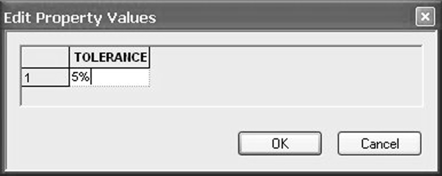
2. You need to add a 5% tolerance to all the resistors. Hold down the control key and select the resistors R1, R2 and R3, then rmb > Edit Properties. In the Property Editor highlight the entire Tolerance Row (or column) as shown in Fig. 10.5 and rmb > Edit. In the Edit Property Values box (Fig. 10.6), type in 5% and click on OK.
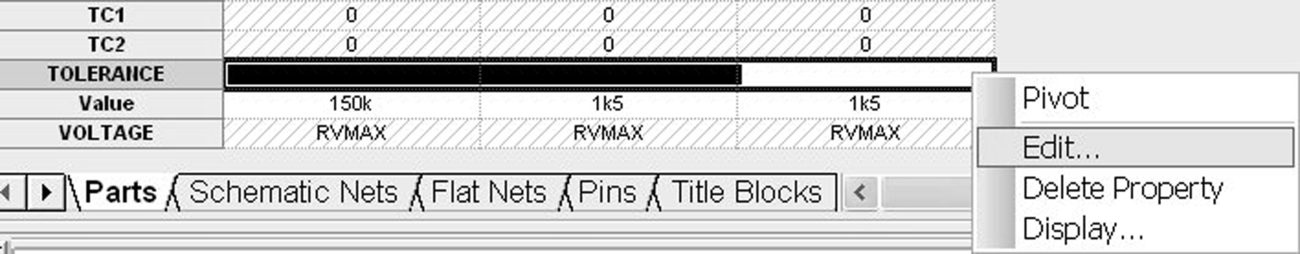
3. To display the component tolerances on the schematic, select the entire TOLERANCE row as in Fig. 10.5, rmb > Display and in Display Properties (Fig. 10.7), select Value Only and click on OK.

4. Repeat Step 2 by assigning a 10% tolerance to capacitors C1 and C2.
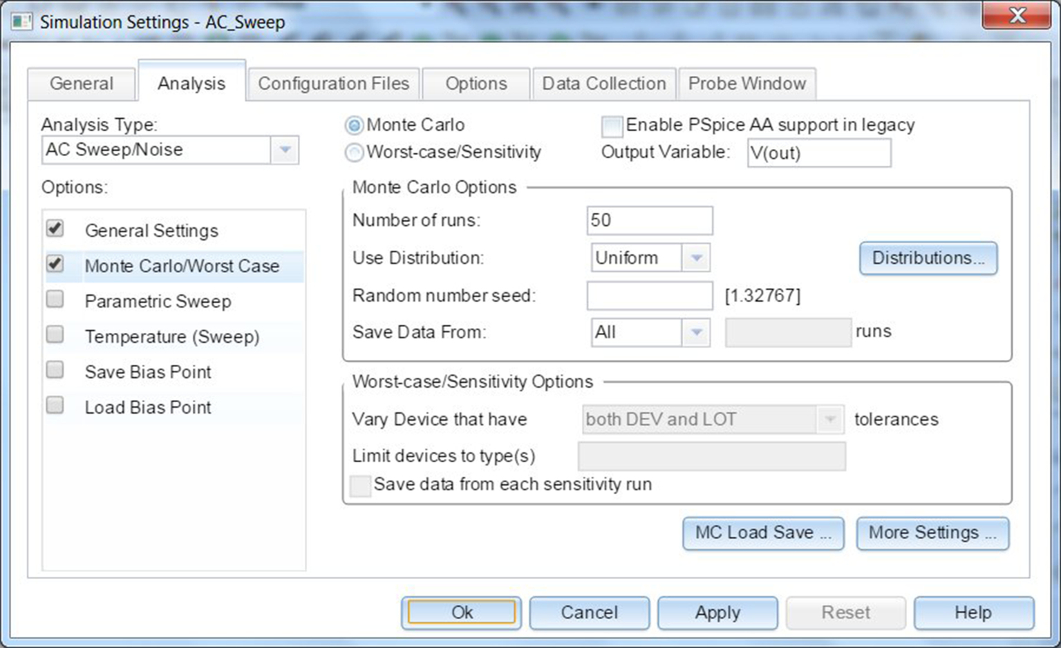
5. Create a PSpice simulation profile called AC Sweep for an AC logarithmic sweep from 100 to 10 kHz with 50 points per decade (Fig. 10.8). Select Monte Carlo/Worst Case in the Options box.
The output variable is V(out) and the number of runs is 50. The distribution used will be uniform and you will use the default random seed setting by leaving the Random number seed box empty. Your Monte Carlo simulation settings should be as shown in Fig. 10.9.

6. Place a dB voltage marker on node out (PSpice > Markers > Advanced > dB Magnitude of Voltage) and run the simulation.
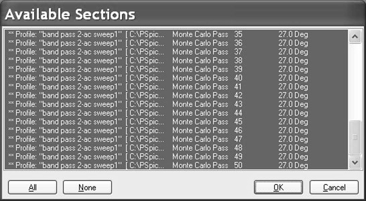
7. When PSpice launches, a list of available runs is shown (Fig. 10.10). Select All and click on OK.
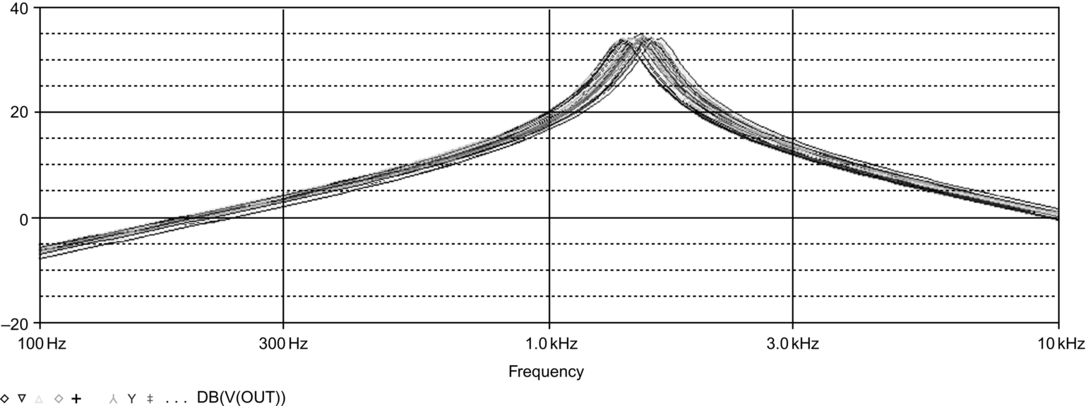
8. Fig. 10.11 shows the band pass filter response showing a spread in the center frequency. Open the output file, View > Output File{ XE “Output File” } and scroll down to see the results for each Monte Carlo run. At the bottom of the file, you will see a summary of the statistical results and the deviation from the nominal for each run.
However, to get a better picture of the spread of the center frequency, you can use a Performance Analysis to display histograms representing the statistically generated data. Performance analysis will be covered in more detail in Chapter 12, but for now, the steps required for a performance analysis for the bandpass filter are introduced in Exercise 2.
Exercise 2
1. In Probe, from the top toolbar, select Trace > Performance Analysis. At the bottom of the Performance Analysis window, click on Wizard, then in the next window click on Next. You will be presented with a list of measurements as shown in Fig. 10.12.
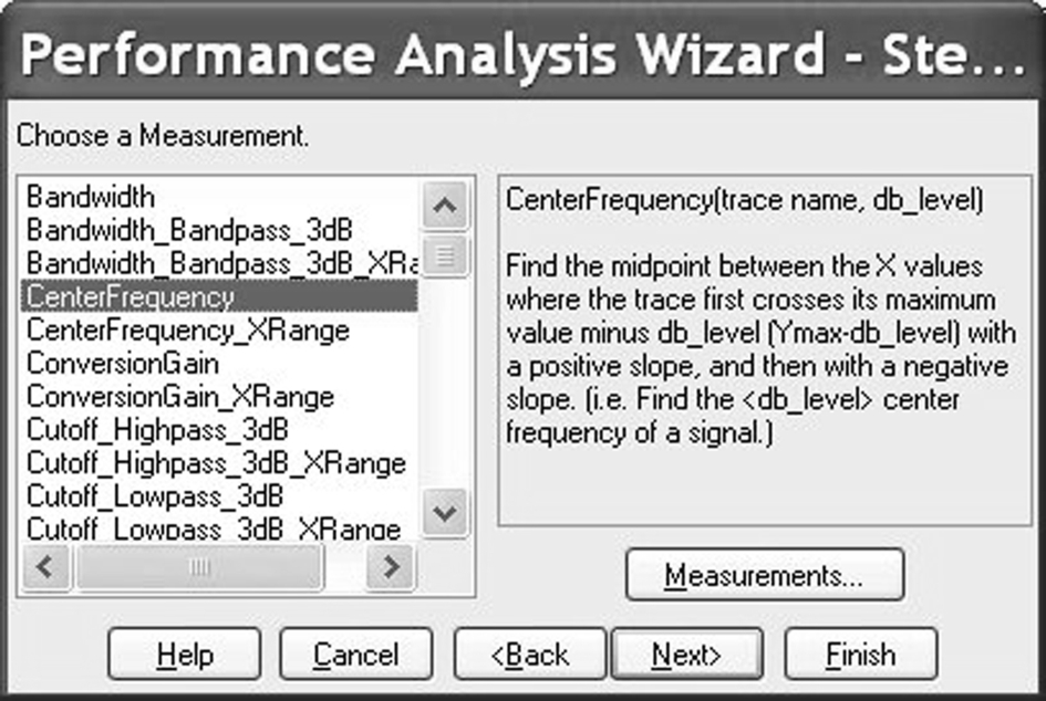
2. Select the CenterFrequency measurement and click on Next.
3. In the Measurement Expression window (Fig. 10.13), enter the name of the trace to search as V(out). Alternatively, you can click on the Name of trace to search icon  and search for the trace name, V(out).
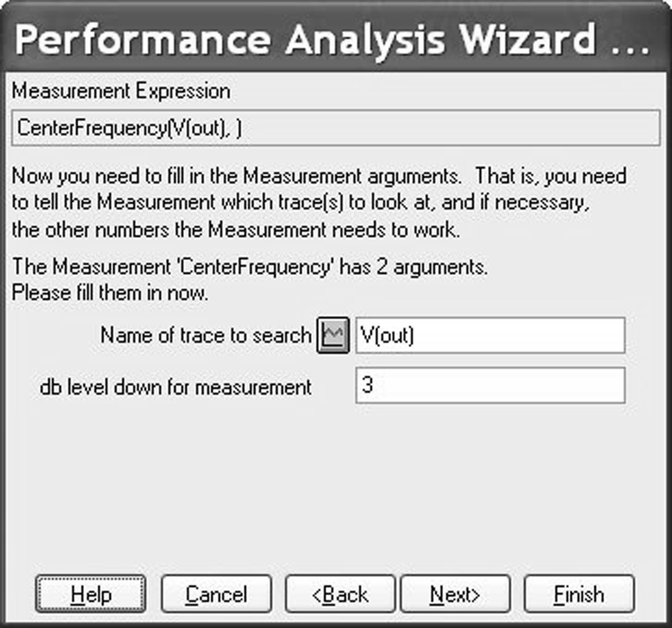
Enter a value of 3 for the db level down for measurement as shown. The center frequency of the filter will be measured 3 dB down either side of the maximum value for the Monte Carlo nominal run (no component tolerances applied). Click on Next in the Performance Analysis Wizard.
4. The nominal trace waveform of the band pass circuit will be displayed (Fig. 10.14). This is the simulation response using the component nominal values. The trace shows two points where the measurements from the waveform will be taken. In this case, the center frequency is defined at 3 dB down from the maximum value. This is shown so that you can confirm whether you are seeing the correct circuit response and that the measurements are taken at the correct points on the waveform.
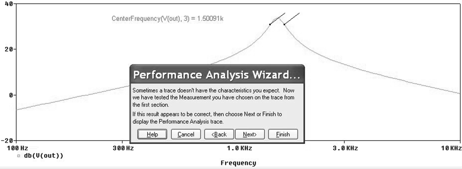
5. Click on Next in the Performance Analysis Wizard.
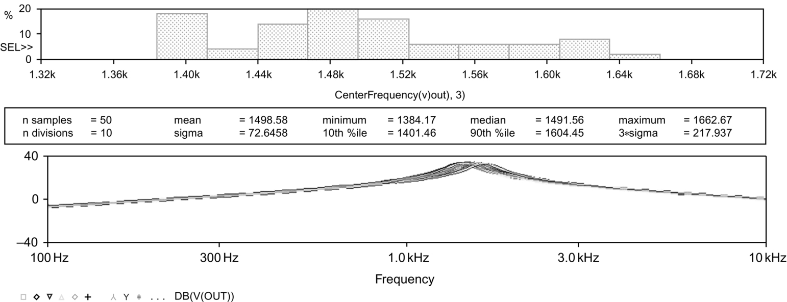
6. Histograms will now be displayed (Fig. 10.15) representing the generated statistical data together with a summary of statistical data.
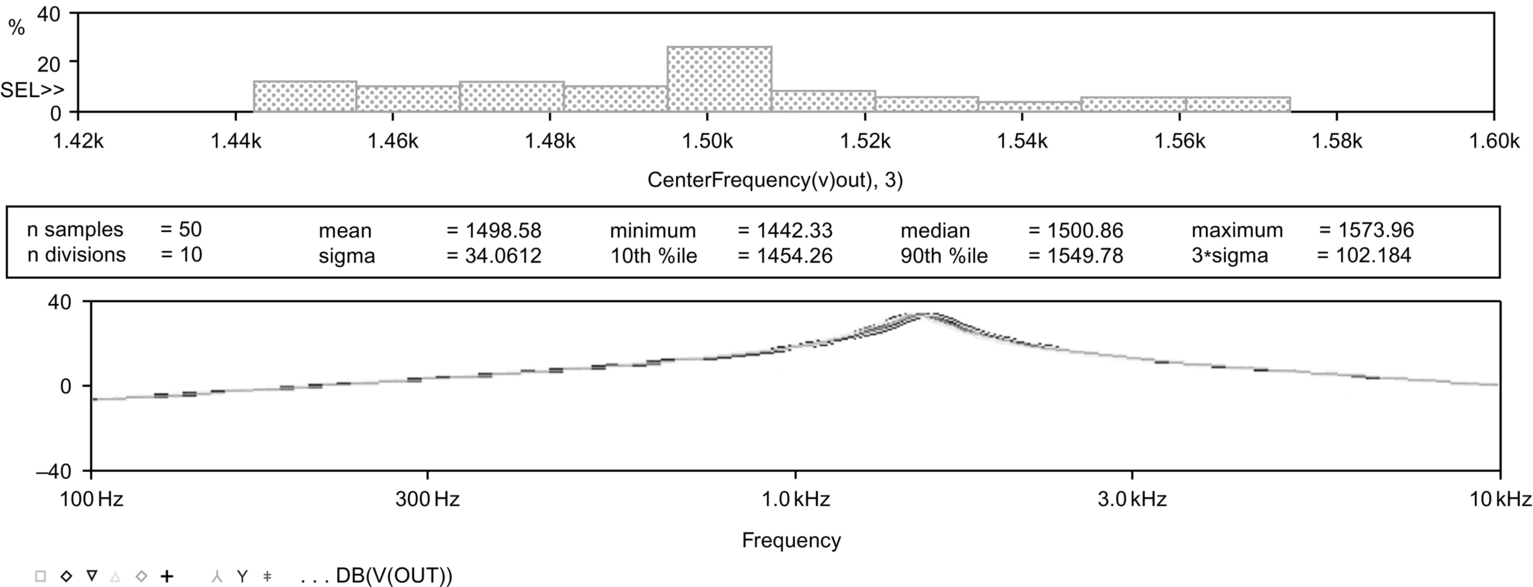
7. Change the resistor tolerances to 1% and the capacitor tolerances to 5% and re-run the simulation. Run a performance analysis as before using the center frequency measurement as above. The results are shown in Fig. 10.16.
8. Run another Performance analysis but this time, use the bandwidth measurement.
Filter Specifications
The gain of the filter is given by:

or in dB:
The band pass center frequency is given by:
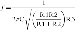
where C1 = C2 = C

The − 3 dB bandwidth is given by:
