Temperature Analysis
Abstract
A change in temperature can affect the performance and characteristics of a circuit. The components most affected by a change in temperature include semiconductors, resistors, capacitors, and inductors. All of these components have an inbuilt temperature dependence model parameter such that performing a temperature sweep will change component and subsequent circuit behavior. The temperature coefficients specified for resistors are given in parts per million per degree Celsius (ppm/°C). In previous versions of OrCAD, the temperature coefficients were not readily available on the Capture parts therefore to add TC1 and TC2. Breakout parts as used for Monte Carlo analysis are used, where the temperature coefficients are added to the PSpice model definition. An AC, DC, or transient analysis is normally run using the default nominal temperature (TNOM) of 27°C, which is set in the simulation profile under the Options tab. TNOM is the default nominal temperature and is also the temperature at which model parameters were measured. If users want to run a transient analysis at a different temperature then they need to specify the simulation temperature by selecting Temperature (Sweep) in the simulation profile and then entering either a single simulation temperature or a list of temperatures values.
Keywords
Coefficient; Temperature; Resistor; Circuit; Simulation; PSpice
A change in temperature can affect the performance and characteristics of a circuit. The components most affected by a change in temperature include semiconductors, resistors, capacitors and inductors. All of these components have an inbuilt temperature dependence model parameter such that performing a temperature sweep will change component and subsequent circuit behavior.
15.1 Temperature Coefficients
For a resistor, the change in its nominal value due to a change in temperature is defined as:
where
TC1—linear temperature coefficient (ppm/°C)
TC2—quadratic temperature coefficient (ppm/°C −2)
T—simulation temperature (°C)
Tnom—nominal temperature (°C), set by default to 27°C
There is a TCE—exponential coefficient which if specified gives the resistor value as:
Manufacturers normally specify the linear coefficient TC1 for resistors.
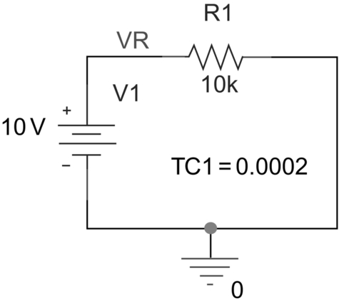
The temperature coefficients specified for resistors are given in parts per million per degree Celsius (ppm/°C). So for a 10 kΩ resistor with a linear temperature coefficient of + 200 ppm/°C, TC1 = 0.0002 and with no TC2 specified, a 20°C rise in temperature will give:
Therefore, for a 20°C rise in temperature, R = 10,040 Ω.
Similarly, for inductors and capacitors the component values are given by:
There is no TCE exponential coefficient for the inductors and capacitors.
In previous versions of OrCAD, the temperature coefficients were not readily available on the Capture parts therefore to add TC1 and TC2. Breakout parts as used for Monte Carlo analysis are used where the temperature coefficients are added to the PSpice model definition.
For example, to add a linear temperature coefficient, TC1 = 0.02 (ppm/°C), place an Rbreak resistor from the Breakout library, rmb > Edit PSpice Model and edit the PSpice model from:
to
.model Rtemp RES R = 1 TC1 = 0.02
15.2 Running a Temperature Analysis
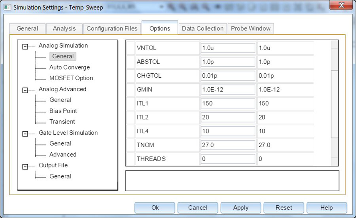
An AC, DC or transient analysis is normally run using the default nominal temperature (TNOM) of 27°C, which is set in the simulation profile under the Options tab (Fig. 15.1). TNOM is the default nominal temperature and is also the temperature at which model parameters were measured.
If you want to run a transient analysis at a different temperature then you need to specify the simulation temperature by selecting Temperature (Sweep) in the simulation profile and then enter either a single simulation temperature or a list of temperatures values as shown in Fig. 15.2.

In the example above, three transient analyses will be run at the specified temperatures of 27°C, 55°C, and 125°C and plotted, one for each temperature, on one graph in Probe, the PSpice waveform viewer.
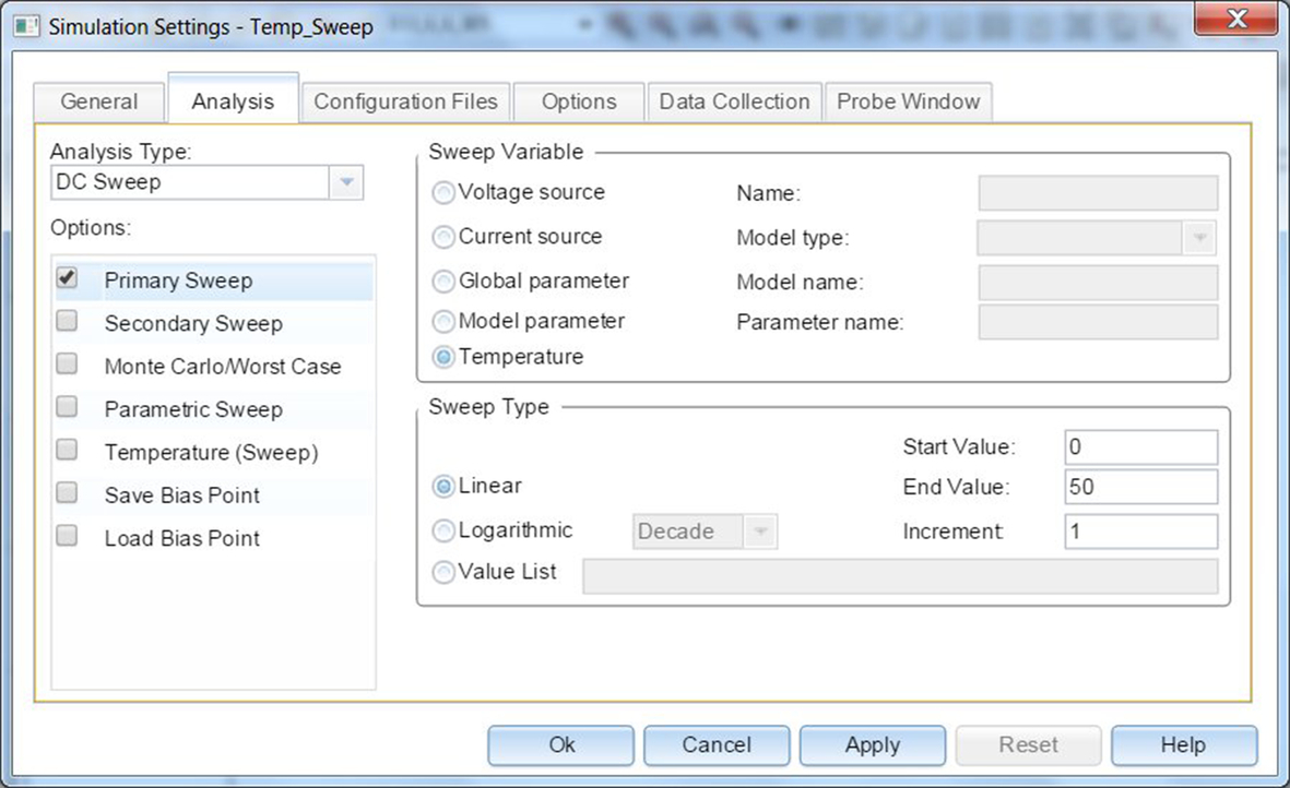
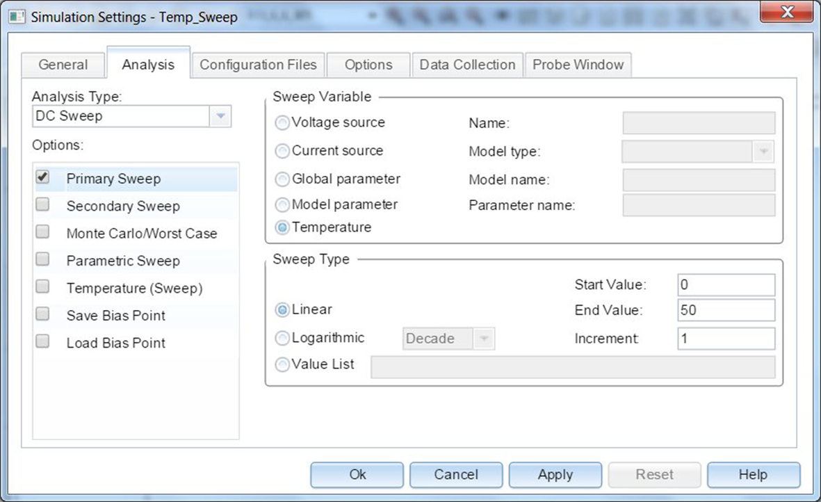
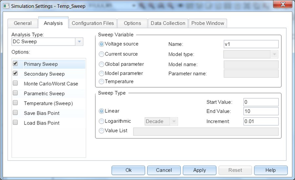
If you want to use temperature as a swept variable, i.e. for temperature to appear on the x-axis, you run a DC sweep and then select temperature as the sweep variable, as shown in Fig. 15.3. The temperature will be swept from 0°C to 50°C in 1°C increments. The change in temperature is represented by T − Tnom.
15.3 Exercises
Exercise 1
The specification for a 10 kΩ resistor is given as 200 ppm/°C. Therefore, TC1 = 0.0002.
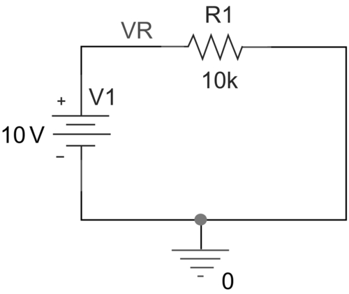
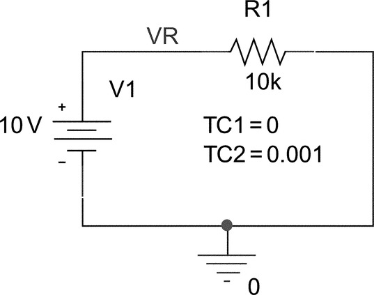
1. Draw the circuit shown in Fig. 15.4 and double click on the resistor to open the Property Editor. Enter a linear coefficient value of 0.0002 in TC1 and Display both the property Name and Value of TC1 as shown in Fig. 15.5. Make sure you name the node as VR, (Place > Net Alias).
2. Set up a DC linear temperature sweep from 0°C to + 50°C in steps of 1°C as shown in Fig. 15.6.
3. Run the simulation.
4. In order to plot resistance, you need to plot the ratio of the voltage across R1 divided by the current flowing through R1. In Probe, select Trace > Add  or
or ![]() .
.
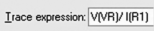
5. At the bottom of the Add Traces window, there is an expression field in which you will define the resistance ratio. Select the V(VR) trace from the list of Simulation Output Variables; then, in the right-hand side Functions or Macros, select the divider symbol “/” and then select I(R1) from the Simulation Output Variables. You should see the expression as in Fig. 15.7.
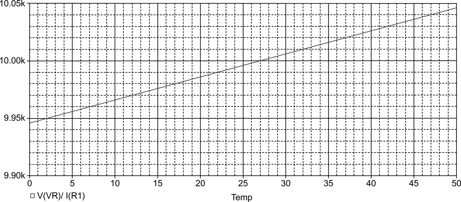
Note that you can also type in the expression rather than select variables or functions. Probe will then display the expected increase in resistance with temperature (Fig. 15.8).
Turn the cursor on and verify that the value of the resistor is 10 kΩ at 27°C and 10,040 Ω at 47°C, which represents a rise in temperature of 20°C.
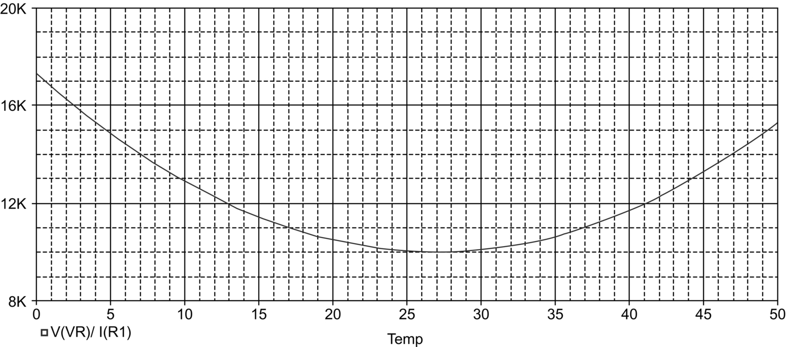
6. Reset TC1 to 0 and add and display the quadratic temperature coefficient, TC2 with a value of 0.001 (Fig. 15.9) and resimulate; but this time, rather than add in the trace expression, you can call up and restore the last display automatically.
7. In Probe, select Window > Display Control > Last Session > Restore. You should see the quadratic response as shown in Fig. 15.10.
Exercise 2
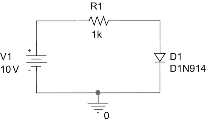
1. Draw the circuit shown in Fig. 15.11. The D1N914 diode can be found in either the diode or eval library.
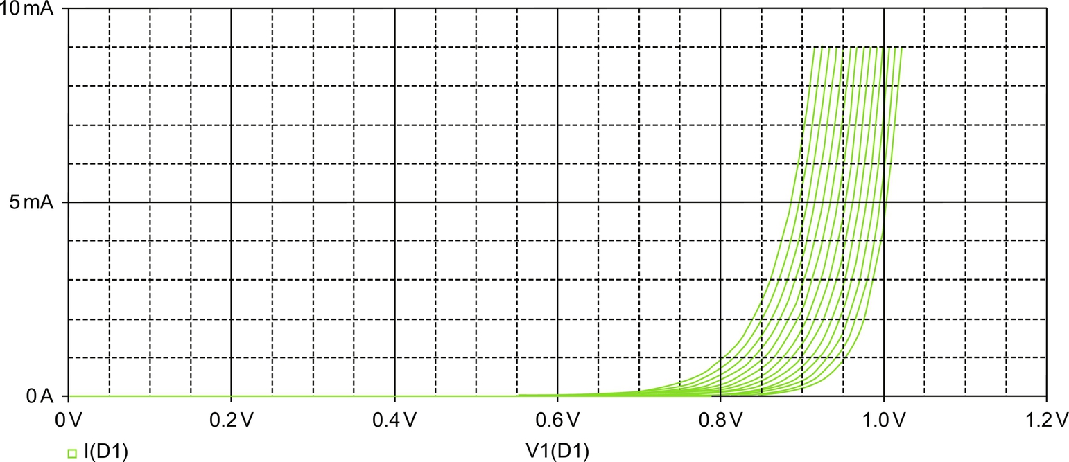
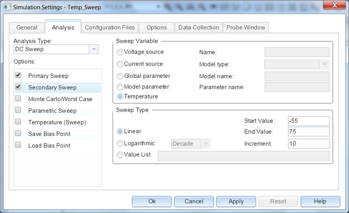
2. Set up a nested DC sweep. For the primary sweep, sweep V1 from 0 to + 10 V in steps of 0.01 V (Fig. 15.12). For the secondary sweep, sweep the temperature from − 55°C to + 75°C in steps of 10°C (Fig. 15.13).
3. We need to display the current through the diode versus the voltage across the diode. Select Plot > Axis Settings > X Axis. Select Axis Variable… and select V1(D1) (Fig. 15.14). Click on OK.

4. Add the trace for the current through the diode. Trace > Add > I(D1). Fig. 15.15 shows the family of temperature current-voltage curves for D1.