
We have already seen some examples using the debug components while introducing the response format. Here we will start from that, and see it in action, introducing also the stats components:
- Suppose we want to debug a query in which we are searching for paintings that contain the term
vaticaninside thecityfield, we can do it as follows:>> curl -X GET 'http://localhost:8983/solr/paintings/select?q=city:vatican&rows=1&debug=true&wt=json&indent=true&json.nl=map' - We can easily make some tests with the stats components as follows:
>> curl -X GET 'http://localhost:8983/solr/paintings/select?q=city:vatican&rows=0&stats=true&stats.field=width&stats.field=height&stats.facet=city&wt=json&indent=true&json.nl=map' - Executing this really simple query with both the components will help us in understanding how they are designed to expose two different yet complementary kinds of information: one about field's values and the other about components.
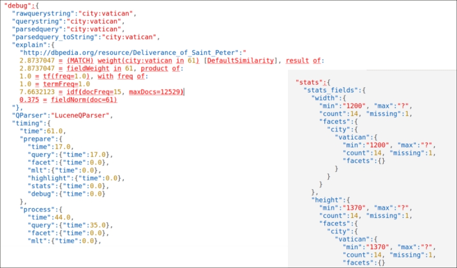
- In the following screenshot you'll see them in action, stats on the left side, and debug on the right side:
- If you are curious about what kind of information you can obtain with the same query using the pseudo field
[explain], it's easy to test it using the following command:>> curl -X GET 'http://localhost:8983/solr/paintings/select?q=city:vatican&rows=1&stats=true&stats.field=width&stats.field=height&stats.facet=city&fl=[explain+style=nl]&indent=true&wt=json' - In the following screenshot, you'll see it in action:
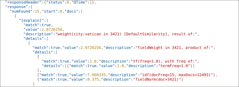
- This screenshot clearly shows how the
[explain]pseudo field is not directly related todebugorstats, but it can still be used to debug the actual parsing. We will look at query parsing in detail using both of them, and the analogous explain section exposed by the debug component, in the next sections, using more complex and interesting queries.
On the left side of the first screenshot, we can recognize different stages in the query parsing and execution, from the text typed by the user (rawquerystring) to the explain section where we can look at the internally expanded syntax. We will use the syntax later with more complex examples; remember that the explain section will include a line for every row (in this case, rows=1, so one line). In addition to this information, we can obtain an explicit reference to the parser used for the query (QParser, in this case is the default Lucene one) and to the time spent for the execution of the various components.
The stats component in the second example (on the right side of the first screenshot) provides a sequence of values about a specific field; for example, stats.field=width is used to show statistics about the values for the specific field width (minimum, maximum, how many are there, how many are missing, and so on), and stats.facet=city can be used to enable faceting of statistical values over this field. It's easy at the moment to think about stats.facet as a way to add statistics of the terms on a per-field basis. Every facet in this example will represent statistics starting from a particular field, used as our central point of interest.
For example, searching for paintings and asking for statistics about them with a facet attribute on city can be done as follows:
>> curl -X GET 'http://localhost:8983/solr/paintings/select?q=abstract:portrait&rows=0&stats=true&stats.field=width&stats.field=height&stats.facet=city&wt=json&indent=true&json.nl=map'
The preceding command will give us many lines in the facet section of every stats section, one for each term in the city field (the terms are actually indexed depending on the particular chosen tokenizers). Note also how these results are independent of the number of rows as they refer to general statistics for fields in a specific schema, and we can use them to gain a wide view of the data, starting from a specific point.
The usage of the pseudo field fl=[explain+style=nl] actually gives us some more structured visualization of the debug metadata about the terms in the result, as you can see in the second screenshot. We will use these kinds of results in particular for more complex queries, but you can also combine the two different results if you want to compare them by simply adding both the parameters into your requests.
The Lucene query parser has been extended in Solr to take care of some recurring use cases. For example, it is possible to provide more flexibility for ranged queries, leaving them open ended, by using a * character to indicate that there is no lower or upper limit, or explicitly specify queries that must not include a specific term. We can look at the differences between the Lucene parser and the Solr default parser, based on Lucene: http://wiki.apache.org/solr/SolrQuerySyntax.
Moreover, there are pseudo fields that are used as fields but are actually computed by some functions. This way we can, for example, embed subqueries (with the _query_:text-of-subquery syntax) and function queries (with the _val_:text-of-functionquery syntax). You can easily note that _field_ denotes a pseudo field or an internal field, as we have already seen for _version_.
For a real-world application, however, we need to manage queries that cannot contain special operators, as they can be too much complex for common users, and we'd like to have some more robust parsing over errors and typos in the queries. While it is always possible to define some kind of pre/post processing of a query at application level, there are two more query parsers that we can use because they are designed specifically for common users: Dismax and Edismax.