
CHAPTER 10
UNDERSTANDING STUDIES AND SURVEYS OF COMPUTER CRIME
M. E. Kabay
10.1.1 Value of Statistical Knowledge Base
10.1.2 Limitations on Our Knowledge of Computer Crime
10.1.3 Limitations on the Applicability of Computer Crime Statistics
10.2 BASIC RESEARCH METHODOLOGY
10.2.1 Some Fundamentals of Statistical Design and Analysis
10.2.2 Research Methods Applicable to Computer Crime
10.1 INTRODUCTION.
This chapter provides guidance for critical reading of research results about computer crime. It will also alert designers of research instruments who may lack formal training in survey design and analysis to the need for professional support in developing questionnaires and analyzing results.
10.1.1 Value of Statistical Knowledge Base.
Security specialists are often asked about computer crime; for example, customers want to know who is attacking which systems, how often, using what methods. These questions are perceived as important because they bear on the strategies of risk management; in theory, in order to estimate the appropriate level of investment in security, it would be helpful to have a sound grasp of the probability of different levels of damage. Ideally, one would want to evaluate an organization's level of risk by evaluating the experiences of other organizations with similar system and business characteristics. Such comparisons would be useful in competitive analysis and in litigation over standards of due care and diligence in protecting corporate assets.
10.1.2 Limitations on Our Knowledge of Computer Crime.
Unfortunately, in the current state of information security, no one can give reliable answers to such questions. There are two fundamental difficulties preventing us from developing accurate statistics of this kind. These difficulties are known as the problems of ascertainment.
10.1.2.1 Detection.
The first problem is that an unknown number of crimes of all kinds are undetected. For example, even outside the computer crime field, we do not know how many financial frauds are being perpetrated. We do not know because some of them are not detected. How do we know they are not detected? Because some frauds are discovered long after they have occurred. Similarly, computer crimes may not be detected by their victims but may be reported by the perpetrators.
In a landmark series of tests at the Department of Defense (DoD), the Defense Information Systems Agency found that very few of the penetrations it engineered against unclassified systems within the DoD seem to have been detected by system managers. These studies were carried out from 1994 through 1996 and attacked 38,000 systems. About two-thirds of the attacks succeeded; however, only 4 percent of these attacks were detected.1
A commonly held view within the information security community is that only one-tenth or so of all the crimes committed against and using computer systems are detected.
10.1.2.2 Reporting.
The second problem of ascertainment is that even if attacks are detected, few seem to be reported in a way that allows systematic data collection. This commonly held belief is based in part on the unquantified experience of information security professionals who have conducted interviews of their clients; it turns out that only about 10 percent of the attacks against computer systems revealed in such interviews were ever reported to any kind of authority or to the public. The DoD studies mentioned earlier were consistent with this belief; of the few penetrations detected, only a fraction of 1 percent were reported to appropriate authorities.
Given these problems of ascertainment, computer crime statistics generally should be treated with skepticism.
10.1.3 Limitations on the Applicability of Computer Crime Statistics.
Generalizations in this field are difficult to justify. Even if we knew more about types of criminals and the methods they use, it still would be difficult to have the kind of actuarial statistic that is commonplace in the insurance field. For example, the establishment of uniform building codes in the 1930s in the United States led to the growth in fire insurance as a viable business. With official records of fires in buildings that could be described using a standard typology, statistical information began to provide an actuarial basis for using probabilities of fires and associated costs to calculate reasonable insurance rates.
In contrast, even if we had access to accurate reports, it would be difficult to make meaningful generalizations about vulnerabilities and incidence of successful attacks for the information technology field. We use a bewildering variety and versions of processors, operating systems, firewalls, encryption, application software, backup methods and media, communications channels, identification, authentication, authorization, compartmentalization, and operations.
How would we generalize from data about the risks at (say) a mainframe-based network running Multiple Virtual Systems (MVS) in a military installation to the kinds of risks faced by a UNIX-based intranet in an industrial corporation, or to a Windows New Technology (NT)-based Web server in a university setting? There are so many differences among systems that if we were to establish a multidimensional analytical table where every variable was an axis, many cells would likely contain no or only a few examples. Such sparse matrices are notoriously difficult to use in building statistical models for predictive purposes.
10.2 BASIC RESEARCH METHODOLOGY.
This is not a chapter about social sciences research. However, many discussions of computer crime seem to take published reports as gospel, even though these studies may have no validity whatsoever. In this short section, we look at some fundamentals of research design so that readers will be able to judge how much faith to put in computer crime research results.
10.2.1 Some Fundamentals of Statistical Design and Analysis.
The way in which a scientist or reporter represents data can make an enormous difference in the readers' impressions.
10.2.1.1 Descriptive Statistics.
Suppose three companies reported these losses from penetration of their computer systems: $1M, $2M, and $6M. We can describe these results in many ways. For example, we can simply list the raw data; however, such lists could become unacceptably long as the number of reports increased, and it is hard to make sense of the raw data.
We could define classes such as “2 million or less” and “more than 2 million” and count how many occurrences there were in each class:
| Class | Freq |
| ≤ $2M | 2 |
| > $2M | 1 |
Alternatively, we might define the classes with finer granularity as < $1M, ≥ $1M but < $2M, and so on; such a table might look like this:
| Class | Freq |
| < $1M | 0 |
| ≥ $1M & < $2M | 1 |
| ≥ $2M & < $3M | 1 |
| ≥ $3M & < $4M | 0 |
| ≥ $4M & < $5M | 0 |
| ≥ $5M & < $6M | 0 |
| ≥ $6 | 1 |
Notice how the definition of the classes affects perception of the results: The first table gives the impression that the results are clustered around $2M and gives no information about the upper or lower bounds.
10.2.1.1.1 Location.
One of the most obvious ways we describe data is to say where they lie in a particular dimension. The central tendency of our three original data ($1M, $2M, and $6M) can be represented in various ways; for example, two popular measures are
- Arithmetic mean or average = $(1+2+6)M/3 = $3M
- Median (the middle of the sorted list of losses) = $2M
Note that if we tried to compute the mean and the median from the first table (with its approximate classes), we would get the wrong value. Such statistics should be computed from the original data, not from summary tables.
10.2.1.1.2 Dispersion.
Another aspect of our data that we frequently need is dispersion—that is, variability. The simplest measure of dispersion is the range: the difference between the smallest and the largest value we found; in our example, we could say that the range was from $1M to $6M or that it was $5M. Sometimes the range is expressed as a percentage of the mean; then we would say that the range was 5/3 = 1.6… or ~167 percent.
The variance (σ2) of these particular data is the average of the squared deviations from the arithmetic mean; the variance of the three numbers would be σ2 = (1−3)2 + (2−3)2 + (6−3)2/3 = (4+1+9)/3 ≈ 4.67.
The square root of the variance (σ) is called the standard deviation and is often used to describe dispersion. In our example, σ = √4.67 ≈ 2.16.
Dispersion is particularly important when we compare estimates about information from different groups. The greater the variance of a measure, the more difficult it is to form reliable generalizations about an underlying phenomenon, as described in the next section.
10.2.1.2 Inference: Sample Statistics versus Population Statistics.
We can accurately describe any data using descriptive statistics; the question is what we then do with those measures.
Usually we expect to extend the findings in a sample or subset of a population to make generalizations about the population. For example, we might be trying to estimate the losses from computer crime in commercial organizations with offices in the United States and with more than 30,000 employees. Or perhaps our sample would represent commercial organizations with offices in the United States and with more than 30,000 employees and whose network security staff was willing to respond to a survey questionnaire.
In such cases, we try to infer the characteristics of the population from the characteristics of the sample. Statisticians say that we try to estimate the parametric statistics by using the sample statistics.
For example, we estimate the parametric (population) variance (usually designated σ2) by multiplying the variance of the sample by n/(n−1). Thus we would say that the estimate of the parametric variance (s2) in our sample would be s2 = 4.67 * 3/2 = 7. The estimate of the parametric standard deviation (s) would be s = √7 ≈ 2.65.
10.2.1.3 Hypothesis Testing.
Another kind of inference that we try to make from data is hypothesis testing. For example, suppose we were interested in whether there was any association between the presence or absence of firewalls and the occurrence of system penetration. We can imagine collecting these data about penetrations into systems with or without firewalls:
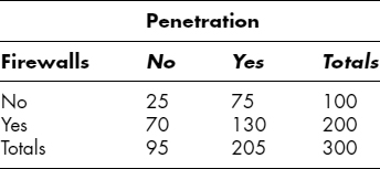
We would frame the hypothesis (the null hypothesis, sometimes represented as H0) that there was no relationship between the two independent variables, penetration and firewalls, and test that hypothesis by performing a test of independence of these variables. In our example, a simple chi-square test of independence would give a test statistic of χ2[1] = 2.636. If there really were no association between penetration and firewalls in the population of systems under examination, the parametric value of this statistic would be zero. In our imaginary example, we can show that such a large value (or larger) of χ2[1] would occur in only 10.4 percent of the samples taken from a population where firewalls had no effect on penetration. Put another way, if we took many samples from a population where the presence of firewalls was not associated with any change in the rate of penetration, we would see about 10.4 percent of those samples producing χ2[1] statistics as large as or larger than 2.636.
Statisticians have agreed on some conventions for deciding whether a test statistic deviates enough from the value expected under the null hypothesis to warrant inferring that the null hypothesis is wrong. Generally we describe the likelihood that the null hypothesis is true—often shown as p(H0)—in this way:
- When p(H0) > 0.05, we say the results are not statistically significant (often designated with the symbols ns);
- When 0.05 ≥ p(H0) > 0.01, the results are described as statistically significant (often designated with the symbol *);
- When 0.01 ≥ p(H0) > 0.001, the results are described as highly statistically significant (often designated with the symbols **);
- When p(H0) ≤ 0.001, the results are described as extremely statistically significant (often designated with the symbols ***).
10.2.1.4 Random Sampling, Bias, and Confounded Variables.
The most important element of sampling is randomness. We say that a sample is random or randomized when every member of the population we are studying has an equal probability of being selected. When a population is defined one way but the sample is drawn nonrandomly, the sample is described as biased. For example, if the population we are studying was designed to be, say, all companies worldwide with more than 30,000 full-time employees, but we sampled mostly from such companies in the United States, the sample would be biased toward U.S. companies and their characteristics. Similarly, if we were supposed to be studying security in all companies in the United States with more than 30,000 full-time employees but we sampled only from those companies that were willing to respond to a security survey, we would be at risk of having a biased sample.
In this last example, involving studying only those who respond to a survey, we say that we are potentially confounding variables: We are looking at people-who-respond-to-surveys and hoping they are representative of the larger population of people from all companies in the desired population. But what if the people who are willing to respond are those who have better security and those who do not respond have terrible security? Then responding to the survey is confounded with quality of security, and our biased sample could easily mislead us into overestimating the level of security in the desired population.
Another example of how variables can be confounded is comparisons of results from surveys carried out in different years. Unless exactly the same people are interviewed in both years, we may be confounding individual variations in responses with changes over time; unless exactly the same companies are represented, we may be confounding differences among companies with changes over time; if external events have led people to be more or less willing to respond truthfully to questions, we may be confounding willingness to respond with changes over time. If the surveys are carried out with different questions or used by different research groups, we may be confounding changes in methodology with changes over time.
10.2.1.5 Confidence Limits.
Because random samples naturally vary around the parametric (population) statistics, it is not very helpful to report a point estimate of the parametric value. For example, if we read that the mean damage from computer crimes in a survey was $180,000 per incident, what does that imply about the population mean?
To express our confidence in the sample statistic, we calculate the likelihood of being right if we give an interval estimate of the population value. For example, we might find that we would have a 95 percent likelihood of being right in asserting that the mean damage was between $160,000 and $200,000. In another sample, we might be able to narrow these 95 percent confidence limits to $175,000 and $185,000.
In general, the larger the sample size, the narrower the confidence limits will be for particular statistics.
The calculation of confidence limits for statistics depends on some necessary assumptions:
- Random sampling
- A known error distribution (usually the Normal distribution—sometimes called a Gaussian distribution)
- Equal variance at all values of the measurements
If any of these assumptions is wrong, the calculated confidence limits for our estimates will be wrong; that is, they will be misleading. There are tests of these assumptions that analysts should carry out before reporting results; if the data do not follow Normal error distributions, sometimes one can apply normalizing transformations.
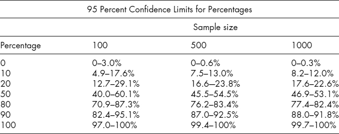
In particular, percentages do not follow a Normal distribution. Here is a reference table of confidence limits for various percentages in a few representative sample sizes.
10.2.1.6 Contingency Tables.
One of the most frequent errors in reporting results of studies is to provide only part of the story. For example, one can read statements such as “Over 70 percent of the systems without firewalls were penetrated last year.” Such a statement may be true, but it cannot be interpreted correctly as meaning that systems with firewalls were necessarily more or less vulnerable to penetration than systems without firewalls. The statement is incomplete; to make sense of it, we need the other part of the implied contingency table—the percentage of systems with firewalls that were penetrated last year—before making any assertions about the relationship between firewalls and penetrations. Compare, for example, these two hypothetical tables:
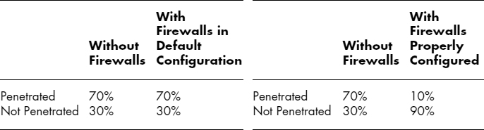
In both cases, someone could say that “70 percent of the systems without firewalls were penetrated,” but the implications would be radically different in the two data sets. Without knowing the right-hand column, the original assertion would be meaningless.
10.2.1.7 Association versus Causality.
Continuing our example with rates of penetration, another error that untrained people often make when studying statistical information is to mistake association for causality. Imagine that a study showed that a lower percentage of systems with fire extinguishers was penetrated than systems without fire extinguishers and that this difference was statistically highly significant. Would such a result necessarily mean that fire extinguishers caused the reduction in penetration? No. We know that it is far more reasonable to suppose that the fire extinguishers were installed in organizations whose security awareness and security policies were more highly developed than in the organizations where no fire extinguishers were installed. In this imaginary example, the fire extinguishers might actually have no causal effect whatever on resistance to penetration. This result would illustrate the effect of confounding variables: presence of a fire extinguisher with state of security awareness and policies.
10.2.1.8 Control Groups.
Finally, to finish our penetration example, one way to distinguish between association and causality is to control for variables. For example, one could measure the state of security awareness and policy as well as the presence or absence of fire extinguishers and make comparisons only among groups with the same level of awareness and policy. There are also statistical techniques for mathematically controlling for differences in such independent variables.
10.2.1.9 A Priori versus a Posteriori Testing.
Amateurs or beginners sometimes forget the principle of random sampling that underlies all statistical inference (see Section 10.2.1.4). None of the hypothesis tests or confidence limit calculations work if a sample is not random. For example, if someone is wandering through a supermarket and notices that Granny Smith apples seem to be bigger than Macintosh apples, selecting a sample—even a random sample—of the apples that specifically gave rise to the hypothesis will not allow reliable computations of probability that the applies have the same average weight. The problem is that those particular applies would not have been sampled at all had the observer not been moved to formulate the hypothesis. So even if a particular statistical comparison produces a sample statistic that appears to have a probability of, say, 0.001, it is not possible to know how much the sampling deviated from randomness.
Applying statistical tests to data after one notices an interesting descriptive value, comparison, or trend is known as a posteriori testing. Formulating a hypothesis, obtaining a random sample, and computing the statistics and probabilities in accordance with the assumptions of those statistics and probabilities is known as a priori testing.
A well-used example of the perils of a posteriori testing is the unfortunate habit of searching through sequences of results such as long strings of guesses collected in student tests of paranormal abilities and calculating statistical values on carefully selected subsets of the strings. These a posteriori tests are then presented as if they were a priori and cause great confusion and arguments, such as: “Look, even though the overall proportion of correct guesses was (say) 50.003 percent in this run of <some very large number> guesses, there was a run of <much smaller number> guesses that were correct <any value greater than 50 percent> of the time! The probability of such a result by chance is <very small number>. That proves that there was a real effect of <whatever the treatment was>.” Unfortunately, a long series of numbers can produce any desired nonrandom-looking string; there are even tests known as runs tests that can help a researcher evaluate the nonrandomness of such occurrences.
In practical terms, statisticians have established a convention for limiting the damaging effects of a posteriori testing: Use the 0.001 level of probability as the equivalent of the minimum probability of the null hypothesis. This custom makes it far less likely that an a posteriori comparison will trick the user into accepting what is in fact a random variation that caught someone's eye.
The best solution to the bias implicit in a posteriori testing is to use a completely new sample for the comparison. In the apple example, one could ask the store manager for new, unobserved, and randomly selected batches of both types of applies. The comparison statistics would then be credible and could be expected to follow the parametric distribution underlying calculations of probability of the null hypothesis. The populations from which these apples were selected still would have to be carefully determined. Would the populations be apples at this particular store? For this particular chain? For this particular region of the country or of the world?
10.2.2 Research Methods Applicable to Computer Crime
10.2.2.1 Interviews.
Interviewing individuals can be illuminating. In general, interviews provide a wealth of data that are unavailable through any other method. For example, one can learn details of computer crime cases or motivations and techniques used by computer criminals. Interviews can be structured (using precise lists of questions) or unstructured (allowing the interviewer to respond to new information by asking additional questions at will).
Interviewers can take notes or record the interviews for later word-for-word transcription. In unstructured interviewers, skilled interviewers can probe responses to elucidate nuances of meaning that might be lost using cruder techniques such as surveys. Techniques such as thematic analysis can reveal patterns of responses that can then be examined using exploratory data analysis.2 Thematic analysis is a technique for organizing nonquantitative information without imposing a preexisting framework on the data; exploratory data analysis uses statistical techniques to identify possibly interesting relationships that can be tested with independently acquired data. Such exploratory techniques can correctly include a posteriori testing as described in Section 10.2.1.9, but the results are used to propose further studies that can use a priori tests for the best use of resources.
10.2.2.2 Focus Groups.
Focus groups are like group interviews. Generally the facilitator uses a list of predetermined questions and encourages the participants to respond freely and to interact with each other. Often the proceedings are filmed from behind a one-way mirror for later detailed analysis. Such analysis can include nonverbal communications, such as facial expressions and other body language as the participants speak or listen to others speak about specific topics.
10.2.2.3 Surveys.
Surveys consist of asking people to answer a fixed series of questions with lists of allowable answers. They can be carried out face to face or by distributing and retrieving questionnaires by telephone, mail, fax, and e-mail. Some questionnaires have been posted on the Web.
The critical issue when considering the reliability of surveys is self-selection bias—the obvious problem that survey results include only the responses of people who agreed to participate. Before basing critical decisions on survey data, it is useful to find out what the response rate was; although there are no absolutes, in general, we tend to trust survey results more when the response rate is high. Unfortunately, response rates for telephone surveys are often less than 10 percent; response rates for mail and e-mail surveys can be less than 1 percent. It is very difficult to make any case for random sampling under such circumstances, and all results from such low-response-rate surveys should be viewed as indicating the range of problems or experiences of the respondents rather than as indicators of population statistics.
Regarding Web-based surveys, there are two types from a statistical point of view: those using strong identification and authentication and those that do not. Those that do not are vulnerable to fraud, such as repeated voting by the same individuals. Those that provide individual universal resource locators (URLs) to limit voting to one per person nonetheless suffer from the same problems of self-selection bias as any other survey.
10.2.2.4 Instrument Validation.
Interviews and other social sciences research methodologies can suffer from a systematic tendency for respondents to shape their answers to please the interviewer or to express opinions that may be closer to the norm in whatever group they see themselves. Thus, if it is well known that every organization ought to have a business continuity plan, some respondents may misrepresent the state of their business continuity planning to look better than they really are.
In addition, survey instruments may distort responses by phrasing questions in a biased way; for example, the question “Does your business have a completed business continuity plan?” may have a more accurate response rate than the question “Does your business comply with industry standards for having a completed business continuity plan?” The latter question is not neutral and is likely to increase the proportion of “yes” answers.
The sequence of answers may bias responses; exposure to the first possible answers can inadvertently establish a baseline for the respondent. For example, a question about the magnitude of virus infections might ask:
In the last 12 months, has your organization experienced total losses from virus infections of
- (a) $1M or greater;
- (b) less than $1M but greater than or equal to $100,000;
- (c) less than $100,000;
- (d) none at all?
To test for bias, the designer can create versions of the instrument in which the same information is obtained using the opposite sequence of answers:
In the last 12 months, has your organization experienced total losses from virus infections of
- (a) none at all;
- (b) less than $100,000;
- (c) less than $1M but greater than or equal to $100,000;
- (d) $1M or greater?
The sequence of questions can bias responses; having provided a particular response to a question, the respondent will tend to make answers to subsequent questions about the same topic conform to the first answer in the series. To test for this kind of bias, the designer can create versions of the instrument with questions in different sequences.
Another instrument validation technique inserts questions with no valid answers or with meaningless jargon to see if respondents are thinking critically about each question or merely providing any answer that pops into their heads. For example, one might insert the nonsensical question, “Does your company use steady-state quantum interference methodologies for intrusion detection?” into a questionnaire about security and invalidate the results of respondents who answer yes to this and other diagnostic questions.
Finally, independent verification of answers provides strong evidence of whether respondents are answering truthfully. However, such intrusive investigations are rare.
10.3 SUMMARY.
In summary, all studies about computer crime should be studied carefully before we place reliance on their results. Some basic take-home questions about such research:
- What is the population we are sampling?
- Keeping in mind the self-selection bias, how representative of the wider population are the respondents who agreed to participate in the study or survey?
- How large is the sample?
- Are the authors testing for the assumptions of randomness, normality, and equality of variance before reporting statistical measures?
- What are the confidence intervals for the statistics being reported?
- Are comparisons confounding variables?
- Are correlations being misinterpreted as causal relations?
- Were the test instruments validated?
10.4 FURTHER READING
Textbooks
If you are interested in learning more about survey design and statistical methods, you can study any elementary textbook on the social sciences statistics. Here are some sample titles:
Babbie, E. R., F. S. Halley, and J. Zaino. Adventures in Social Research: Data Analysis Using SPSS 110/11.5 for Windows, 5th ed. Pine Forge Press, 2003.
Bachman, R., and R. K. Schutt. The Practice of Research in Criminology and Criminal Justice, 3rd ed. Sage Publications, 2007.
Chambliss, D. F., and R. K. Schutt. Making Sense of the Social World: Methods of Investigation, 2nd ed. Pine Forge Press, 2006.
Sirkin, R. M. Statistics for the Social Sciences, 3rd ed. Sage Publications, 2005.
Web Sites
Creative Research Systems, “Survey Design,” www.surveysystem.com/_sdesign.htm.
New York University, “Statistics & Social Science,” www.nyu.edu/its/socsci/statistics.html
StatPac, “Survey & Questionnaire Design,” www.statpac.com/surveys/.
10.5 NOTES
1. GAO 91996) “Computer Attacks at Department of Defense Pose Increasing Risks.” General Accounting Office Report to Congressional Requesters GAO/AIMD-98-84 (May 1996). P.19
2. M. E. Kabay, “CATA: Computer-Aided Thematic Analysis,” 2006. Available at www2.norwich.edu/mkabay/methodology/CATA.pdf with narrated lectures at www2.norwich.edu/mkabay/methodology/index.htm.