CHAPTER 62

RISK ASSESSMENT AND RISK MANAGEMENT

Robert V. Jacobson

62.1 INTRODUCTION TO RISK MANAGEMENT

62.1.1 What Is Risk?

62.1.2 What Is Risk Management?

62.1.3 Applicable Standards

62.1.4 Regulatory Compliance and Legal Issues

62.2 OBJECTIVE OF A RISK ASSESSMENT

62.3 LIMITATIONS OF QUESTIONNAIRES IN ASSESSING RISKS

62.4 MODEL OF RISK

62.4.1 Two Inconsequential Risk Classes

62.4.2 Two Significant Risk Classes

62.4.3 Spectrum of Real-World Risks

62.5 RISK MITIGATION

62.5.1 ALE Estimates Alone Are Insufficient

62.5.2 What a Wise Risk Manager Tries to Do

62.5.3 How to Mitigate Infrequent Risks

62.5.4 ROI-Based Selection Process

62.5.5 Risk Assessment/Risk Management Summary

62.6 RISK ASSESSMENT TECHNIQUES

62.6.1 Aggregating Threats and Loss Potentials

62.6.2 Basic Risk Assessment Algorithms

62.6.3 Loss Potential

62.6.4 Risk Event Parameters

62.6.5 Threat Effect Factors, ALE, and SOL Estimates

62.6.6 Sensitivity Testing

62.6.7 Selecting Risk Mitigation Measures

62.7 SUMMARY

62.8 FURTHER READING

62.9 NOTES

62.1 INTRODUCTION TO RISK MANAGEMENT

62.1.1 What Is Risk?

There is general agreement in the computer security community with the common dictionary definition: “the possibility of suffering harm or loss.” The definition shows that there are two parts to risk: the possibility that a risk event will occur, and the harm or loss that results from occurrences of risk events. Consequently, the assessment of risk requires consideration of both factors: the frequency of threat events that cause losses, and the loss each such event causes. The product of the two factors, frequency and loss, is a quantitative measure of risk; for example, we might express a risk as an annualized loss expectancy (discussed in Section 62.4.3) of, say, “$100,000 per year.” Risk is managed by taking actions that recognize and reduce these two factors.

Management of risk is important to the design, implementation, and operation of information technology (IT) systems because IT systems are increasingly an essential part of the operation of most organizations. As a result, both the size of the potential harm or loss and the possibility of arisk event occurring are increasing. In extreme cases, a risk loss may be large enough to destroy an organization. If an organization's risk management program is deficient in some area, the organization may suffer excessive harm or loss, but at the same time, the organization may be wasting resources on ineffective, excessive, or misdirected mitigation measures in other areas.

62.1.2 What Is Risk Management?

This chapter discusses risk management with special emphasis on two aspects of risk management: risk assessment and risk mitigation. Exhibit 62.1 suggests that risk management can be thought of as a four-step process.

The first step in managing the risks to an IT system is to identify and assess the risks quantitatively. The second step is to use the product of the risk assessment to identify the optimum set of risk measures.¹ In this context, “optimum” means making mitigation the best use of the resources available. Because no organization has infinite resources, risk management requires allocating finite resources, by selecting from the broad range of IT risk mitigation measures, the optimum set. Since the resources being allocated are measured quantitatively in monetary terms, the risks must likewise be measured in monetary terms. A CIO can hardly expect to go to the CFO and announce that the risk assessment has identified a “High” risk, so a “High” security budget will be needed to address the risk. This issue is discussed in more detail in Section 62.4.3.

The third step, security operations, is to perform the ongoing, daily activities necessary for the effective functioning of the risk management measures. Finally, the fourth step, security auditing, is to evaluate the effectiveness of IT security operations and to detect changing conditions that require a reassessment of risks, the implementation of new mitigation measures, or modifications to the security management program. Daily security management tasks and IT auditing are discussed elsewhere in this Handbook (see, e.g., Chapters 23, 27, 40, 47, 52, 53, and 54), so this chapter will confine itself to the first two steps: risk assessment and risk mitigation.

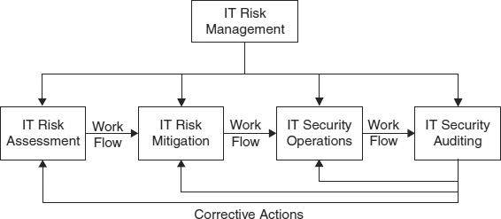
EXHIBIT 62.1 Four IT Risk Management Activities

62.1.3 Applicable Standards.

There are two widely cited standards that address IT system risks: ISO/IEC 17799² (ISO 17799) and GTAG Information Technology Controls³ (GTAG-ITC).

In 1995 the British Standards Institute published BS7799 entitled Information Security Management Systems—Specification with Guidance for Use. It is described as defining a six-step process:

1. Define the scope of the information security management system (ISMS).
2. Define a security policy.
3. Undertake a risk assessment/analysis.
4. Manage the risk.
5. Select control objectives and the actual controls to be implemented/applied.
6. Prepare a statement of applicability.

In 2000 BS7799 became ISO 17799. Although ISO 17799 offers a wealth of advice, its treatment of risk is not sharply focused. ISO 17799 Section 0.4—What Is Information Security? defines information security as “the protection of information from a wide range of threats in order to ensure business continuity, minimize business risk, and maximize return on investments and business opportunities.” Although the definition includes “business continuity” as an objective, it focuses on “information” while it ignores threats to the operation of IT facilities such as fire, hardware failures, power outages, and so on that may not directly affect information. Since both information and physical facilities are required to perform the IT functions that support the operation of the parent organization, it is essential to consider both to manage risks effectively. Here is a simple example: If physical access controls do not protect data storage devices against improper physical access, control over access to stored data is lost regardless of logical access controls (e.g., passwords that may be in place). Thus, when reading ISO 17799, one should mentally translate the phrase “information security” as “IT system risk management,” and take note of missing topics.

Section 0.4—Assessing Security Risks makes these sound observations: “Expenditure on controls needs to be balanced against the business harm likely to result from security failures.” and “The results of the risk assessment will help to guide and determine the appropriate management action and priorities for managing information risks, and for implementing controls selected to protect against these risks.” In section 2.9, ISO 17799 replaces the dictionary definition of risk quoted in Section 62.1.1 with this: “[risk is the] combination of the probability of an event and its consequence.” If the word “combination” means “product,” then what is being defined is annualized loss expectancy (ALE), a far more accurate term. ISO 17799, Section 4—Risk Assessment and Treatment, begins with this assertion: “Risk assessments should identify, quantify, and prioritize risks against criteria for risk acceptance and objectives relevant to the organization.” These two qualitative criteria, risk acceptance and corporate objectives, are incompatible with a quantitative risk assessment, and the assertion is at cross-purposes with section 0.4, as quoted. Finally, ISO 17799, Section 14—Business Continuity Management, similarly loses sight of cost-benefit as the only valid criterion for defining a business continuity program. In summary, although this ISO standard offers many security topics for consideration, its emphasis on information security results in a fuzzy treatment of risk management.

In October 2005, ISO 17799 became ISO 27001 as a part of an ISO plan to devote the 27000 series of standards for “information security matters.” ISO 27001 is described as a “standard” for “information security management systems.” Despite the name, it is not a standard. It is actually a guideline for IT system security management that covers all aspects of IT system operations. In effect, it spans the third and fourth boxes in Exhibit 62.1.

The GTAG-ITC guide (Global Technology Audit Guide—Information Technology Controls), published by the Institute of Internal Auditors, addresses risk management from the viewpoint of an internal auditor but is a useful source of information for IT risk managers because of its detailed discussion of roles and missions, and of IT controls. Section 8—Analyzing Risk discusses specifics of risk management. Section 8.1 includes this sensible comment: “However, each control has a specific cost that may not be justified in terms of cost-effectiveness…. Furthermore, no list of controls is universally applicable.” This says very clearly that IT controls, even those recommended by auditors, should pass a cost-effectiveness test before being selected for implementation. Section 8.2.4—Performing Risk Analysis describes the risk management process succinctly but has the same conceptual error as ISO 17799 in that it refers to “assets” but ignores processes and the facilities needed to perform them.

The reference to risk management measures as “controls” may suggest that actions that are not “controls”—for example, insurance or business continuity plans—are not a part of the risk management program. This is the reason why we use the term “risk management measures” here, not “controls.”

62.1.4 Regulatory Compliance and Legal Issues.

Increasing regulatory and legal issues are impacting risk management, most notably the Sarbanes-Oxley Act. More and more corporate officials are being sent to jail for infractions. As a result, it is not surprising that there may be an overreaction to compliance regulations with excessive measures being recommended by auditors. Whenever implementation of a compliance recommendation does not include a cost justification, and the implementation cost is material, it may be a candidate for a simple risk analysis like this:

1. What effect does the recommended measure have on the probability of noncompliance? In other words, what will be the difference in the likely loss experience with and without the recommended measure?
2. Does this difference compare favorably with the cost to implement and maintain the recommended measure?

There are several points to be made:

• If the cost-benefit is marginal or negative, consideration should be given to alternate (and lower cost) ways to achieve the same end result.
• If the cost-benefit is strongly negative, consideration should be given to dropping the recommendation.
• Under no circumstances should an organization deliberately break the law.

For more about these issues, refer to Chapter 65 in this Handbook.

62.2 OBJECTIVE OF A RISK ASSESSMENT.

This Handbook describes the pros and cons of a wide range of security measures that can be applied to an IT system. However, no organization has unlimited resources, and so it is necessary to decide which measures should be implemented.⁴ It would be convenient if there were a set of security standards that applied equally to all IT systems, but as the GTAG-ITC guidelines cited in Section 62.1.3 note, this is not the case for two basic reasons:

1. Each IT system has its own particular risk environment.
2. Each IT system has a unique workload. Although two or more IT systems may perform the same list of functions, it is highly unlikely that the systems will have exactly the same level of activity for each of the functions, and so the cost of lost data and service interruptions will not be the same.

Because of these differences, each IT system will have unique security requirements.⁵ These two factors correspond to the two elements in the definition of risk:

1. The risk environment determines the possibility of experiencing harm or loss.
2. The characteristics of the system workload, and the associated IT system assets, determine the magnitude of the harm or loss.

The objective of a risk assessment is to generate information about risk exposures and the potential for loss associated with the workload in order to estimate the ALE of the IT system under current conditions. This estimate is needed to optimize the subsequent risk mitigation decisions and to validate decisions about existing security measures. In this context, optimize means to allocate the organization's resources to those actions that will yield the best overall performance. It would be suboptimum to spend $10,000 to avert $1,000 in expected losses. To avoid such wasteful expenditures, one must be able to estimate quantitatively both expected losses⁶ and the effect of proposed mitigation measures. For this reason, in all but the simplest situations, a risk assessment must produce a quantitative, monetary measure of risk, so that (1) risks can be compared with one another on a common basis and (2) the cost of risk mitigation measures can be related to the risks they are meant to address. Assessing a risk as “high,” “unacceptable,” or in other qualitative terms does not provide the information needed to support decisions to implement risk mitigation measures, which will always have quantitative implementation costs.

Exhibit 62.2 shows why a quantitative estimate of ALE is an essential element in the optimization of the strategy. A sum of money has been budgeted for IT risk management for next year. A risk management measure is selected and implemented, and so funds are expended. The implementation is expected to reduce one or more risk factors. As a result, we expect future risk losses will be reduced, and funds will be saved. By comparing the present values of the funds expended now and those saved in the future, we can estimate the return on investment (ROI) of the implemented measure. The goal is to maximize the ROI and to avoid risk management measures with small or negative ROIs. This is the essential character of businesslike IT system risk management. However, it is evident that we must be able to make credible estimates of expected risk losses under both current conditions and under the assumption that a proposed risk management measure has been implemented to optimize our risk management strategy. It may be suggested that quantitative assessment of risk is “too complicated” and so a simpler, qualitative method can be used instead. However, the complexity is inherent in risk itself, and any “simple” assessment technique will be inherently weak and potentially misleading. This topic is discussed in more detail in Section 62.4.3.

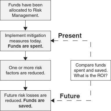
EXHIBIT 62.2 Evaluating an IT System Security Strategy

62.3 LIMITATIONS OF QUESTIONNAIRES IN ASSESSING RISKS.

One may be tempted to think of a “security questionnaire” or checklist as a valid risk assessment, but even if the checklist seems to be authoritative because it is automated, this is not the case. Typical questionnaires evaluate, to some extent, the risk environment but not expected loss. At best, a questionnaire can only compare the target of the questionnaire with a security standard implicit in the individual questions. Questionnaires do not meet the objective of a risk assessment, because the answers to a questionnaire will not support optimized selection of risk mitigation measures. The most a well-designed questionnaire can do is to identify potential risk areas, and so it can be of help in scoping and focusing a quantitative risk assessment.

Questionnaires suffer from several other shortcomings:

• The author of a question and the person who is answering the question may have different understandings of the meanings of key words. As a result, an answer may not match the intent of a question.
• Questions tend to be binary, but most answers are inherently quantitative. For example, consider the binary question “Do users comply with password policy?” Although the anticipated answer is either yes or no, a meaningful answer is likely to be much more complicated because each user will have a unique pattern of compliance. Some users will make every effort to be 100 percent compliant, some will make every effort to circumvent the policy, and the remaining users will comply to a greater or lesser extent. Note also that the question does not attempt to evaluate the appropriateness of the policy.
• Because questionnaires are inherently “open loop,” and because of the binary answer issue just discussed, questionnaires tend to miss important information that would be elicited by a risk analyst who interacts directly with respondents and responds to a quantitative answer with a new question.⁷

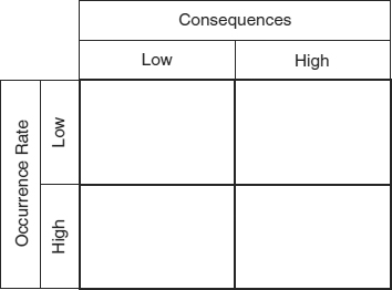
EXHIBIT 62.3 “Jacobson's Window,” A Simple Risk Model

Questionnaires are appealing because they appear to relieve the risk assessor of the need to probe into the business system being assessed, but something better is needed for a valid risk assessment. The remaining sections of this chapter build a model of risk and then show how to apply quantitative parameters to the model. Although a greater effort is required, far superior results are achieved.

62.4 MODEL OF RISK.

Exhibit 62.3 is a simplified model of threats and consequences devised by the author of this chapter. The model takes the first steps toward quantification of risks. In this very simple model, all risk events are assumed to have either a low or high rate of occurrence, and all consequences of risk event impacts are assumed to be either low or high. William H. Murray, at the time an executive consultant at Deloitte and Touché, referred to this risk model as Jacobson's Window. Let us now consider the implications of the model.

62.4.1 Two Inconsequential Risk Classes.

The two-by-two empty matrix model implies that there are four classes of risk: low-low, high-low, low-high, and high-high. Exhibit 62.4 suggests that two of the classes can be ignored. The low-low class can be ignored because these risks do not matter. As an extreme example, it is obvious that a risk event that occurs at about 10,000-year intervals and causes a $1 loss each time can be ignored safely. Experience suggests that the high-high class can be assumed not to exist in the real world. If 50-ton meteorites crashed through the roofs of computer rooms every day, there would be no attempt to use computers. In practice, high-probability, high-loss risks just do not exist. Catastrophic events do occur, but not frequently.

62.4.2 Two Significant Risk Classes.

This analysis suggests that there are only two significant risk classes: high-low and low-high. Data entry keystroke errors are an example of a high-low risk: a high probability of occurring and usually a low resulting loss. A major fire that destroys the building housing an IT system is an example of a low-high risk: a low probability of occurrence and a high consequential loss. However, we know that real-world risks do not fall into just these two classes. Instead there is a spectrum of risks from high-low to low-high.

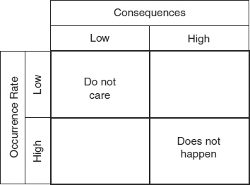
EXHIBIT 62.4 Two Inconsequential Risk Classes

62.4.3 Spectrum of Real-World Risks.

Exhibit 62.5 illustrates the distribution of representative risks from high-low (keystroke errors) to low-high (major fires). Conceptually, there is little difference between the high-low and low-high threats. Experience suggests that averaged over the long term, the high-low and low-high threats will cause losses of similar magnitude to an organization. This concept is quantified by the notion of annualized loss expectancy. The ALE of a risk is simply the product of its rate of occurrence, expressed as occurrences per year, and the loss resulting from a single occurrence expressed in monetary terms, for example, dollars per year.

Here is a simple example of ALE: Assuming that 100 terminal operators each work 2,000 hours per year and make 10 keystroke errors per hour, the occurrence rate of keystroke errors would be 2 million per year. Next, assuming that 99.9 percent of the errors are immediately detected and corrected at an insignificant cost, then 2,000 errors slip by each year, a high occurrence rate risk, and must be corrected later at a cost estimated to be $10 each, a low consequence for each occurrence. Thus, the ALE of the high-low risk: Keystroke error is estimated to be 2,000 occurrences per year × $10 per occurrence, or an ALE of $20,000/year.

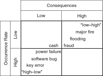
EXHIBIT 62.5 Spectrum of Real-World Risks

Continuing our example, assume that the probability of a major fire in any one year is 1/10,000 (in other words the annualized probability of occurrence of a major fire is estimated to be 0.0001), and if the loss resulting from a major fire would be $200 million, then major fire is a low-high risk. These assumptions lead to an estimate of $20,000/year for the ALE of major fires.

Thus, the two risks from opposite ends of the risk spectrum are seen to have ALEs of about the same magnitude. Of course, we have manipulated the two sets of assumptions to yield similar ALEs, but the results are typical of the real world. However, note that we are assured of having a loss of $20,000 every year from keystroke errors, but a loss of $200 million in only one of the next 10,000 years.

Exhibit 62.6 is a computer-generated⁸ plot of threat occurrence rates and consequences (total single-occurrence loss) taken from an actual quantitative risk analysis of a facility. Each of the numbered boxes represents a threat type. Because the two scales are logarithmic, the contours of constant ALE are diagonal straight lines. As expected there are no threats in the high-high (doesn't happen) and low-low (trivial) zones.

Although the ALEs span a range of about four orders of magnitude, (from about $50 per year to about $500,000 per year), frequencies and consequences each span about seven orders of magnitude. This result is typical of the real world and illustrates the fundamental flaw in high-medium-low risk models like the matrix in Exhibit 62.7. These models attempt to simplify risk assessments by defining a very limited range of values, three each, for frequency and consequence. As a result, threat event ALEs that differ by as much as two orders of magnitude, as illustrated in Exhibit 62.5, are given the same ranking when assessed using a high-medium-low matrix.

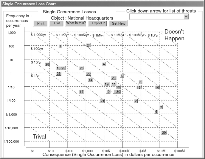
EXHIBIT 62.6 Plot of Actual Threat Frequencies and Consequences Copyright 2005 International Security Technology, Inc.

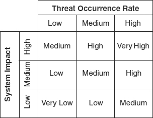
EXHIBIT 62.7 Typical Risk Matrix

Proponents of this risk model are silent about the details. First, as Exhibit 62.6 shows, the “Very High” and “Very Low” risks are meaningless in the real world. Second, the matrix requires users to compress numerical values with a range of almost seven orders of magnitude (e.g., from 100/year to 1/20,000 years) into only three values: Low, Medium, and High. In other words, two risks with same consequence but occurrence rates that differ by a factor of 100 might receive the same evaluation. Likewise, because of the arbitrary boundaries between low, medium, and high, two risks with the same consequence but with occurrence rates that differ by 1 percent could receive different ratings. These considerations defy common sense and make it clear that rating a risk as high, medium, or low cannot be the basis to cost-justify a proposed risk management measure.

62.5 RISK MITIGATION.

Exhibit 62.6 shows that the effect of risk exposures on IT systems can range from trivial to catastrophic, and it is not always immediately obvious which risk exposures are the most dangerous. For this reason, it is essential to base the selection of risk mitigation measures on a quantitative assessment of risks. In this section, we consider the practical considerations in generating quantitative assessments and applying them to risk mitigation decisions.

62.5.1 ALE Estimates Alone Are Insufficient.

As noted, ALE is a useful concept for comparing risks, but we recognize intuitively that ALE alone is not a sufficient basis for making risk mitigation decisions about the low-probability high-consequence risks. There are two reasons for this.

1. The difficulty in generating a credible estimate of occurrence rate for low-probability risks. As a rule, one can generate credible estimates of the consequences of a low-probability risk, but the same is not true of its occurrence rate. Risks that flow from human actions such as fraud, theft, and sabotage are also difficult to quantify credibly.
2. A common human trait that this writer has postulated as Jacobson's 30-Year Law:

Why 30 years? It is not clear, but it may be related genetically to human life expectancy, which until just a few generations ago was about 30 years. Possibly people who were able to suppress anxiety about rare events were more successful than those who worried too much. Numerous instances of Jacobson's 30-Year Law can be found. For example, the U.S. Government has had a major fire at about 28-year intervals beginning in 1790, most recently at the Military Records Center. Presumably, each new generation of federal property managers must relearn the lessons of fire safety by direct experience. The Northeast power blackout of 2003 followed a similar event in 1976, 27 years earlier.

It seems to be common for senior managers, particularly public officials, responding to a calamity (e.g., Hurricane Katrina), to say something like this: “Who could have imagined that such a thing would happen? However, we have taken steps to see that it will never happen again.” This is an imprudent statement for two reasons. First, prudent managers will anticipate potential disasters. Second, saying “never” implies that perfect security is the goal. This is nonsensical since perfect security is infinitely expensive and so cannot be achieved.

62.5.2 What a Wise Risk Manager Tries to Do.

Unlike the senior managers just quoted, an organization's risk manager should be trying to imagine every possible material risk the organization faces, even those not personally experienced, and developing estimates of the impact of these risks. Next, the risk manager should strive to identify the optimum response to each material risk by identifying security measures that have a positive ROI. Potentially fatal low-occurrence/high-consequence threats require treatment irrespective of ALE and ROI as discussed in Section 62.5.4.

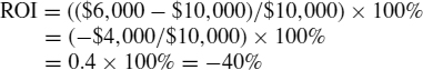
Consider this example of cost-effectiveness: The ALE for keystroke errors was estimated in the Section 62.4.3 example as $20,000 per year, or $200 per operator. This estimate is credible because presumably there has been ample past experience with both the occurrence rate and impact cost of the keystroke-error risk. The risk manager considers how to treat this risk. Imagine that experience suggests that spending $100 each year on keyboard skills training for each operator would reduce the undetected error rate by 30 percent. Because the $100 per operator expense would yield a benefit of $60 in reduced ALE (30 percent of $200, the per-operator ALE), the ROI⁹ of training would be −40 percent, clearly not a cost-beneficial mitigation measure. In effect, we would be spending $10,000 to achieve a $6,000 loss reduction. However, if the error rate were reduced by 90 percent instead of 30 percent, the training would appear to be a good investment; spending $100 each to train operators, would produce a reduction in ALE per operator of $180, an ROI of +80 percent. The goal of the risk manager is to find the package of risk management measures that yields the greatest overall ROI.

62.5.2.1 Three Risk Management Regions.

Basing risk management decisions on ROI estimates, as described, does not work for the low-probability, high-consequence risks because of two negative factors: (1) the credibility of risk estimates and (2) management's concern about the risk consequences. End users commonly have a higher level of concern about risks than IT system managers, but as a rule it is the IT system managers who make the decisions about security measures. An IT system manager generally has no difficulty choosing between buying a faster server and a more reliable server. The benefit of higher throughput is immediately evident. The benefit of higher reliability is not as obvious. Thus, although a risk manager may identify a significant low-occurrence, high-cost risk before it has occurred, an organization's senior managers probably would be unaware of these low-high risks and would be genuinely surprised were a major loss to occur. Hence, the “Who could have imagined…” press releases. In other words, simply identifying an exposure might be thought to be enough to justify adoption of a mitigation measure to address the exposure. This suggests that the risk manager needs additional criteria for selecting risk mitigation measures. The next section presents an overview of mitigation measures to clarify the selection criteria.

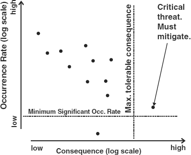
EXHIBIT 62.8 Three Risk Zones

Copyright 2002 International Security Technology, Inc.

It will help risk managers to understand that the universe of risk events to which an organization is exposed by dividing the total risk space into the three regions shown in Exhibit 62.8. The two axes are logarithmic, and the dots represent individual threats.

These regions help define appropriate risk management actions. The boundaries of the regions are defined by two senior management decisions.

1. The first decision is to define the minimum significant threat event occurrence rate. The concept is that it is reasonable to simply ignore the risk of threat events for which we have estimated occurrence rates less than some minimum rate. For example, senior management may decide to ignore risks with occurrence rates estimated to be less than once in 20,000 years (i.e., the probability of an occurrence of the threat next year is estimated to be less than 0.00005).
2. Senior management may also identify a loss level (consequence) that is intolerably high. Risk events of this type will appear in the lower right of Exhibit 62.6, and 62.8. The occurrence rate of these events is immaterial as long as they exceed the minimum consequence criterion and the minimum occurrence rate. If we estimate that the loss caused by an occurrence of a threat event (commonly referred to as the single-occurrence loss [SOL]) exceeds the loss threshold and the occurrence rate exceeds the minimum material occurrence rate, then we must take steps to reduce the loss, perhaps by transferring the risk with an insurance policy or by reducing the estimated occurrence rate to a value below the minimum material occurrence rate.

It is instructive to consider where to plot an unusual risk event like the attack on the World Trade Center (WTC) on September 11, 2001. It is likely that many organizations have facilities that would generate losses in excess of their maximum tolerable loss if totally destroyed by a similar terrorist attack. This implies that such organizations should take steps to protect these facilities against terrorist attacks. However, we should also take into account the estimated rate of occurrence before making a decision. How can we make a credible estimate of such a rare event? We can begin by estimating how many such events will occur next year in the United States. For example, based on past experience, we might assume that there will be about two such attacks each year. Then we estimate the likelihood that, of all the facilities in the United States, our facility would be selected for attack. This will depend on the “attractiveness” of our facility to a terrorist group when compared with all other potential targets in the United States. For example, assume that there are 100 “attractive” buildings that are as widely recognized and as vulnerable as the WTC. If our facility is one of the 100, then we might estimate the occurrence rate as 1/100 × 2, or a probable occurrence rate of 0.02/year. If, however, our building is not one of the 100 high-profile buildings, then we might estimate that if there are 200,000 similar buildings in the United States, our occurrence rate is 1/200,000 × 2, or an occurrence rate of 1/100,000 years. In this latter case, our senior management probably would choose to ignore the risk.

The remaining portion of the Exhibit 62.6 graph, the mid- to upper-left-hand corner, is the zone where the risk manager attempts to find cost-beneficial risk management measures, as discussed in the next sections.

62.5.2.2 Where ROI-Based Risk Management Is Effective.

ROI-based mitigation works well for high-probability, low-consequence risk exposures for two reasons: The manager who approves the expenditure (1) believes that the risk exists and should be addressed and (2) believes further that the parameters used to generate estimates of ALE and the reduction in ALE, used to estimate ROI, are reasonable and credible.

62.5.2.3 Four Reasons for Adopting a Risk Management Measure.

There are four general tests of the utility of a risk management measure.

1. The measure is required by law or regulation. In effect, a governing body has determined (one hopes) that the measure makes good public policy because it will always meet one of the remaining three tests. Exit door signs in public buildings are a good example. Sarbanes-Oxley may be an example of a bad (not cost-effective) law.
2. The cost of the measure is trivial but its benefit is material. For example, a little-used door that compromises physical access controls is not being kept locked. One can institute a procedure and install security hardware to keep the door locked at very low cost.
3. The measure addresses a low-high risk that has an intolerable single-occurrence loss, as discussed in Section 62.5.2.1. For example, it would be intolerable for a corporation to experience an SOL that exceeded owner equity or net worth. The failure several years ago of a prominent British merchant bank following unwise speculation by a staff member is a tragic example of an organization that failed to identify and address an intolerable SOL exposure.
4. The cost of the measure will be more than offset by the reduction in future losses (ALE) that it will yield. In other words, the mitigation measure has a positive ROI. This reason is commonly used to justify protection against the high-low risks. Operator keyboard training described in Section 62.5.2 is an example.

Procedures for managing the last two risk categories follow.

62.5.3 How to Mitigate Infrequent Risks.

After the high-low threats have been addressed using an ROI analysis, the risk manager considers all imaginable low-high risks, one by one, and makes for each such risk an estimate of the SOL and the rate of occurrence. The report of this analysis should describe for each threat the confidence level of the estimates of its SOL and occurrence rate. These estimates are arranged in descending order of SOL. The list is presented to senior management, who draws a line somewhere on the list and says, “The risks above the line are intolerably high. Do something about them.” The risk manager then considers each of the unacceptable risks in two ways.

62.5.3.1 Reduce the Magnitude of High Single-Occurrence Losses.

Sometimes the magnitude of an SOL can be reduced. There are several possibilities:

• Transfer the risk by obtaining insurance against it. The premium will depend in part on the amount of the loss that is deductible. For example, one might obtain insurance against a $100 million SOL with a $10 million deductible to minimize the insurance premium. In effect, the intolerable $100 million SOL has been reduced to a tolerable $10 million SOL at the cost of the insurance policy premium.
• Disburse the risk exposure. For example, replace a single IT center with an intolerable SOL of $500 million of catastrophic physical damage, and service interruption losses, with three centers having SOLs of about $167 million each. The centers should be sufficiently isolated from one another to rule out shared disasters. The cost will be the incremental cost of the less efficient operation of three facilities.
• Reduce the vulnerability of the IT system to the risk. For example, implementing an enhanced business resumption plan, at some additional cost, can speed up recovery off site. This will reduce the SOL associated with catastrophic service interruption losses. Notice that this an example of a risk mitigation measure that affects more than one threat.

The risk manager also may strive to reduce the occurrence rate of a high SOL. Because of the uncertainty of the estimates of low occurrence rates, this is less satisfactory. Nonetheless, even the uncertain occurrence rate estimates can be useful. If two risk exposures have the same SOL but differ by an order of magnitude in estimated occurrence rate, it is reasonable to assume that the risk with the lower occurrence rate represents a lesser danger to the organization.

62.5.3.2 Risk Management Measures Selection Process.

Assume that the risk manager has presented a risk assessment/risk mitigation report to senior management as described. The report lists the low-high risks with one or more strategies for treating each risk.¹⁰ The senior manager is responsible for selecting the mitigation measures for implementation because, as noted, ROI-based justification is inappropriate for this class of risks.

1. If the risk manager is able to identify a relatively low-cost mitigation measure that reduces the rate of occurrence of a risk to a low enough value, senior management may elect to adopt the mitigation measure.
2. There is some rate of occurrence below which the senior manager is willing to ignore a risk, even if the estimate is low confidence. Typically this applies to very low occurrence rate events. Extreme examples are a nuclear detonation or a crashing meteorite.
3. Risk transfer by insurance, or one of the other techniques listed earlier, reduces the SOL to a tolerable level, and the senior manager is willing to accept the cost of the insurance coverage.

A complete tabulation of occurrence rates and the costs of mitigating actions for all the high-SOL risk exposures will help senior management to prioritize the implementation of the mitigation measures.

62.5.4 ROI-Based Selection Process.

After the potentially fatal risks have been addressed as described, the risk manager can turn to selection of measures to address the remaining high-low risks. A five-step procedure for selecting strategies on the basis of ROI is straightforward.

1. For each of the threats, identify possible risk management measures. As noted, some measures will affect more than one threat. There are four possible strategies:
   1. Threat mitigation. Measures to reduce the occurrence rate and/or the impact of one or more of the threats.
   2. Risk transfer. Use an insurance policy or other contractual means to transfer some or all of the risk to another party.
   3. Business resumption plans. Take steps in advance of threat occurrences to decrease the time required to resume business operations. This type of strategy applies to non-IT business systems that are included in the scope of the risk management project.
   4. IT system recovery plans. Take steps in advance of threat occurrences to decrease the time required to resume operation of the IT system and to reduce the amount of stored data lost. (See Section 62.6.3.3 for details.)
2. For each strategy, estimate the present value of the cost to implement and maintain the measure, taking into account the remaining life of the facility, the useful life of the measure, and the applicable time value of money. The organization will not enjoy the full benefit of a measure with a high initial cost and a low annual support cost if the life of the facility is less than the life of the measure.
3. For each strategy, estimate the effect of the measure on the occurrence rate and consequence of the threat(s) that the strategy addresses. Use these data to calculate total ALE assuming the measure is implemented. Calculate the present value of the reduction in total ALE the strategy is expected to yield. This is the benefit of the measure. Note also that in addition to reducing risks, a strategy may reduce operational costs. This cost saving should be added to the ongoing benefit (ALE reduction) of the strategy.
4. Using the values of cost and benefit, calculate ROI:

   ROI = (($Benefit − $Cost)/$Cost) × 100%

   For example, using the data in Section 62.5.2, ROI is calculated as:

   

   This equation normalizes the ROI and expresses it as a percentage. Zero percent represents a neutral ROI (benefit equals cost). One hundred percent would represent a very beneficial measure, and 1,000 percent would probably be a no-brainer. If the measure generates a cost saving, the saving is added to the ALE reduction benefit when calculating the ROI. Note that the ROI analysis of a risk mitigation measure will understate its benefit if the risk assessment does not include all the risk events that the measure will address.

5. Make a list of the strategies in descending order of ROI after discarding the strategies with a negative ROI.

Presumably, management now selects for implementation the strategies in descending order of ROI until all available resources are allocated. However, if two or more strategies impact the same threat, it is possible that their effects may be partially overlapping. The risk manager can investigate this possibility in this way. Begin by assuming that the most attractive strategy has been implemented and recalculate the “baseline ALE.” Next, verify the parameters for the remaining strategies, taking into account the effect of the measures assumed to have been implemented. Recalculate their ROIs as described, and repeat the selection process. It would be convenient if there were an analytic way to do this, but this author has been unable to devise a practical way to do so because of the wide range and complexity of potential interactions.

62.5.5 Risk Assessment/Risk Management Summary.

The risk model illustrated by Jacobson's Window leads to five conclusions.

1. Risks can be broadly classified as ranging from high-probability, low-consequence to low-probability, high-consequence events. In general, risk events in this range cause losses over a relatively narrow range of loss values when expressed as an annual rate or ALE.
2. Because of IT operating staff familiarity with the high end of the high-low risks, all available measures may already have been taken such that there may not be any cost-beneficial way to further reduce the ALE of some of these threats.
3. Midrange risks can be addressed by selecting mitigation measures with a positive ROI, based on the relationship between the cost to implement a mitigation measure and the reduction in ALE it is expected to yield.
4. Treatment of low-high risks requires the judgment of senior management, based on estimates of SOL and, to a lesser extent, estimates of rate of occurrence. Mitigation measures or risk transfer may reduce single-occurrence losses to acceptable levels or decrease occurrence rates to the level at which risks can be ignored.
5. To be effective, the risk management function must be:
   • Performed by properly qualified persons.
   • Independent of IT line management.
   • Reported to senior management to ensure that all risks are recognized and that resource allocation is unbiased.

62.6 RISK ASSESSMENT TECHNIQUES.

The first step in performing a risk assessment is to define the scope and focus of the assessment. The scope will define the IT functions or business processes, the physical assets, the intangible assets, and the liability exposures that are to be included in the assessment. The focus means the kinds of risk events to be included in the analysis. Risk events may include failures of the IT hardware and software, software logical errors, deliberate destructive acts by both insiders and outsiders, and external events such as earthquakes, hurricanes, river floods, and so forth. Sometimes the focus is determined by the desire to evaluate a specific class of risk management measures.

62.6.1 Aggregating Threats and Loss Potentials.

Aggregation is a key concept of quantitative modeling, and refers to the practice of combining related items to keep the model at a manageable size. For example, one can define a single risk event (IT server failure) or two risk events (Server01 failure and Server02 failure) under the assumption that the two servers support different systems with different loss potentials), and so on in ever-increasing detail. The more risk events defined for a risk assessment, the greater will be the effort required to establish the risk parameters and perform the calculations. However, the individual risk events will not all have the same impact on the results of the assessment. Indeed, some risk events will be found to be completely inconsequential, so the time expended to estimate their parameters will have been wasted. In other words, an appropriate degree of detail will not be immediately obvious.

This suggests that one should begin an assessment using highly aggregated risks, functions (typically business processes), and assets, perhaps no more than 10 to 15 of each in a typical situation, together with roughly prepared estimates of the risk parameters. This preliminary analysis will show which elements are important to the results. One can then add details to the important elements as appropriate and refine the material estimates to improve the validity of the model. This approach works to concentrate the effort on the important issues and avoids wasting time refining unimportant input data.

62.6.2 Basic Risk Assessment Algorithms.

It is generally accepted that ALE, in dollars (or other currency as appropriate) per year, is calculated as:

The term “threat occurrence rate” (TOR) is used to designate the estimate of the probability of occurrence of a threat event during a risk management planning period, typically one year. Thus the TOR is the probability of occurrence at an annualized rate. The functions and assets are characterized by their potential to trigger a loss when impacted by one or more of the threats. The term “potential for loss” or simply “loss potential” is used specifically to designate the worst-case loss a function or asset can generate. This implies that there is at least one threat event (the worst-case threat) that will trigger a loss equal to the loss potential. Other threats will cause lesser losses because they have a lesser effect on the function or asset. The threat effect factor is used to quantify the relationship between a threat event and a function or asset. If the threat event has no impact on the function or asset, the corresponding threat effect factor will be zero. If the threat event triggers the worst-case loss (the loss potential), the threat effect factor will be 1.0. Threat effect factors will range from zero to 1.0 for all threats.

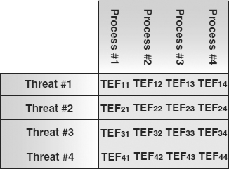
EXHIBIT 62.9 Threat Effect Factors Connect Threats and Processes, Functions, and Assets

Exhibit 62.9 illustrates how each threat-function or threat-asset pair includes a threat effect factor. The single-occurrence loss, expressed in monetary units for each function or asset with respect to a given threat event, is calculated as:

The terms “loss potential” and “threat effect factor” are as defined. The sum of the SOLs for all the functions and assets with respect to a given threat is the consequence of an occurrence of the threat.

From these two definitions, we can see that:

The sections that follow discuss these two equations in more detail and describe techniques for estimating values for TOR, loss potential, and threat effect factor.

62.6.3 Loss Potential.

There are four basic kinds of losses that contribute loss potential:

1. Property damage losses. Property damage losses occur when a threat event impacts an asset of the organization. The asset may be physical property damaged, for example, by a fire or flood, or the asset may be an intangible asset, such as a trade secret or a proprietary database, the improper disclosure, modification, or destruction of which causes a loss to the organization.
2. Liability losses. The operation of an IT system may expose the organization to liability for damage or injury. For example, improper operation of an IT-controlled process might release a toxic gas. Improper disclosure of personal information may cause the individual to sue the organization for damages. If third parties place reliance on data generated or maintained by an IT system, there may be an exposure to damage suits if the data are incorrect as a result, for example, of flaws in the IT system.
3. Service interruption losses. Service interruption losses occur when IT system services or other business functions are interrupted or are not initiated in a timely manner because of the action of a threat event. In general, the longer the duration of an interruption, the greater will be the amount of the loss. This means that service interruption loss potential must be estimated in the form of a table of values appropriate to the expected range of interruption durations the threats are expected to generate. As a consequence, each threat that causes service interruptions must be defined in terms of the percentage of the threat's occurrences that result in each of the interruption durations used to define service interruption loss potential.
4. Lost data losses. IT systems typically require stored data to function. If the primary copy of the stored data is lost, the data are recovered from the most recent backup copy or reconstructed from paper records, if they exist, of prior transactions. The magnitude of the data loss will depend on the rate at which the stored data change, the frequency with which a backup copy is made, the accuracy of the backup copy process, and the frequency of the occurrences of the threat events that require data recovery of the stored data. The stored data used by some IT systems do not change continuously, and so a complete backup copy can be made after each update phase, and data loss thus avoided.

Loss potentials, as described in the next three subsections, are based on estimates of the worst-case losses with respect to the list of risk events.

62.6.3.1 Property and Liability Losses.

Property and liability losses are treated the same way, so they can be discussed together. It is advisable to begin consideration of property damage losses by making an aggregated list of possible sources. For example, the initial list might consider together all the hardware in an IT facility and all of the databases needed to operate each of the principal IT applications. For each such asset,¹¹ an estimate is made of the worst-case loss that the organization could experience with respect to that asset. For example, the worst-case loss for a set of stored data would be the cost to reconstruct the data from backup copies and the cost to recover any missing or corrupted data. There will be other losses resulting from interruptions to IT services that require the availability of the data, but these losses are described separately in the next subsection.

Liability¹² loss potentials, if included in the scope of the risk management project, should be estimated in the same way. The first step is to determine which liabilities should be included in the risk assessment. The organization may already have a mechanism for addressing liability exposure, possibly through a risk transfer mechanism. However, the liability exposures that are unique to the IT operations should be included and the worst-case loss potential estimated as described.

62.6.3.2 Service Interruption Losses.

Service interruption (sometimes referred to as denial of service¹³) losses refer to the losses experienced by end users of an IT system when the service is not performed on time. The first step in estimating service interruption losses is to construct a list of the IT services for which there is a significant interruption loss potential. Here, too, it is desirable to aggregate individual applications in basic service areas. Examination of a wide range of functions suggests that there are six different classes of service interruption losses. Since each class of loss may begin after a different interruption duration, it is unlikely that there will be a single loss rate that begins at the instant the interruption begins and has a fixed rate per hour of interruption duration into the indefinite future. Reviewing the causes with the persons most familiar with each service, typically the line-of-business managers, will determine which classes apply and what the loss potential factors are. By tabulating the losses associated with each of the classes, one can generate an overall loss potential for a suitable range of service interruption durations.

1. Reduced productivity. Would people be idled if there were a service interruption? If yes, how many and how soon? What, approximately, is their total pay, including benefits? If substantial production facilities would be idled, what is the approximate hourly cost of ownership of the facilities, computed as the total life-cycle cost of ownership divided by the total operating life in hours?
2. Delayed collection of funds. Does the IT system application trigger collection of funds for the organization (e.g., a billing system or a loan-notes-due collection system)? If yes, determine the average amount collected each business day that would be affected by a service interruption. Because in most cases it will be possible to do some manual processing of the high-value items, the affected amount may be less than the full daily processing dollar volume. Determine a suitable cost-of-money percentage for use in present-value calculations by consulting the organization's treasurer or controller. Alternatively, the current commercial bank prime rate plus one or two percentage points can be used. The total loss does not increase linearly with the duration of the interruption. For example, assume that the one-day loss is $100 due to delayed collection. After a two-day outage, the loss would be $300: $200 from the first day and $100 from the second day. A three-day outage would cost $600: $300 of accumulated losses for the first day, $200 for the second day of delayed collections, and $100 for the third day, and so on.
3. Reduced income. Will an interruption of the application impact sales revenue or other income receipts? If yes, estimate the amount of income lost both immediately, and over the long term, for a range of service interruption durations appropriate to the risk events included in the risk assessment. It may be difficult for the end user to make an estimate, unless it is possible to remember the last major service interruption and to describe what happened. What would the organization do if a major competitor had a service outage? How would the outage become known, and how would it be exploited to increase income? These questions may help to determine the amount of reduced income to be expected.

   Along with reduced income, there would probably be a reduction in operating expenses, such as cost of sales, caused by the decreased activity. When the reduction in operating costs is subtracted from the reduced revenues, the result is the net loss. Estimates should be made for the shortest service interruption duration that the user believes would cause significant lost business; in addition, planning should include provisions for one or more service interruptions of greater duration.

4. Extra expense. How would the user respond to an outage? Would it be necessary to hire temporary help or to work overtime? Could an outside service be used? Would there be an increased error rate, which would increase error research and correction expenses? Might there be increased fraud loss and fraud investigation costs? The cost to catch up, after the outage ends, is often a major extra expense factor. Beginning with the shortest significant duration, several estimates should be made, including a worst-case scenario.
5. Lateness penalties. If the application entails any lateness penalties, contractual, regulatory, or legal, an estimate should be made of the amount of the penalties that would be triggered by an outage, and the outage duration that would trigger the penalties.
6. Public perception. Public perception, as a catchall term, refers to the indirect effects of a service interruption. Staff morale and customer attitudes may be affected negatively by the impression that the organization's risks are not being effectively managed. The value of publicly traded stock may be adversely affected, and pending mergers or stock offerings may be derailed. The cost of borrowing may increase.

This procedure does not involve asking end users to estimate the maximum “tolerable” service interruption duration. This is not a useful question. An attempt by end users to establish the value of tolerable is simply an opinion or subjective judgment call. The basic risk assessment will establish the expected annualized losses. Then an evaluation of the cost-benefit or ROI of alternative risk mitigation measures, implemented to reduce the number and duration of service interruptions, will identify the optimum IT system configuration, including measures to control service interruptions.

62.6.3.3 IT Systems Interruption Mitigation.

IT system service interruption mitigation is a special case because of the effect of lost-data losses. This is why.

The performance of IT system continuity plans is often characterized using two parameters referred to as recovery time objective¹⁴ (RTO) and recovery point objective (RPO). RTO is the maximum service interruption duration that will result from the action of threats on an IT system. The RTO of the continuity plan in place for an IT system will determine the expected losses of an IT system that result from the impact of the service interruption threats. Decreasing the RTO will decrease the expected loss but will increase the cost to implement and maintain the IT system continuity plan.

The RPO is a measure of the frequency with which an IT system backs up stored data. The more frequently data are backed up, the lower will be the lost data losses but the greater will be the cost to install and maintain the backup provisions.

The risk management task is to pick the IT system continuity plan (RTO-RPO combination) that has the most favorable cost benefit. The cost is the cost to install and maintain a given RTO-RPO combination. The benefit is the reduction in expected loss the RTO-RPO combination will achieve, compared with the RTO-RPO combination currently in use. This is why the question “What is your maximum ‘tolerable’ outage duration (i.e., RTO)?” is worthless. A rational selection depends on both cost and benefit, not the subjective appeal of any particular RTO.

Typically, there is an interaction between RTO and RPO. For example, tape is probably less expensive as a backup storage medium than disk, so we would expect a tape-based IT system continuity plan to be cheaper than a disk-based plan. However, tape will restrict the range of RPOs that can be implemented and may control the best achievable RTO, both of which will increase expected loss. There is another important point: There is no inherent connection between the service interruption loss potential of an IT system and the cost of RTO-RPO combinations for the system.

For example, a small inexpensive system (one with low RTO and RPO costs) might be running a very time-critical, high-value function (e.g., currency trading), while a large system with high RTO and RPO costs might be analyzing the works of William Shakespeare for the local college, a low-criticality task.

62.6.4 Risk Event Parameters.

As noted in the prior section, during the determination of loss potential, a list of significant risk events can be constructed. The list should be examined critically to determine if additional event types should be added to it, bearing in mind the aggregation considerations discussed earlier and the defined scope of the project.

Once the risk events list has been completed, two parameters are estimated for each event:

1. Occurrence rate. There are several ways to estimate occurrence rates. If the event has had a relatively high occurrence rate in the past, typically more than once in 10 years, the organization is likely to have records of those events, from which the occurrence rate can be inferred with high confidence. However, there are two cautions.
   1. Consideration must be given to any changes in the environment that would affect the occurrence rate. For example, the root cause of some system crashes may have been corrected, so that one would expect the future rate to be lower than in the past.
   2. It is important to avoid double counting. For example, a system outage log may lump electric power failures into a catchall category: hardware failure. If electric power failure is included in the risk assessment as a separate risk event, its occurrences may be inadvertently counted twice.

      If the risk event is external to the IT facility—for example, river flooding and earthquake—one can usually find external sources of information about past occurrences. For example, one could use the Web page www.nhc.noaa.gov/pastint.html to determine if a given U.S. location has ever been impacted by a high-intensity hurricane. Numerous Web sites can support a risk assessment. One also may find that past copies of local publications can help to determine the past local history. In some cases, there will be no meaningful past history for a risk event, particularly if the event is of recent origin, such as e-business fraud and terrorism. In these cases, it may be possible to reason by analogy with other similar risk events to develop a reasonable estimate.

2. Outage duration. The range of outage durations for each threat must be estimated in order to be able to estimate service interruption losses. If the outage duration is not the same for all the IT systems that the risk event impacts, one may either use an average value or define a separate risk event for each of the systems, keeping in mind the aggregation considerations just discussed.

Until an initial overall risk assessment, such as Exhibit 62.6, has been generated, analysts do not know which of the input data are important. Consequently, it is counterproductive to devote effort to refining initial data. The wide range of values encountered in a typical risk assessment makes it clear that rough initial estimates of the risk parameters will be sufficiently accurate to identify the critical parameters.

62.6.5 Threat Effect Factors, ALE, and SOL Estimates.

From the basic risk assessment algorithms, it is possible to determine the risk event/loss potential pairs for which the threat effect factor is greater than zero (see Section 62.6.2), and having done so, to estimate the value of the factor. It is then possible to use the risk data discussed earlier and the algorithms to calculate an estimate of the ALE and SOL for each of the pairs, and then to tabulate the individual ALE and SOL estimates to obtain a complete risk assessment for the IT organization. This is useful as a baseline because it provides an assessment against which to evaluate potential risk mitigation measures. In other words, the benefit of a risk management measure is the amount by which it reduces this baseline or current expected loss estimate.

In order to validate the assessment, it is necessary to identify the threat event/loss potential pairs that account for the majority of the expected losses. Typically, about 20 percent of the pairs cause 80 percent of the total expected loss. Reviewing the details of each input item, these questions should be asked: Were source data transcribed correctly? Are the assumptions reasonable? Were calculations made correctly? Does any threat event/loss potential pair account for so much of the expected losses that it should be disaggregated from other data items? Once the validation process is complete and indicated changes have been made, it is feasible to consider risk mitigation, but first one must gain acceptance of these data.

Field experience has disclosed a very powerful technique for gaining acceptance of estimates used in the risk assessment. First we gather data from knowledgeable people in the organization: line-of-business managers, IT specialists, audit, security, and the like. We use these data to make a preliminary baseline estimate of risks as described. We then convene a round table meeting of all the people who provided the data. We show them the results and the input data. This results in a useful discussion of the data and tends to identify inputs based on faulty assumptions, personal biases, and misinformation. It is rather like an instant peer review. The agreed changes to the input data are then used to make a final estimate of risks, which can be used to evaluate proposed mitigation measures.

62.6.6 Sensitivity Testing.

The preceding discussion implies that a single value is to be estimated for each of the risk parameters included in the risk assessment. However, it may be thought that a parameter should not be limited to a single value and that a Monte Carlo technique should be used to generate a set of ALE and SOL estimates. In a Monte Carlo approach, one generates random inputs into a model following specified probability distribution functions for each of the variables being studied. The outputs of the model then generate frequency distributions that allow one to evaluate the sensitivity of critical outputs to the precision of specific inputs. There are two obstacles to using this approach. Apart from the big increase in the complexity of the calculations, there is still a requirement to select a single risk mitigation strategy based on the set of ALE and SOL estimates. It is not feasible to install a range of performance value for a given mitigation measure to match a range of loss estimates. As described previously, cost-beneficial risk mitigation measures are selected by calculating the baseline ALE and then recalculating the ALE, assuming that the proposed mitigation measure has been installed. The difference between the two ALE estimates is taken to be a reasonable estimate of the return in the ROI calculation. Assuming two sets of 1,000 ALE estimates (without and with a proposed mitigation measure) generated by a Monte Carlo simulation, calculating all possible differences produces a set of 1 million returns. Which one should be selected to calculate ROI?

Using the most likely value for each risk parameter and generating only two ALE estimates, the difference between the two may be used to calculate ROI. Because the ROI typically flows from a relatively large number of parameters, the overall result will tend to average out any individual departures from the average values used, and so will be a fair representation of the actual risk losses that will occur.

However, if confidence in the accuracy of an estimate is extremely low, estimates using low, median, and high values of the parameters should be used to evaluate the effect on the overall results. Whenever a risk assessment includes a material low-confidence parameter, full disclosure should be made to the managers who review and act on the results. Risk analysts should bear in mind that almost all other decisions about resource allocations that senior managers are regularly called on to make are based on uncertain estimates of future events. There is nothing unique about the uncertainties surrounding risk mitigation decisions.

62.6.7 Selecting Risk Mitigation Measures.

The objective of the risk mitigation process is to identify the optimum set of mitigation measures. The first step is to address the intolerable SOL exposures as discussed in Section 62.5.3. The risk assessment and the evaluation of potential risk mitigation measures provide the raw material on which to base an implementation strategy for the risk exposures in the midrange. Considerations include:

1. The mitigation measures with negative ROIs can be discarded.
2. The remaining mitigation measures can be tabulated in three ways:
   1. In descending order of net benefit: ALE reduction minus the implementation cost.
   2. In ascending order of implementation cost.
   3. In descending order of ROI.
3. Based on other considerations, senior management selects mitigation measures from one of the three lists. Two other considerations include:
   1. The availability of resources for risk mitigation may be limited, in which case some mitigation actions must be deferred until the next budgeting period. In extreme cases the lowest-cost measures may be selected.
   2. The mitigation of risk exposures that have a particularly undesirable effect on marketing considerations, as compared with other loss categories, may be given priority.

62.7 SUMMARY.

This chapter has shown the tremendous advantage of having a detailed, quantitative assessment of the risk exposures leading to a quantitative evaluation of prospective mitigation measures. Senior managers will appreciate the advantage of using rational business judgment in place of seat-of-the-pants guesswork.

62.8 FURTHER READING

Berg, A., and S. Smedshammer. Cost of Risk—A Performance Vehicle for the Risk Manager. Linköpings, Sweden: Linköpings University, 1994.

Gordon, L. A. Managerial Accounting—Concepts and Empirical Evidence. McGraw-Hill, 2000.

Hamilton, G. This Is Risk Management. Studentlitteratur: Chartwell-Bratt, 1988.

Jacobson, R.V. “Operational Risk Management: Theory and Practice.” Symposium of Risk Management and Cyber-Informatics, Orlando, FL, 2004.

Jacobson, R. V. “What Is a Rational Goal for Security?” Security Management (December 2000).

Lalley, E.d P. Corporate Uncertainty & Risk Management, Risk Management Society Publishing, 1982.

Murray, W. H. “Security Should Pay: It Should Not Cost.” In: Proceedings of the IFIP/Sec '95. Chapman & Hall, 1995.

National Institute of Standards and Technology. Guideline for the Analysis of Local Area Network Security. Federal IT Standard Publication 191 (November 1994).

Reiss, R. D., and M. Thomas. Statistical Analysis of Extreme Values, Birkhäuser Verlag, 2001.

Ropeik, D. Risk—A Practical Guide for Deciding What's Really Safe and What's Really Dangerous in the World Around You. Houghton Mifflin, 2002.

Sunstein, C. R. Risk and Reason. Cambridge University Press, 2002.

62.9 NOTES