
The minimum lift-induced drag is generated when the HT generates no (or negligible) balancing force. This happens when the weight is precisely at the aerodynamic center. In that case, the lift-induced drag (using the simplified drag model) is given by:
![]() (ii)
(ii)
On the other hand, when balancing force is required, Equation (i) can be used to calculate the higher lift-induced drag, i.e.:
![]() (iii)
(iii)
The trim drag is the difference between Equations (iii) and (ii):
![]()
QED
Trim Drag of a Wing-Horizontal Tail-Thrustline Combination
Accounting for a high or low thrustline, and wing pitching moment improves the accuracy of the method and is particularly important for long-range aircraft with the thrustline far above or below the CG (see Figure 15-43). Additionally, it is reasonable to account for the wing pitching moment and a possible reduction through the use of a cruise flap. Taking both of these into account yields the following expression to estimate the trim drag:
![]() (15-81)
(15-81)
where
CmW = wing pitching moment coefficient
zT = distance between the CG and the thrustline. It is positive if the thrustline is above the CG
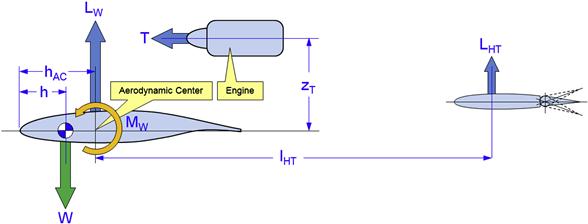
FIGURE 15-43 A simple free-body diagram used to derive trim drag for a wing-HT-thrustline combination.
Comparing Equation (15-81) to (15-80) shows that the wing pitching moment (whose value is <0) and high thrustline (zHT > 0) lead to a higher trim drag.
Derivation of Equation (15-81)
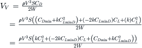
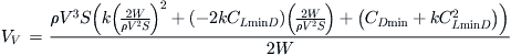
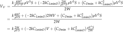
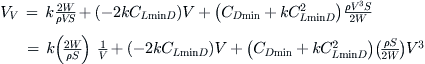
Referring to Figure 15-42, statics requires the following to hold in steady level flight:

These can be solved for the balancing force the HT must generate:
![]()
Inserting this result into the force equation and, as before, using the relation LW = qSCLW, CLW can be determined:
Using the same logic as in the previous derivation, the trim drag can be found to equal:
![]()
QED
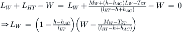
EXAMPLE 15-7
Estimate the trim drag coefficient and drag force for the SR22 at S-L and 185 KTAS assuming the following parameters:
Solution
![]()
![]()
Determine trim drag in accordance with Equation (15-81). For simplicity, rewrite the equation as shown below:
![]()
Where:
![]()
![]()
![]()
Therefore, the trim drag coefficient is:
![]()
This is just about 1.4% to 1.8% of the airplane’s minimum drag coefficient, shown to be 0.02541 in Example 15-18. Using, ![]() , the drag is found to equal 7.7 and 6.0 lbf, respectively.
, the drag is found to equal 7.7 and 6.0 lbf, respectively.
15.5.3 Cooling Drag
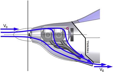
The operation of powered aircraft calls for heat transfer using heat exchangers that are exposed to the free stream airflow. Examples of such heat exchangers are the cylinder head fins of a piston engine as well as radiators for oil and water cooling. An important element of the exchange of energy is the restriction to air flow demanded by the radiator. The flow entering the radiator has a given total head of which some is lost as the air flows through it. This results in a drop in the total pressure of the flow, extracting energy from it. Some of this loss in energy is made up by adding heat to the flow. However, if the heat energy added is less than the energy lost due to the pressure drop, the momentum flux will be reduced. This reduction is experienced as a drag force and is referred to as cooling drag.
Cooling drag is hard to estimate due to the complexity of the flow field inside the engine compartment (see idealization in Figure 15-44). Typically, this is estimated using empirical methods based on testing performed by the engine manufacturer. The following method for estimating cooling drag is an example of such a methodology; here largely based on McCormick [31]:
![]() (15-82)
(15-82)
where
![]() = mass flow rate through the engine compartment
= mass flow rate through the engine compartment
Derivation of Equation (15-82)
This derivation is in part based on Ref. [31]. First the work extracted from the flow is evaluated. The work-energy theorem says that if an external force acts upon a rigid object, causing its kinetic energy to change from E0 to EE, then the mechanical work (W) is given by:
![]() (i)
(i)
The rate at which work is being extracted from the flow is then
![]() (ii)
(ii)
Note that algebraically this expression can be rewritten as follows:
![]() (iii)
(iii)
Recall that force is the rate of change of momentum:
![]() (iv)
(iv)
Also, work is the product of force and speed:
![]() (v)
(v)
In order to convert this to an additive drag coefficient, we write:
![]() (vii)
(vii)
QED
EXAMPLE 15-8
Estimate the cooling drag and cooling drag coefficient of the airplane of Example 7-6, if its wing area is 144.9 ft2.
Solution
The cooling drag can be found from Equation (15-83) where the input values are taken from Example 7-6:
![]()
The cooling drag coefficient is estimated from Equation (15-82):
![]()
This amounts to about 8.12 drag counts.
15.5.4 Drag of Simple Wing-Like Surfaces
Consider a wing-like surface, such as an aerodynamically shaped antenna or some fin (see Figure 15-45), which features a constant airfoil whose drag characteristics are known. Then, the drag of the entire surface can be determined by estimating the two-dimensional skin friction coefficient at the MGC or the average chord of the surface. The additive drag coefficient of this surface, denoted here by ΔCDfin, can be estimated from:
![]() (15-84)
(15-84)
This additive drag coefficient is based on the reference area, as can be seen in the equation. Here the form factor is based on Equation (15-62).
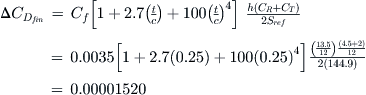
EXAMPLE 15-9
Determine the additive drag coefficient for a COM antenna for the SR22 airplane, if its root chord is 4.5 inches, tip is 2 inches, and height is 13.5 inches. Assume a skin friction coefficient of 0.0035 and an average thickness-to-chord ratio of 0.25.
15.5.5 Drag of Streamlined Struts and Landing Gear Pant Fairings
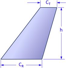
The cross-sections in Figure 15-46 are typical of those used for wing struts or to reduce the drag of leaf-spring landing gear legs. Such shapes typically operate in a low Re region, where the Re is based on their chord, denoted by c. The drag of such sections is typically related to their thickness-to-chord ratios.
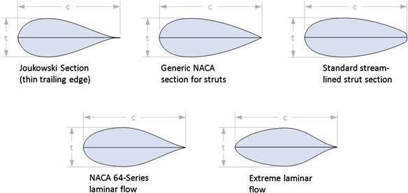
FIGURE 15-46 Selected standard cross sections for wing and landing gear struts. (reproduced from Ref. [3])
The additional drag coefficient for the strut, ΔCDS, is given by Hoerner [3, p. 6-5] and is based on empirical results:
![]() (15-85)
(15-85)
where
The miscellaneous drag coefficient for a strut of length L and chord c in terms of Sref would thus be estimated from:
![]() (15-86)
(15-86)
Note that this would be the contribution of the strut to the total miscellaneous drag. Also note that since all the cross-sections have the same form factor, the difference comes in the evaluation of the skin friction coefficient, Cf.
EXAMPLE 15-10
Determine the additive drag of a (Cessna-like) wing strut whose length is 5 ft, chord is 4 inches, and t/c is 0.2 at S-L at airspeed of 110 KTAS. The reference area is 160 ft2. Assume no interference and Cf = 0.008.
Solution
Using Equation (15-86) we get:
![]()
This amounts to about 6.2 drag counts. Therefore, the resulting drag amounts to:
![]()
This means that each strut (assuming there are two) adds 3.34 lbf of drag to the total drag.
EXAMPLE 15-11
Determine the additive drag coefficient of a step onto the wing to help occupants enter the cabin of an SR22 aircraft. There are two such entry steps, whose cross-section is the standard streamlined strut section that are approximately 12 inches long, 3-inch chord and 1-inch thickness. Assume no interference, ignore the break in the step where it changes from a step to a strut and Cf = 0.008.
Solution
The t/c is about 1/3 = 0.333. Therefore, using Equation (15-86) we get for each step:
![]()
This amounts to about 2.28 drag counts.
Thick Fairings
A fairing is a streamlined structure whose purpose is to reduce the drag that would be caused by the underlying geometry. Hoerner [3, p. 6-9] presents the following expression to determine the (two-dimensional) drag of a fairing whose chord is c, height is t, and length is L:
![]() (15-87)
(15-87)
The term inside the parenthesis is the form factor. It accounts for pressure and friction (see Figure 15-47). This means of course that for a strut of length L and chord c in terms of Sref would thus be estimated from:
![]() (15-88)
(15-88)
This allows the optimum thickness-to-chord ratio to be determined by determining the derivative, setting it equal to zero, and solve for the optimum t/c, as shown below:
![]()
Therefore, the optimum thickness-to-chord ratio is 0.273. This corresponds to a fineness ratio of ≈ 3.7.
15.5.6 Drag of Landing Gear
Drag of Tires Only
Figure 15-48 shows several types of aircraft tires, identified as A, B, C, and D. The drag generated by these styles is the topic of NACA R-485 [32]. It is convenient to express the drag coefficient of tires in terms of their frontal area, which is defined as their diameter, d, multiplied by their width, w. This has been done in Figure 15-48 and Table 15-9. The additive drag coefficient of the tire can be estimated from:
![]() (15-89)
(15-89)
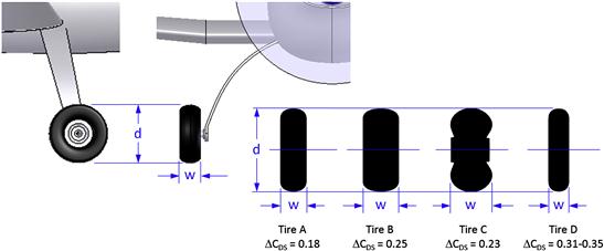
FIGURE 15-48 Most common types of modern tires for aircraft landing gear. (based on Ref. [32])
Drag of Tires with Wheel Fairings
The purpose of wheel fairings is to improve the aerodynamic geometry of the tire and thus reduce its drag. Figure 15-49 shows several fairing styles and Table 15-10 lists the applicable drag coefficients based on (1) the frontal area of the fairing and (2) the frontal area of the tire. It is left to the reader to select which one to use. While the data is based on a Type III tires, for preliminary design purposes it may be assumed the drag coefficients are independent of the type of tire. The additive drag coefficient of the tire with the fairing can be estimated from:
![]() (15-90)
(15-90)
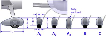
FIGURE 15-49 Selected types of landing gear wheel fairings (based on Ref. [32]). The drag of the landing gear wheel fairing styles denoted by “A” through “C” is presented in Table 15-10.
TABLE 15-10
Drag of Tires with Fairings (H = Fairing Height, W = Fairing Width, d = Tire Diameter, w = Tire Width)

Note that this coefficient is for a single tire with a fairing. This is emphasized because some texts present the drag coefficient for two wheels (e.g. assuming both main landing gear). However, some aircraft feature fairings on the main wheel only, while others have all three wheels (main and nose landing gear) with fairings.
Drag of Fixed Landing Gear Struts with Tires
Drag coefficients for a number of typical fixed main landing gear with tires are presented in Table 15-10. All the drag coefficients are based on the dimensions of a single tire per side but apply to the entire installation (both wheels and support structure). The coefficients include interference drag, but exclude the nose landing gear, however. The additive drag coefficient of the fixed landing gear with the fairing can be estimated from:
![]() (15-91)
(15-91)
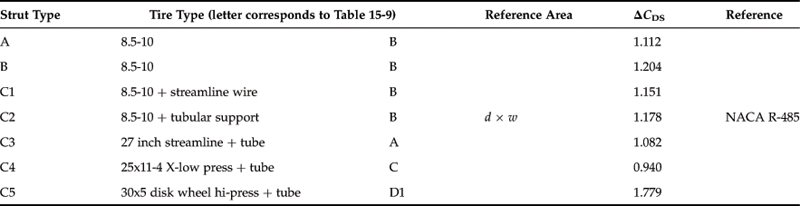
Refer to Figure 15-50 for the shape of the landing gear configuration. Each configuration is identified with a letter ranging from A to H. Reference [32] presents results for the said configurations, of which some feature more than one type of tire and even fairings. These differences are presented in Table 15-11 using numbers following the letter. Thus, configurations A and B both feature a Type III tire, whereas configuration C is presented with five different tires, one configuration of which is supported by a streamlined tension wire and the other by a tubular tension support. The remainder of the configurations utilize that same tubular support.
EXAMPLE 15-12
Determine the additive drag coefficient for the fixed landing gear of the SR22 airplane. Its wing area is 144.9 ft2 and assume the main landing gear tire dimensions are 15 inch diameter and 6 inch width and the nose gear tire is 14 by 5 inches.
Solution
Approximate the main landing gear using Configuration I2 since the landing gear fairing (Style C) is similar in some ways to that of the SR22. The additive drag coefficient for I2 is ΔCDS = 0.484. Similarly, assume the nose landing gear can be represented using Configuration M1, for which ΔCDS = 0.484 as well. In this case note that the drag refers to the entire installation, which consists of two wheels. Since the nose gear is a single wheel, we reduce this number by a factor of two, i.e. ΔCDS = 0.242 for the nose gear. Thus we estimate the drag contribution of the main and nose landing gear to be represented by (note that a factor of 144 is used to convert in2 to ft2:
![]()
![]()
This amounts to about 20.9 drag counts due to the main gear and 8.1 counts due to the nose landing gear.


FIGURE 15-50 Drag of selected types of fixed landing gear installations. All struts are streamlined. All drag coefficients are based on the tire geometry and pertain to the entire installation (two main gear) (based on Refs [23] and [32]). The drag of the fixed landing gear installation styles denoted by “A” through “Q” is presented in Table 15-11.

Drag of Retractable Landing Gear
Austyn-Mair and Birdsall [33] give the following empirical expressions for the additive drag of landing gear in the absence and presence of flaps. In other words, one expression applies to the landing gear down and flaps retracted, the other to the both the landing gear and flaps extended. The equations are based on historical data and are presented in terms of weight, W (in lbf) in the UK system, or mass, m (in kg) in the SI system. They are representative of commercial jetliners and business jet, and should not be used with lighter GA aircraft. The drag of landing gear with the flaps stowed is given as follows in the SI and UK systems, respectively:
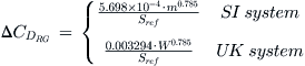 (15-92)
If the flaps are fully deflected the expression becomes:
 (15-93)
EXAMPLE 15-13
Determine the additive drag coefficient of the retractable landing gear for an airplane that weighs 22000 lbf and whose wing area is 300 ft2, with and without flaps.
Jenkinson et al. [34] give the following expression for the drag of the landing gear of commercial jetliners. Formulation for two classes of jetliners is given; for medium to large jetliners like the Boeing 747, 757, 767, DC-10, L-1011, etc. and for smaller jetliners, such as the F-100, DC-9, and B-737. The expressions are presented in terms of the flat plate area, ΔD/q. However, these have been modified to adhere to the presentation in this book.
where WNLG and WMLG is the weight of the nose and main landing gear, respectively (in lbf) and mNLG and mMLG is the mass of the nose and main landing gear, respectively (in kg).
Roskam [23] presents a simple method for determining the additive drag of retractable landing gear. It uses the ratio of the actual frontal area of the landing gear to the area of a rectangle enclosing the gear to calculate the additive drag coefficient (see Figure 15-51). The method assumes an open wheel well, but suggests a 7% reduction to correct for closed wells. The resulting formulation is presented below, for configurations with both open and closed wheel wells:
![]() (15-96)
(15-96)
![]() (15-97)
(15-97)
Note that even though the drag coefficient is based on the aforementioned ratio of the actual frontal to enclosed area of one wheel, the value of ![]() applies to both legs of the main landing gear (the nose landing gear is not included). Also note a common error is to forget to convert d and w (which often are in inches) to ft, to ensure unit consistency with Sref in ft2.
applies to both legs of the main landing gear (the nose landing gear is not included). Also note a common error is to forget to convert d and w (which often are in inches) to ft, to ensure unit consistency with Sref in ft2.

FIGURE 15-51 Estimating the drag contribution of a retractable landing gear. (based on Ref. [23])
Drag of Nose Landing Gear
Drag of nose landing gear is presented in the graph in Figure 15-52. The method requires the distance of the gear from the nose, a, total length of the extended landing gear, e, and tire diameter, d, to be known. The ratio a/d is first determined and used to select the appropriate curve. Then the wheel height ratio, e/d, is calculated and used with the selected curve to read the drag coefficient on the vertical axis. Then, this can be converted into the additive drag coefficient, which is based on the reference wing area as follows:
![]() (15-98)
(15-98)
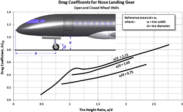
FIGURE 15-52 Estimating the drag contribution of a nose landing gear. (based on Ref. [23])
15.5.7 Drag of Floats
Floats are a popular option for many types of GA aircraft. Their primary drawback is a healthy dose of additive drag, inherent destabilizing moment, and weight. This section presents a method to estimate the drag. Reference [35] investigated the drag of four full-scale floats used as a single float for large single-engine military aircraft, such as the Vought OS2U Kingfisher. The floats varied in length, ranging from about 24.8 to 26.6 ft, with maximum cross-sectional area ranging from 6.63 to 9.25 ft2. While this is larger than what is typically used for most single engine GA aircraft, the results are ideal to use for estimating the drag of smaller floats. Among conclusions cited by the reference is that the step adds about 10% of the drag, adding a tail fairing reduced it by some 8%, and there was negligible benefit gained by using counter-sunk rivets versus normal universal-head rivets aft of the step.
The following expressions refer to the configurations A, B, and C, shown in Figure 15-53. The term Amax is the maximum cross-sectional area of the float and α is the AOA with respect to the horizontal upper surface. No provision was made to reduce the drag specifically, e.g. by removing hardware. The drag measurements included support fairings, except wire bracings were not present. The Reynolds number is 25 million, based on the length of the float. The drag was measure using an α-sweep from −6° to +6° at an airspeed of 87 KTAS. The drag applies to a single float only, so if using two floats the additive drag coefficient must be doubled:
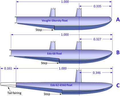
FIGURE 15-53 Float geometries (based on Ref. [35]). The drag of the float styles denoted by “A”, “B”, and “C” is presented in Equations (15-99), (15-100), and (15-101), respectively.
Reference [36] investigated special NACA-designed floats, referred to as the NACA 57 series. It was found that the dead rise angle (the angle between the horizontal and the “v” of the float) had a small effect on the total drag: the greater the dead rise angle the higher the drag. The drag coefficients increase with the AOA similar to that reflected by Equation (15-99); however, the minimum drag (ΔCDS) is less or about 0.13 to 0.155.
![]() (15-101)
(15-101)
15.5.8 Drag of Deployed Flaps
Deflecting flaps will introduce two modifications to the drag model: (1) the minimum drag will increase and (2) the lift induced drag will increase. This section introduced methods to account for this change.
Increase of CDmin Due to Flaps
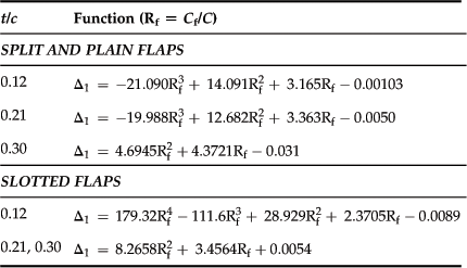
Young [37] presents an empirical method to estimate the drag of a number of types of flaps. The estimation depends on the flap type, flap chord (Cf), deflection angle (δf), and its span (bf). The following expression is used for this estimation and it requires the two functions Δ1 and Δ2 to be determined. The former accounts for the contribution of the flap chord to the flap drag and the latter for the contribution of the flap deflection. These are detailed in the two graphs of Figure 15-54, and are discussed further below.
![]() (15-102)
(15-102)

FIGURE 15-54 Estimation of the drag contribution of the flaps calls for the Δ1 and Δ2 functions to be determined. (based on Ref. [37])
The Function Δ1
As stated earlier, the Δ1 function represents the contribution of the flap chord to the flap drag. This contribution is shown in the left image of Figure 15-54, for plain, split, and slotted flaps, for airfoils of three thickness-to-chord ratios; 0.12, 0.21, and 0.30. These graphs have been digitized from the original document and can be reconstructed using the polynomial curve-fits shown in Table 15-12. Note that the parameter Rf is the flap chord ratio, i.e. Rf = flap chord/wing chord = Cf/C. This ratio typically ranges from 0.20 to 0.35.
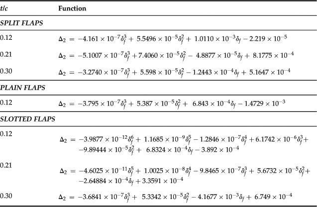
The Function Δ2
The Δ2 function represents the contribution of the flap deflection angle to the flap drag, shown in the right image of Figure 15-54, for plain, split, and slotted flaps, for airfoils of three thickness-to-chord ratios; 0.12, 0.21, and 0.30. These are given by the polynomial curve-fits shown in Table 15-13.
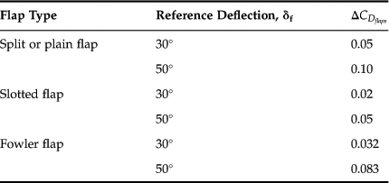
Corke [38] presents additive drag for several types of flaps at the 30° and 50° deflection. These are reproduced in Table 15-14. It is a limitation that these apply to the specific flap span and chord of 60% and 25%, respectively. However, these can come in handy for initial estimation of flap drag.
TABLE 15-14
Additive Flap Drag Coefficients (Based on Ref. [38]): Assumes 60% Flap Span and 25% Chord
15.5.9 Drag Correction for Cockpit Windows
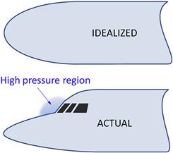
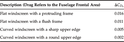
The fuselage form factor estimation methods presented earlier assume a fuselage with a smooth round forward geometry that provides a smooth contour for air to flow across. Such smoothness is normally not achieved in airplanes; they often feature a sharp discontinuity around the cockpit windows. Cockpit windows are often flat, in particular in pressurized aircraft, which have heated windscreens for improved bird-strike resistance and to minimize optical distortion.
Drag of Conventional Cockpit Windows
A consequence of this discontinuity is a high-pressure region, caused by the reduction in airspeed over the geometry. This increases the drag of the airplane, which is corrected using an additive drag contribution. Reference [23] presents such a method, assuming the general geometry shown in Figure 15-55. The drag coefficients refer to the maximum frontal area of the fuselage (Amax), which can be estimated using a method such as that shown in Figure 15-35. The source drag coefficients are given in Table 15-15.
![]() (15-103)
(15-103)
EXAMPLE 15-14
Estimate the additive drag of the SR22 due to the cockpit window, assuming a curved windscreen with a round upper edge. The fuselage cross-sectional area is approximately 14 ft2.
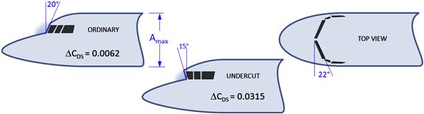
Drag of Blunt Ordinary and Blunt Undercut Cockpit Windows
A cockpit window installation can be classified as blunt if the windscreen faces the oncoming airflow at angles ranging from normal to around 22° in the horizontal plane and ±20° from the vertical, as shown in the top and side views of Figure 15-56, respectively. The vertical angle is used to define the ordinary and undercut configurations. Generally, the blunt installation leads to higher drag than conventional curved geometry. In particular, note that the undercut installation, a popular approach in the 1930s to reduce the reflection of instrument lights at night (e.g. on the Boeing 247 [39] and the Vultee V-1), is a very draggy configuration and should be avoided by any means. The source drag coefficients shown in the figure are used with Equation (15-103).
15.5.10 Drag of Canopies
Many single- to four-seat aircraft are designed with canopies rather than roofed cabins to improve the field-of-view. This section presents a simple method to estimate the drag caused by such geometric protrusions. It is based on experimental data presented in Ref. [40], in which a number of dissimilar canopies were investigated at Mach numbers ranging from 0.19 to 0.71 and AOAs up to 6°. The geometric representations of the canopies are shown in Figure 15-57. The reference found that the contribution of a well-designed canopy to the total drag of the airplane was approximately 2% of the total drag, whereas a poorly designed one could easily exceed that 10-fold – and be 20% of the total drag. This shows that awareness of canopy drag is of great importance in the aircraft design. The drag is presented in terms of the maximum cross-sectional area of the window, Amax, using the following expression:
![]() (15-104)
(15-104)

FIGURE 15-57 Canopy styles evaluated by Ref. [40]. The drag of the canopy styles denoted by “A” through “I” is presented in the graph of Figure (15-58).
The values of the ΔCDs for the various canopy geometries are shown in Figure 15-58, plotted for the cited range of Mach numbers. This data is only provided for a low AOA, although information for higher AOAs (up to 6°) is provided in the reference document. The lower AOAs are likely to be of greater interest to the designer of efficient aircraft featuring canopies. However, if the design mission involves prolonged cruise at or near LDmax or high-speed maneuvers (where compressibility effects prevail), the higher AOAs become important. The reference also presents the distribution of pressure coefficients, allowing for the estimation of critical Mach number (see Section 8.3.7, The critical Mach number, Mcrit).
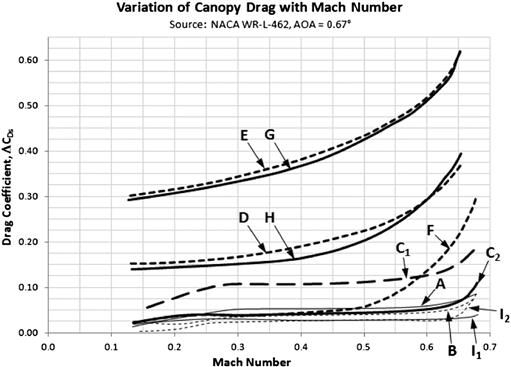
FIGURE 15-58 Drag coefficients for the canopy styles of Figure 15-57. (reproduced from Ref. [40])
15.5.11 Drag of Blisters
Hoerner [3, p. 8-5] collected information on drag for various shapes of blisters from a number of sources. Blisters are fairings that cover components that extend beyond the original outside mold line. Blisters are ideal when estimating the drag of GPS antennas. The drag of blisters can be calculated from:
![]() (15-105)
(15-105)
where Amax = cross-sectional area of shape as shown in Figure 15-59.
EXAMPLE 15-15
Estimate the additive drag of a GPS blister antenna for the SR22, assuming a length × width × height of 4.7 × 3.0 × 0.78 inches. Assume the base (e) is 30% of the width (b) and that its side view resembles that of the top blister in Figure 15-59. Furthermore, assume a maximum cross-sectional area of 14.1 in2.
Solution
The height ratio is about 0.78/4.7 = 0.17, so it is a tad outside the limits cited in Figure 15-59. However, since it is fairly close, we will assume the drag can indeed be estimated using Equation (15-105).
![]()
This amounts to approximately 0.33 drag counts. Note this antenna is about two times “draggier” than the wing shaped antenna of Example 15-9.
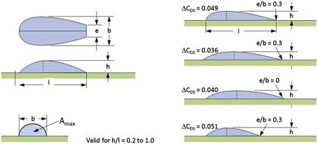
FIGURE 15-59 Drag contribution of typical blisters (bumps). (based on Ref. [3])
15.5.12 Drag Due to Compressibility Effects
Drag due to drag divergence was introduced in the Section 15.4.2, The effect of Mach number. The following method can be used to account for this drag increase at high Mach numbers, provided the three following parameters are known: (1) the critical Mach number, Mcrit, (2) the maximum drag due to Mach drag divergence, ΔCDmax D, and (3) the Mach number at which it occurs, Mmax D (see Figure 15-60). If these are known, the additional drag for Mach numbers ranging from 0 to Mmax D can be estimated using the following expression:
![]() (15-106)
(15-106)
where M is the Mach number and the constants A and B are determined using the following expressions:
![]() (15-107)
(15-107)
![]() (15-108)
(15-108)

The beauty of this method is that the compressible drag contribution can be used as an additive drag component for any Mach numbers as long as it is less than Mmax D. This is convenient for programming or spreadsheet use, as it helps avoiding having to feature IF statements to control when this component is added to the incompressible drag. (Note that ΔCDM is added to the sum of miscellaneous drag contributions like any other in this section.)
Derivation of Equations (15-106) through (15-107)
![]()
Since the hyperbolic tangent has asymptotes at y = −1 and y = 1, it is necessary to divide ![]() by 2 (because the asymptotes are separated by a value of 2). The value “1” is used to shift tanh vertically, so the lower asymptote will be at y = 0, rather than y = −1. The function can be used as a spline to approximate the drag divergence by determining the constants A and B such the function goes through some specific points on the drag versus Mach curve (see Figure 15-28). These points are: (1) Mcrit, where the drag begins to rise and (2) Mmax, where it reaches its maximum value,
by 2 (because the asymptotes are separated by a value of 2). The value “1” is used to shift tanh vertically, so the lower asymptote will be at y = 0, rather than y = −1. The function can be used as a spline to approximate the drag divergence by determining the constants A and B such the function goes through some specific points on the drag versus Mach curve (see Figure 15-28). These points are: (1) Mcrit, where the drag begins to rise and (2) Mmax, where it reaches its maximum value, ![]() . To work around the lower asymptote, we assume a very small increase in
. To work around the lower asymptote, we assume a very small increase in ![]() at Mcrit; Here we will assume 1 drag count or 0.0001. To work around the upper asymptote, where
at Mcrit; Here we will assume 1 drag count or 0.0001. To work around the upper asymptote, where ![]() reaches its maximum value (
reaches its maximum value (![]() ) we assume its value is
) we assume its value is ![]() . Therefore, we can write:
. Therefore, we can write:
We readily see that we can solve for the argument of the hyperbolic tangent as follows:
![]()
This allows us to write:
Solving for A and B, thus, yields Equations (15-107) and (15-108).
QED
15.5.13 Drag of Windmilling and Stopped Propellers
Drag Due to Windmilling Propellers
A windmilling propeller is usually associated with an engine failure in flight. Compounding the loss of thrust is a large amount of drag added to the airplane. This can create a serious problem for its continued operation. For single-engine aircraft, the added drag is a serious detriment to its glide capability. For multi-engine aircraft it severely reduces range and contributes to the asymmetric moment that must be balanced by rudder and aileron deflection.
The rotating propeller acts as a wind turbine that drives the engine and must develop enough torque to overcome the internal friction of the engine. A thorough analysis of the phenomenon is beyond the scope of this book, but some experimental data is provided in Ref. [41]. The following methods are provided for initial estimation only.
Hoerner [3] suggests a method in which the power required to turn the engine is 10% of its rated power and the propeller efficiency expected through the windmilling is of the order of 50%. In other words, 50% of the drag power is converted into the rotational power. This allows us to write:
![]()
Assuming the windmilling drag to depend on dynamic pressure and propeller disk, we can write:
![]()
Inserting this into the previous expression, solving for the drag coefficient and referencing it to the reference area yields:
![]() (15-109)
(15-109)
where V is the glide speed and ρ the density at condition. Comparison to existing aircraft reveals that Equation (15-109) over-predicts the additive drag by a factor of 2 to 4. For this reason, for small engines with low internal friction multiply the value by 0.25 and for larger engines with a high internal friction multiply by 0.33. The author’s unpublished study of single-engine aircraft reveals that windmilling propellers increased drag by approximately:
![]() (15-110)
(15-110)
with several excursions nearing and even exceeding 300 drag counts! The above value will easily reduce the LDmax of a sleek airplane by a whopping one-third.
Drag Due to Stopped Propellers
If the propeller of a malfunctioning engine does not windmill, but stops, the drag will indeed be less. It is possible to estimate the drag of such propellers based on the planform area of the blades, assuming they generate drag similar to a flat plate at a specific blade angle. In this context, the blade angle is defined as the angle between the chord of the blade airfoil at 0.7 radius to the rotation plane. The angle is close to the pitch angle of the airfoil (e.g. see Figure 14-9). Thus, when the angle is zero, the blade drag is high and when low, the drag is much lower. Hoerner [3], citing experiments from Ref. [41], provides the following expression to estimate the drag coefficient of such a blade:
![]()
where β is the blade angle at the 0.7 radius and which may or may not be equal to the pitch angle referenced in Chapter 14, The anatomy of the propeller. This shows the blade drag coefficient varies between 0.1 and 1.1. This allows the drag of the stopped propeller, denoted by Dsp, to be written as follows:
![]()
where Nblades is the number of blades and Sblade is the planform area of the blade. Solving for the drag coefficient that uses the reference area (Sref) and is denoted by ΔCDsp, yields the following expression:
![]() (15-111)
(15-111)
15.5.14 Drag of Antennas
There are typically three kinds of antenna geometries planted on aircraft: (1) blister type, (2) wire type, and (3) wing type. Their drag can be estimated using the methods already presented in here. Typical placement and shapes of such antennas is shown in Figure 15-61. Their number can easily turn your nice, smooth airplane into something resembling a porcupine! If possible, try to mount as many antennas internally as practical, although often this is impossible due to reduced effectiveness of the antenna. Also, ask the manufacturer for an additive drag coefficient associated with their antenna: some have this readily available – it may save you analysis work. Others do not and for those you will have to estimate the drag based on the geometry using the approximations below.

15.5.15 Drag of Various Geometry
Figure 15-62 shows the three-dimensional drag coefficient for a sphere and a circular cylinder, based on Schlichting [4]. The drag coefficient is defined using Equation (15-78), where SS is the cross-sectional area (πD2/4 for the sphere and D·L, where L is the length of the cylinder). Schematics showing the nature of the separation have been superimposed to demonstrate how the drag coefficient depends on the nature of the flow separation that occurs. The dashed line indicates a specific region where the said flow nature takes place. Of importance is the sharp dip near a Re of 300,000 (sphere) and 500,000 (cylinder), first discovered by Alexander Gustave Eiffel (1832–1923).5 This dip is indicative of the formation of a turbulent boundary layer that better follows the geometric shape of the solid, reducing the size of the wake and, thus, the pressure drag generated by the object. The figure also shows the relatively constant drag coefficient of geometry over the range 103 < Re < 105, but this is indicative of the formation of a laminar boundary layer (as long as the surface is smooth).
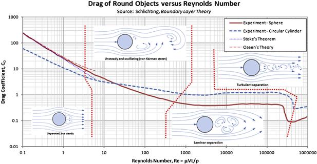
FIGURE 15-62 The drag coefficient of a sphere and a circular cylinder as a function of Re. Inserts are schematics showing the nature of the separation, whose consequence is the CD shown in the graph.
The range of Re starting at 103 and above is of great interest to the aircraft designer because this covers most airplanes, even small radio-controlled aircraft. This region is usually broken into four separate sub-regions called subcritical, critical, supercritical, and transcritical (see Figure 15-63).
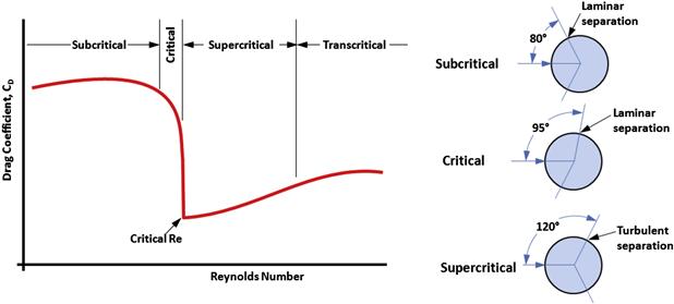
In the subcritical region, laminar boundary layer is formed that separates once it flows to latitude of approximately 80° (see the schematic to the right in Figure 15-63). As stated above, the CD in this range (103 < Re < 105) is practically constant (i.e. independent of the Re). In the critical region, the CD drops sharply over a relatively narrow range of Re, reaching a minimum value called the critical Reynolds number. This drop is caused by a sudden movement of the laminar boundary layer separation point to latitude of almost 95°. At the critical Re, a separation bubble is formed at this location that forces the laminar boundary layer to separate into a turbulent one. This, in turn, can more easily follow the shape of the geometry, moving the separation point farther downstream to approximately 120°. This dramatically reshapes the separation region, reducing its diameter and consequently the pressure drag, which explains the reduction in the drag coefficient. In the supercritical region, laminar-to-turbulent transition occurs in the attached boundary layer, causing the separation to begin to crawl upstream, slowly increasing the drag coefficient again. In the transcritical region the transition point has moved upstream closer to the stagnation point, eventually causing the drag to become independent of the Re.
Figure 15-64 and Figure 15-66 show drag coefficients for selected geometry reproduced from Hoerner [3].

FIGURE 15-64 Two-dimensional drag coefficients of several cross-sections. Valid only for 104 < Re < 105.
Three-Dimensional Drag of Two-Dimensional Cross-Sections of Given Length
Research shows that the drag coefficients for the two-dimensional shapes shown in Figure 15-64 depends on their fineness ratio, here denoted by h/d (shown on the triangular shape in the center, lower row). However, their drag is determined using their frontal areas. Thus, the drag of the shapes is calculated from:
![]() (15-112)
(15-112)
where d = thickness of shape as shown in Figure 15-64 and l = length of shape in the out-of-plane direction.
The Cross-Flow Principle
Hoerner [3] presents a very practical method to calculate the drag of wires that are inclined with respect to the airflow (see Figure 15-65). This is referred to as the cross-flow principle. It can be used to estimate the drag and lift of a tube or cylinder of a given length, l, and particular cross-section, whose two-dimensional drag coefficient is known. The formulation below is used to calculate the coefficients in terms of the reference wing area so it (primarily the drag) can be added directly to the miscellaneous drag coefficient.

Note that the absolute sign in Equation (15-115) guarantees the drag is always greater than zero. Also note that the inclination angle of θ = 90° means the cylinder is perpendicular to airstream.
The cross-flow principle is very helpful in determining the drag of external aircraft components, such as HF radio wire antennas.
![]() (15-113)
(15-113)
![]() (15-114)
(15-114)
![]() (15-115)
(15-115)
where θ = the angle of inclination (see Figure 15-65).
Drag of Three-Dimensional Objects
Figure 15-66 shows a number of three-dimensional objects and the corresponding drag coefficients. The drag of these objects is also based on the cross-sectional area normal to the flow direction. Thus, the cross-sectional area normal to the flow direction for the sphere is given by π·d2/4, where d is its diameter. In general, if SN denotes this area (i.e. SN = π·d2/4), the three-dimensional drag coefficient is calculated from:
![]() (15-116)
(15-116)

15.5.16 Drag of Parachutes
While the drag of parachutes may appear simple, in reality it is surprisingly complicated. Accurate estimation of parachute drag and the time history of the drag generated during deployment is a serious scientific discipline, applicable to a range of applications, including the deployment of re-entry parachutes or ejection seats.
Hoerner [3] provides a practical insight into the drag of parachutes. In general, the drag coefficient of inflated parachutes is based on simple geometric features, such as the height, diameter, and the projected frontal area of the inflated canopy. For initial sizing, the drag coefficient, CDparachute, can be estimated based on the aspect ratio (AR) of the parachute, defined as its inflated height, h, by the inflated diameter, d. This is shown in the graph of Figure 15-67, which shows the inflated drag coefficient as a function of h/d. An empirical expression based on the graph is given below. It is valid only for h/d < 1.1 and 105 < Re < 106, where Re is based on the inflated diameter. The maximum drag coefficient is obtained for an AR of 0.5, which represents a hemi-spherical geometry. Further increase of the AR will make the parachute partially “fill in” the flow separation region, which will reduce the drag coefficient until it reaches a theoretical minimum of 1.0.
![]() (15-117)
(15-117)

FIGURE 15-67 Drag coefficients of rigid objects shaped like parachutes. Valid only for 105 < Re < 106 and h/d < 1.1. (reproduced from Ref. [3])
The coefficient is then used to evaluate the total drag force of the parachute using the following expression, where S is the projected area of the chute and S = π·d2/4:
![]() (15-118)
(15-118)
EXAMPLE 15-16
The POH for the SR22 states that the “the airplane will descend at less than 1700 feet per minute with a lateral speed equal to the velocity of the surface wind.” The company website states the diameter of the canopy is 55 ft. This means that, at the gross weight of 3400 lbf, the airplane will not exceed 1700 fpm (or 28.3 ft/s). Using this information, determine the drag coefficient of the parachute.
Solution
Solve for CDparachute using Equation (15-118):
![]()
Note that the Reynolds number is close to 107.
15.5.17 Drag of Various External Sources
This section presents the drag of various external sources that are important when present on the design.
Drag of Sanded Walkway on Wing
As shown in Table 15-8, Ref. [30] indicates adding a sanded walkway (both sides of the fuselage) adds 0.0007 drag counts to the total drag. For this reason assume the following drag increase per side:
![]() (15-119)
(15-119)
Drag of Gun Ports in the Nose of an Airplane
NACA WR-L-502 [42] presents the results from drag analysis of the introduction of openings for eight machine gun barrels in a P-38 Lightning style fuselage. It found the drag increase amounted to 5 drag counts or 0.0005 total, based on the wing reference area. Based on this result it is possible to estimate drag increase per opening as follows:
![]() (15-120)
(15-120)
Drag of Streamlined External Fuel Tanks
External fuel tanks are a typical supply of additional fuel for military aircraft. However, they are also a plausible solution to a long-range operation of some GA aircraft. A similar shape is often used to house weather radars for GA aircraft. It is for this reason their drag is presented here.
The drag of streamlined tanks is highly dependent on the interference of between the tank and the wing. Careless installation can easily increase drag by a factor of four, as shown in Figure 15-68. The installation should always be improved using streamlined fairings. The drag coefficients shown in the figure are based on the frontal area of the tank, Stank, and are related to the reference area as follows:
![]() (15-122)
(15-122)
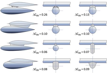
FIGURE 15-68 Drag of external fuel tanks (based on Ref. [3]). Note that the bottom configuration also resembles geometry often used to house wing mounted weather radars for small GA aircraft.
Drag Due to Wing Washout
Horner presents the following expression to account for increase in the lift-induced drag of a wing as a consequence of wing washout. It has been shown in Chapter 8, The anatomy of the wing, how the lift-distribution is altered as wing twist is introduced. This can lead to an appreciable lift-induced drag, even when the wing is at an AOA for which no lift is generated.
![]() (15-122)
(15-122)
where
ϕtip = angle of the tip with respect to the root of the wing, in degrees
ϕMGC = angle of the MGC with respect to the root of the wing, in degrees
So the angular difference is between the wingtip and the airfoil at the MGC.
Drag Due to Ice Accretion
Drag due to ice accretion on the aircraft as a whole poses a very serious challenge to safe flight. All aircraft can be classified as those that have been certified for flight into known ice (FIKI) and those that have not. Of course, all aircraft, regardless of classification, can accrete ice during operation. The problem of ice formation was studied at least as early as 1938 by Gulick [43], who found that the section drag coefficient of the airfoil studied almost doubled and the maximum lift coefficient reduced from 1.32 to 0.80, without changing the angle of stall. Further research took place in the early 1950s (e.g. see a paper by Gray and Glahn [44]). Since then, tremendous research effort has been dedicated to the subject. In fact, the sheer volume of papers that has been published cannot be adequately presented here. The interested reader is directed toward work done by NASA and AIAA.
15.5.18 Corrections of the Lift-Induced Drag
Wingtip Correction
In addition to the effect of AR and λ, the lift-induced drag is also affected by the wingtip geometry. As soon as the low- and high-pressure regions form on the wing, respectively, a vortex begins to form at each wingtip (see Figure 15-23). High pressure on the lower surface of the wing moves in a spanwise direction outboard and “rolls” over the wingtip toward the low-pressure region on the upper wing. Generally, it is assumed that the distance between the core of the two vortices equals that of the wingspan. However, in reality the wingtip affects how the roll-up of the vortices takes place (see Figure 15-69). Thus, the three-dimensional flow field is modified by the wingtip geometry and this shifts the wingtip vortices inboard or outboard with respect to the wingtip. If the separation of the wingtip vortices is increased in this manner, it is akin to increasing the AR of the wing. Similarly, if the separation of the vortices is decreased, it is as if the AR has been reduced.
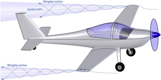
FIGURE 15-69 Pressure difference between the upper and lower surfaces forms the wingtip vortex, as the high-pressure field on the lower surface “rolls” over the wingtip toward the low-pressure field on the upper surface.
Hoerner [3, p. 7-5] presents a number of wingtips and their empirical effects on the AR of the wing, reproduced in Figure 15-70. The terms ΔAR are values that should be added to the geometric AR. The resulting value is then used when calculating lift-induced drag, CDi. For instance, consider a wing whose AR is 7. The selection of a round frontal view and round top view shows a ΔAR = −0.20. Therefore, the AR to use with Equations (15-45) and (15-47) would be 6.8 and not 7. Generally, the figure shows that rounded tips reduce the effectiveness of the wing – it is simply better to feature a square rectangular tip. It is cheaper too. Other wingtips are presented in Section 10.5, Wingtip design.
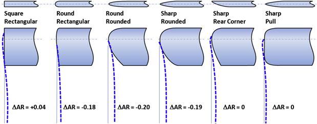
FIGURE 15-70 Effect of several types of wingtips on the separation of the cores of the wingtip vortices. Tested at Re = 1 × 10⁶ and AR = 3. (reproduced from Ref. [3])
The effect of how the wingtip shape influences the lift induced drag is based on how air flows around the wingtip. Three examples are shown in Figure 15-71. The top wingtip shape is round. It allows air to flow to the upper surfaces so the vortex core resides inside and on top of the wingtip. This results in a wingtip vortex that is closer to the plane of symmetry than the physical wingtip, effectively reducing the wingspan. The center wingtip is square. It forces the spanwise flow component of the lower surface to make the turn around a very sharp corner. This forces the vortex core to reside farther away from the plane of symmetry than the actual wingspan – it increases the effective wingspan, albeit by a fraction. The bottom wingtip is representative of the so-called Hoerner wingtip. It promotes spanwise flow outboard and upward that is forced to make a turn around a sharp corner.
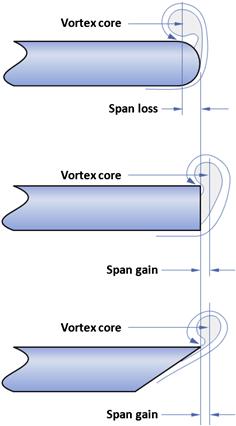
This forces the vortex core to reside even farther outboard than the square wingtip in the middle. This idea is extended to the so-called upturned or downturned booster wingtip that helps place the vortex such that a small effective wingspan increase is achieved, although this is not always realized in practice.
Correction of Lift-Induced Drag in Ground Effect
As shown in Section 9.5.8, Ground effect, the lift-induced drag is reduced when the aircraft is operated close to the ground. This fact should be taken into account during T-O and landing analysis. The effect is favorable during the T-O ground run as the total drag of the airplane is reduced. It is unfavorable during the landing ground roll, for the same reason. Use any of the methods in the section to correct the lift-induced drag based on the height if the MGC above the ground.
EXAMPLE 15-17
(a) Evaluate the complete minimum drag coefficient of the SR22 assuming the results from the component drag build-up method of Example 15-6, and the various additive drag contributions evaluated in this section. How does it compare to the CDmin = 0.02541 calculated from published performance information?
(b) Perform this evaluation at other altitudes as well (only change will be in the skin friction). How will this affect the CDmin?
Solution
See Table 15-16 for the result and the discussion that follows:
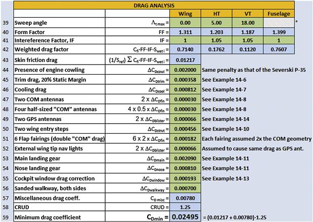
The table shows the estimated drag is in reasonable agreement with the one reverse-engineered from published performance data, as it is 100 × 0.02495/0.02541 = 98.2%. There are many areas that one can argue could be refined; for instance the airplane’s tie-down rings and control surface gaps are not included. These would add to the total. On the other hand, it is debatable whether a 20 drag counts penalty due to the presence of the engine cowling is justifiable (see row 44 in the table). This penalty is attributed to the fact the front part of the airplane features a cowling with an inlet and exit, which generates substantially higher drag than the smooth nose shape assumed by the fuselage skin friction estimation of Example 15-6. The 20 drag counts in row 44 were based on an airplane (the P-35) that has a radial engine. This should be expected to have higher drag than the horizontally opposed piston engine of the SR22. The important point is that while a careful prediction ought to put one in the neighborhood of the drag obtained by experiment, any contribution should be carefully reviewed and justified.
(b) Since the drag analysis was prepared in a spreadsheet, it is easy to change the altitude and get a new estimate. This has been done for altitudes ranging from S-L to 14,000 ft and this is shown in the left graph of Figure 15-72. The flight test value of CDmin = 0.02541 is shown as the vertical dashed line. Interestingly, this value was obtained using cruise data at 8000 ft (see Example 15-18). The right graph of Figure 15-72 shows the contribution of various sources of drag at two airspeeds. Note the large contribution of the lift-induced drag the lower airspeed.

15.6 Special Topics Involving Drag
Sometimes it is necessary to extract drag (reverse-engineer) from existing airplanes to validate the estimates of a new design of a similar geometry. This section presents several methods for this purpose. Of course there are several shortcomings to these methods and some extract less data than others. All the methods assume either the simplified or adjusted drag models of Section 15.2, The drag model. Drag characteristics featuring drag buckets require a large number of data and even wind tunnel testing and are not treated by the methods below. For this reason, applying the methods in this section to sailplanes is erroneous (even though one such is presented as an example later in this section).
The reader must use both caution and sound judgment when extracting numbers, as units, such as those for airspeed, are often ambiguous. Thus, the context of the units must be understood. Sometimes numbers come from advertising brochures which have been prepared by the marketing department. Such documents usually feature artistic presentation that is pleasing for the eyes, but sparse on details. They are often prepared by graphic artists who are not pilots themselves, let alone engineers. For instance, airspeed is commonly presented using knots. To such a person a knot is a knot. However, to an engineer (and pilots) a knot is not just a knot. There is a huge difference between an indicated knot (KIAS), a calibrated knot (KCAS), and a true knot (KTAS). The lack of detail in the preparation of advertising documents forces the engineer to apply sound judgment when using such numbers and the type of knot must be inferred from the type of airspeed.
If confronted by such a predicament the reader should be mindful that marketing departments thrive on extremes. They want to report the highest this or the lowest that, so they can separate their product from the competition. For instance, we want our airplane to have a low stalling speed and a high cruising speed. Knowing this, advertising brochures will report the stalling speed using KCAS because it is lower than the KTAS value (assuming the airplane is stalled at some altitude above ground). This is of course justifiable, because pilots want to know the indicated stall speed (KIAS) and by assuming low instrument and position error (approximately ±3 knots or so) one can get an idea of the airplane’s low-speed capabilities. Therefore, stalling speeds reported as kts (e.g. 42 kts) in such brochures should be assumed to reflect knots calibrated airspeed (i.e. 42 KCAS). On the other hand, marketing departments want the cruising speed to appear as large as possible and will therefore use KTAS because that number is much larger than the corresponding KCAS (or the KIAS) value, in particular if the airplane cruises at high altitudes. Again, this is justifiable because the pilot or the customer may want to know how long it will take to fly certain distances and the true airspeed is needed for that assessment. Therefore, a cruising speed reported as kts (e.g. 180 kts) in such a brochure should be assumed to reflect knots true airspeed (i.e. 180 KTAS).
15.6.1 Step-by-step: Extracting Drag from L/Dmax
The simplest method uses the L/Dmax and the airspeed at which it is achieved. This information is commonly available from aircraft Pilot’s Operating Handbooks (POH) and is almost always based on actual flight testing. The information this particular method extracts is the CDmin, and assumes the UK system of units. It is a limitation of the method that it uses the simplified drag model. However, since the CLminD will only shift the drag polar sideways (see Section 15.2.2, Quadratic drag modeling) there really is no error introduced in the extraction of the CDmin. Another issue is the extraction of drag for propeller powered aircraft. The L/Dmax reported in the POH will include drag from the windmilling propeller (since the purpose is to present the pilot with potentially life-saving information). This can easily double the minimum drag coefficient when compared to the other methods in this section and renders it much higher than required for accurate performance analyses. Therefore, care must be exercised when using these numbers.
Step 1: Gather Information from the Vehicle’s POH
Assuming the user has access to the aircraft’s POH, gather the following information: gross weight (W0) in lbf, best glide airspeed (VLDmax), wing area (S) in ft2, and wing aspect ratio (AR). If AR is not known, use wing span (b) in ft and compute it from b2/S.
Step 2: Convert VLDmax into Units of ft/s
Note 1: It is important that consistent units are used. Therefore, if V is read in KTAS is must be converted to ft/s. Similarly, if VV is given in fpm (ft/min) it must be converted to ft/s. Use the following conversion factors:
Note 2: Often the POH will report the best glide airspeed in units of KIAS or KCAS. This must be converted to KTAS for this method is to be applied at altitude (see Section 16.3.2, Airspeeds: instrument, calibrated, equivalent, true, and ground airspeeds, for methods).
Step 3: Calculate the Best Glide Lift Coefficient
Calculate the lift coefficient at the best glide speed from:
![]()
Step 4: Calculate Span Efficiency
Estimate the span efficiency, e, from any of the methods of Section 9.5.14, Estimation of Oswald’s span efficiency.
Step 5: Compute Minimum Drag
Compute the minimum drag from the following expression:
![]() (15-123)
(15-123)
Derivation of Equation (15-123)
The simplified drag model is given by:
![]()
Knowledge of the lift-to-drag ratio at a specific condition (here conveniently selected to be the LDmax, since aircraft manufacturers so graciously report this for us), and the lift coefficient associated with it can then be used to extract the minimum drag coefficient.
![]()
QED
15.6.2 Step-by-step: Extracting Drag from a Flight Polar Using the Quadratic Spline Method
This method can be used if the flight polar (or rate-of-sink versus airspeed or VV versus V plot) is available, as it often is for sailplanes, gliders, and motor gliders. Usually, this polar is not available for powered airplanes. It can be used to extract CDmin, CLminD, and e. This method will not retrieve a drag model that features a drag bucket, but a quadratic one. Also, it is important the reader reviews Appendix E.5.7, Quadratic curve-fitting, for further clarification of the method used here.
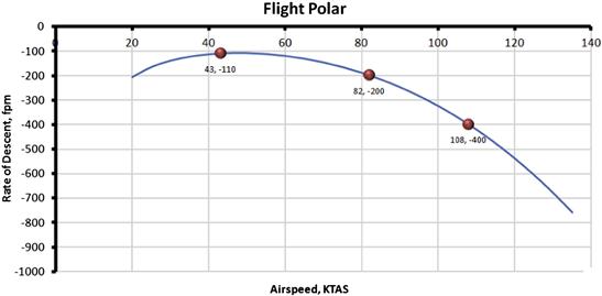
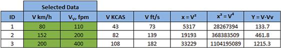
Consider the sample flight polar in Figure 15-73. Follow the following the stepwise procedure to extract CDmin, CLminD, and e.

Step 1: Select Representative Points from the Flight Polar
Select three arbitrary points on the flight polar and record the corresponding VV and V. For instance, select two points that enclose the minimum (near 50 KTAS in Figure 15-73) and one at a higher speed, for instance near 100 or 120 KTAS.
Step 2: Tabulate
Fill in the table below by entering the V and VV selected in Step 1 in columns 1 and 2 below. Calculate the values in columns 3 though 5.
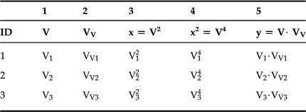
Note 1: It is important that consistent units be used. Therefore, if V is read in KTAS is must be converted to ft/s. Similarly, if VV is given in fpm (ft/min) it must be converted to ft/s. Use the conversion factors shown under the Note 1 of Step 2 of Section 15.6.1, Step-by-step: Extracting drag from L/Dmax:
Note 2: This formulation is based on the use of the absolute value of the rate-of-sink. If the VV is reported with a negative sign it must be converted to a positive number.
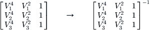
Step 3: Fill in the Conversion Matrix and Invert
Fill in the matrix below using the values in column 4 for the first row in the matrix and column 3 for the second row. This order is imperative. Then, invert the matrix. This can be done by some software, for instance, any spreadsheet software will offer means to invert matrices:
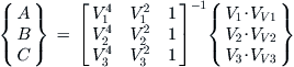
Step 4: Determine the Coefficients to the Quadratic Spline
Calculate the constants A, B, C by multiplying the inverted matrix in Step 3 with the matrix formed by column 5 in the table above:
Step 5: Extract Aerodynamic Properties
Using the constants A, B, C calculated in the previous step, extract the aerodynamic properties:
Derivation of Equations (15-124) through (15-127)
![]()
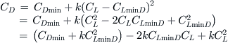
Insert the expression for CD into the ROD and expand:
Manipulate some more:
Multiply through by V to get:
![]()
where
![]()
where ![]()
We need three points (i.e. VV corresponding to a V) to determine these parameters:
Therefore:
Then, the coefficients can be found as follows:
Also note that:
![]()
QED
EXAMPLE 15-18
Consider the flight polar for a powered sailplane shown in Figure 15-74. Extract its drag characteristics, ignoring the existence of a drag bucket and assuming it can be described using the adjusted drag model.
Solution
Some properties of the aircraft that are necessary in the following calculations are:
| Gross weight: | W0 = 1876 lbf |
| Wing area: | S = 202 ft2 |
| Wing aspect ratio: | AR = 29.29 |
Step 1 through 3: The three selected points are shown in Figure 15-74 and are tabulated below:
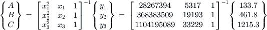
Step 4: Calculate the constants A, B, C:
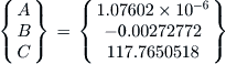
Step 5: Extract the aerodynamic properties using the constants A, B, C:
15.6.3 Step-by-step: Extracting Drag Coefficient for a Piston-Powered Propeller Aircraft
The drag coefficient of piston-powered airplanes can be extracted from typical data provided in the Pilots Operating Handbooks (POH). The accuracy is contingent upon the quality of the data provided by the corresponding manufacturer, but some manufacturers have been guilty of bolstering performance data so the actual aircraft did not meet the values in the POH. Therefore, the results should be taken with a grain of salt. Additionally, as far as piston airplanes are concerned, the hardest parameter to obtain is the propeller efficiency. An educated guess may have to be used. The methods of Chapter 14, The anatomy of the propeller, should be helpful.
Method 1: Extraction CDmin Using Cruise Performance
The following procedure is intended to illustrate how such data extraction would take place using cruise performance. The reader may have to modify the procedure for selected aircraft, although it is thought that most POH feature data of the kind shown. Here, we will illustrate the method using a data sheet for a Cirrus SR22.
Figure 15-75 shows a page from a POH for a Cirrus SR22. The same information can also be obtained from the Type Certificate Data Sheet, also in the public domain and can be downloaded from the FAA official website (www.faa.gov). The excerpt shown displays the form typically used for General Aviation aircraft.

Step 1: Determine the following parameters for the type: reference area (S) in ft2, aspect ratio (AR), rated engine power (PA) in BHP, and gross weight (W0) in lbf.
Step 2: Using the POH, extract the cruising speed and the associated altitude. Usually, these numbers are normalized to the gross weight. Typically, manufacturers present the cruising speed in KTAS, since this will make the number look larger and thus “better” in the POH. However, be alert in the unlikely event the data is provided as KIAS or KCAS. For this procedure, the airspeed in KTAS must be used.
Step 3: Determine the density of air, ρ, at the cruise altitude using Equation (16-18). Convert the airspeed in KTAS to ft/s by multiplying it by 1.688. This airspeed is V.
Step 4: Determine the Oswald efficiency and the lift-induced drag constant at the condition. For a medium AR aircraft, Equation (9-89) can be used, repeated here for convenience:
Step 5: Calculate the minimum drag coefficient from:
![]() (15-128)
(15-128)
Note that the selection of ηp can be tricky. If the propeller is a fixed-pitch “climb” propeller use a value ranging from 0.65 to 0.70. If the propeller is a fixed-pitch “cruise” propeller use a value ranging from 0.75 to 0.80. If the airplane is equipped with a constant-speed propeller, use a value ranging from 0.80 to 0.86.
Derivation of Equation (15-128)
Since thrust equals drag at this condition, we can determine the drag coefficient as follows:
![]()
Furthermore, using the simplified drag model and the lift coefficient the lift-induced drag is given by:
![]()
Inserting this into the expression for CDmin yields:
![]()
QED
EXAMPLE 15-19
Estimate the total, induced, and minimum drag coefficient for the Cirrus SR22, using the data in Figure 15-75 using the published cruising speed of 183 KTAS at 8000 ft and 78% power at ISA condition.
Solution
Step 1–2:
| Reference area | S = 144.9 ft2 |
| Aspect ratio | AR = 10.1 (using a wing span of 38.3 ft) |
| Engine power at condition | PA = 0.78 × 310 BHP = 241.8 BHP |
| Gross weight | W0 = 3400 lbf |
Cruising speed is 183 KTAS at 8000 ft.
Step 3:
Cruising speed in ft/s is V = 183 × 1.688 = 308.9 ft/s
Step 4: Both the Oswald efficiency factor and lift-induced drag constant have been calculated multiple times throughout this book. Of the two we need the latter one for this problem and it has been shown to be k = 0.04207.
Step 5: Since we don’t know the propeller efficiency we will have to guess. The propeller is a constant-speed propeller, specifically designed for the aircraft, so it is not unlikely its propeller efficiency is as high as 0.85 at this condition. The reader must remember that this is a guess so the resulting drag coefficient must be regarded with caution. Therefore, we can estimate the minimum drag coefficient for the airplane as follows:

The total drag can be estimated using the thrust relation shown in the above derivation:
And the lift-induced drag is the difference between the total and minimum drag:
![]()
Method 2: Extracting CDmin Using Climb Performance
The following procedure is intended to illustrate how such data extraction would take place using climb performance. This requires the rate-of-climb (ROC) and the associated airspeed and altitude to be determined. Ideally, this should be the best ROC, obtained at VY (the best rate-of-climb airspeed). The reason is that VY occurs at a relatively low AOA, which means less flow separation than at, say, VX (the best angle-of-climb airspeed) and, thus, closer adherence to the quadratic drag model. It is also better to use data at S-L as this will require fewer corrections.
Figure 15-75 shows a page from a POH for a Cirrus SR22. The same information can also be obtained from the Type Certificate Data Sheet, which is in the public domain and can be downloaded from the FAA official website (www.faa.gov). The excerpt shown displays the form typically used for General Aviation aircraft.
Step 1: Same as Step 1 of Method 1.
Step 2: Using the POH, extract the ROC, the associated climb airspeed, and altitude. Ideally this would be VY at S-L. Usually, these numbers are normalized to the gross weight. It is common for manufacturers to present the climb speed in KIAS. If this is the case, it must be corrected to KCAS before it is converted to KTAS, which is required for this procedure. This conversion should be implemented using the methods of Section 16, Performance – introduction.
Step 3: Determine the density of air, ρ, at the climb altitude using Equation (16-18). Ideally, this should be at S-L, in which case ρ = 0.002378 slugs/ft3. Convert the ROC in fpm to VV by dividing it by 60 seconds/minute, i.e. VV = ROC/60. Convert the airspeed in KTAS to ft/s by multiplying it by 1.688. This airspeed is V.
Step 4: Same as Step 4 of Method 1.
Step 5: Calculate the minimum drag coefficient from:
![]() (15-129)
(15-129)
Again, note that if the propeller efficiency, ηp, is not known, one must rely on engineering judgment to assess its value, and this can be tricky. Assuming the flight condition to be at VY, use a value ranging from 0.65 to 0.70 if the propeller is a fixed-pitch “climb” propeller. If the propeller is a fixed-pitch “cruise” propeller, use a value ranging from 0.55 to 0.65, and if equipped with a constant-speed propeller, use a value ranging from 0.65 to 0.70. Also note that, just like for Method 1, correcting the power to the altitude at which the aircraft is operating is crucial. For this, use the Gagg and Ferrar model of Equation (7-16).
Derivation of Equation (15-129)
Replacing the thrust, T, and drag, D, with the standard expressions yields:
![]()
Mulitplying through by W and inserting the simplified drag model and, then, the lift coefficient leads to:
![]()
Solving for the CDmin returns:
![]()
QED
EXAMPLE 15-20
Estimate the minimum drag coefficient for the Cirrus SR22, using the climb performance extraction method at VY and the following data in addition to S, k, and W from the previous example.
Solution
Step 1–2:
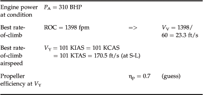
Note that if the propeller efficiency is 0.689, rather than 0.700, the CDmin will be 0.02541, which is the same as that of Method 1. This shows the importance of properly selecting the propeller efficiency.
15.6.4 Computer code 15-1: Extracting Drag Coefficient from Published Data for Piston Aircraft
The following Visual Basic for Applications routine can be used with Microsoft Excel to extract various drag-related parameters using the above method. Note that, as shown, it is only valid for aircraft with straight wings. Also, note that the power is not necessarily the rated power. For instance, the rated power for the SR22 is 310 BHP. However, at the condition used in Example 15-18, the power was only 241.8 BHP. Regardless of whether the number is due to altitude effects (see Equation (7-16)) or power setting or a combination of the two, the power at the condition must be used.
15.6.5 Step-by-step: Extracting Drag Coefficient for a Jet Aircraft
The drag coefficient of jets can be extracted from typical data published by similar means, e.g. the Pilots Operating Handbooks (POH) or Pilot’s Flight Manual (PFM), with all the limitations as before. Sometimes, a surprising amount of information can be learned from document such as Ref. [45]. The primary difficulty is that the maximum level airspeed of many jets is not limited by engine thrust, but by compressibility effects. This is denoted by the MMO or the maximum operating Mach number (maximum and operating are denoted by the subscript). As a matter of fact, the engines often have enough thrust to accelerate the aircraft beyond the MMO value and thrust must therefore be set to prevent this from taking place. Thus, different jets require different fractions of maximum thrust for operation, making the determination of their minimum drag based on cruise information that much harder.
For this reason, we will attempt to extract the minimum drag based on other kind of information – the best rate-of-climb (ROC). This important form of climb is usually presented in performance handbooks. This can be done by at least two means, based on the available information, and the assumption that the reported climb is VY and performed at max thrust and with all high-lift devices retracted.
Step 1: Using the PFM or other reliable sources, extract the best rate of climb airspeed, the associated altitude. Now the two following scenarios are possible: (1) The ROC given is not necessarily the best ROC, but has an associated airspeed presented. In this case use Method 1 in Step 7 below. (2) The ROC is not given but the airspeed for best ROC (VY). In this case use Method 2.
For jets, these numbers are not necessarily normalized to the gross weight but to some specific operational weights. If so the appropriate weight must be used throughout. Typically, manufacturers present the cruising speed in KTAS or Mach numbers. In either case, the corresponding numbers must be converted to ft/s true airspeed.
Step 2: The following parameters for the type are required based on the discussion in Step 1:
(1) Reference area (S) in ft2.
(3) Maximum total rated engine thrust (TA), in lbf.
(4) Aircraft weight (W) at condition, in lbf.
Step 3: Determine the density of air, ρ, at the cruise altitude using Equation (16-18).
Step 4: Convert Mach numbers to ft/s by calculating the speed of sound at altitude and multiplying by the Mach number, per Equation (16-30).
Convert the airspeed in KCAS to ft/s by multiplying it by 1.688 and then dividing by the square root of the density ratio, per Equation (16-33).
Step 5: Correct the rated thrust for airspeed and altitude using the Mattingly method for turbojets or turbofans in Sections 7.2.3, Turbojets, or Section 7.2.4, Turbofans.
Important: It is imperative that the thrust be corrected with respect to the altitude and airspeed, as this is much less than the rated thrust. Otherwise, erroneous results will be returned.
Step 6: Determine the Oswald efficiency at the condition using either Equation (9-90) or (9-91), repeated here for convenience:
![]() (9-90)
(9-90)
![]() (9-91)
(9-91)
Of these, the author considers Equation (9-85) more suitable for typical modern transportation jets. Then calculate the lift-induced drag constant:
![]()
Step 7a – Method 1 (airspeed other than VY and the associated ROC are known):
Calculate the minimum drag coefficient from (remember that (1) V must be in ft/s true airspeed and may or may not be VY and (2) the ROC must correspond to V and be in ft/min):
Step 7b – Method 2 (the best rate-of-climb and associated airspeed are known):
Calculate the minimum drag coefficient from (remember that VY must be in ft/s true airspeed):


15.6.6 Determining Drag Characteristics from Wind Tunnel Data
Standard wind tunnel testing yields a number of static force and moment coefficients such as CD, CL, CY, Cl, Cm, and Cn. For this section the focus is on the first two: the lift and drag coefficients. A conventional AOA sweep (or alpha-sweep as it is most often called) consists of changing the AOA from a given minimum value (e.g. −5°) to a maximum value (e.g. +20°), perhaps 1° at a time. Therefore, the sweep returns a listing of the coefficients as a function of α. For standard aircraft that do not generate a noticeable drag bucket, the relationship between CL and CD can then be obtained using a quadratic least-squares curve-fit, which returns a polynomial of the form CD = A·CL2 + B·CL + C. The coefficients of this polynomial can be used to extract the coefficient CDmin, CLminD, and the Oswald span efficiency factor, e, provided the airplane’s AR has been established. If so, it can then be shown that these parameters are related to the constants of the curve-fit polynomial as follows:
![]() (15-132)
(15-132)
![]() (15-133)
(15-133)
![]() (15-134)
(15-134)
Derivation of Equations (15-132) through (15-134)
Begin by equating the two forms of the drag coefficients: the quadratic curve-fit and the adjusted drag model of Equation (15-6):
![]()
Expand and sort coefficients based on their dependency on CL2 and CL:
![]()
By observation we see that A, B, and C are related to the constants of the adjusted drag polar as follows:
![]() (i)
(i)
![]() (ii)
(ii)
![]() (iii)
(iii)
From Equation (i) we get:
![]()
Using this result with Equation (ii) we get:
![]()
Using the two previous results with Equation (iii) we get:
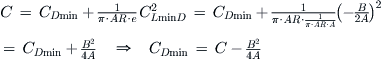
QED
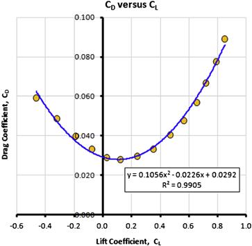
EXAMPLE 15-21
The data from a wind tunnel test of a complete aircraft configuration is given in the following table:

Determine the parameters CDmin, CLminD, and the Oswald span efficiency factor, e, using a quadratic least-squares curve-fit to the data of the form CD = A·CL2 + B·CL + C, if the aspect ratio, AR, = 6.
Solution
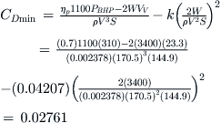
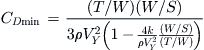
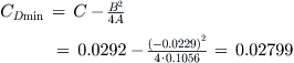
One way to obtain the curve-fit is to use commercial spreadsheet software like Microsoft Excel, enter the data and plot using a scatter graph. Then, the user can select the curve and add a trendline with the associated equation and correlation coefficient display. This is shown in Figure 15-76. The resulting curve-fit shows the polynomial constants are given by A = 0.1056, B = −0.0226, and C = 0.0292. Then the drag parameters can be determined as follows:
![]()
![]()
15.7 Additional Information – Drag of Selected Aircraft
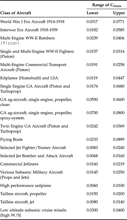
15.7.1 General Range of Subsonic Minimum Drag Coefficients
Table 15-17 shows expected ranges of values of the subsonic minimum drag coefficient for several classes of aircraft. These numbers do not bracket all possible aircraft configurations – i.e. there may be specific aircraft that are outside the range shown. However, most aircraft will be inside the lower and upper limits of the range.
15.7.2 Drag of Various Aircraft by Class
Table 15-18 lists selected drag related figures for a number of aircraft of different classes. Some of these are displayed in Figure 15-31. The data was gathered from a number of sources. Note that some of the data was retrieved from graphs using “careful eyeballing” and should be regarded with care.
TABLE 15-18
Drag Characteristics of Selected Aircraft
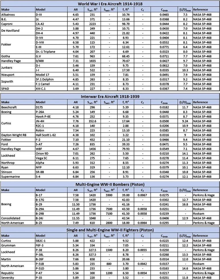
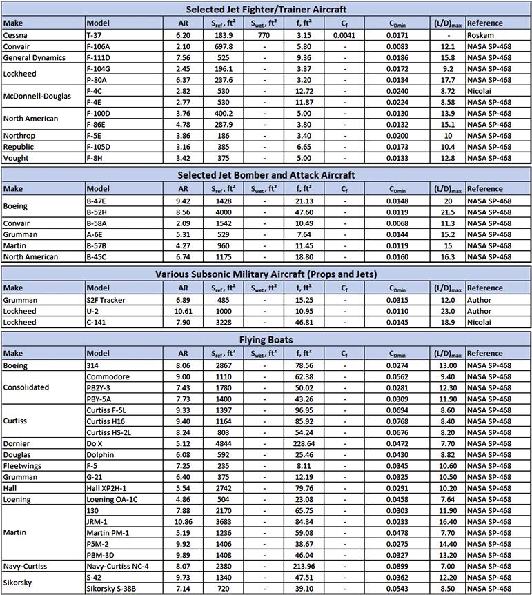
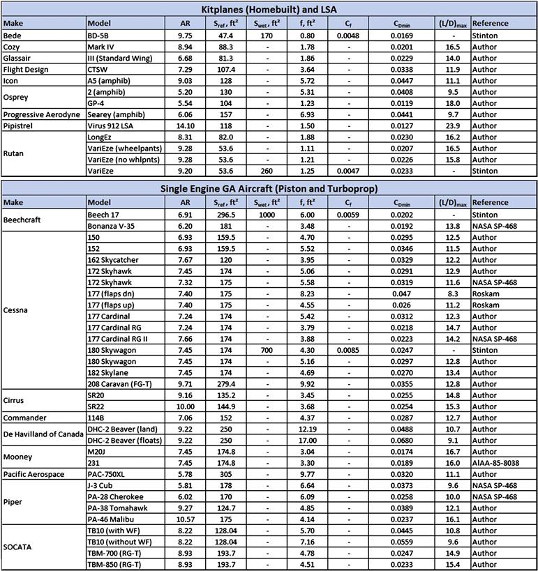

RG = retractable gear, FG = fixed gear, T = turboprop, WF = wheel fairings, f = equivalent flat plate area = CDmin × Sref.
When estimating the drag of a new aircraft design, it is strongly recommended that the designer compares his own results to that of the aircraft in the tables below that most similarly resembles the new aircraft. This can help flag a possible over- or underestimation.
The numbers come from a variety of sources; Perkins and Hage [24], Stinton [46], Roskam [47], Nicolai [28], NASA SP-468 [48], NASA CR-114494 [49], and the author’s own estimates. The author’s estimations utilize Method 1 of Section 15.6.3, Step-by-step: Extracting drag coefficient for a piston-powered propeller aircraft, and 15.6.5, Step-by-step: Extracting drag coefficient for a jet aircraft, utilizing performance data from the corresponding aircraft’s Pilots Operating Handbook (POH) or other reliable sources. The LDmax estimated by the author for propeller aircraft assumes no additional drag due to windmilling or stopped propellers. Refer to Section 15.5.13, Drag of windmilling and stopped propellers, for methods on how to account for this drag. Windmilling propellers can easily increase the minimum drag coefficient by 150 drag counts or more. Additionally, although expected, there is no guarantee the manufacturer has not bolstered performance values in the POH. For this reason, treat all drag data with caution.
Exercises
(1) Estimate the skin friction coefficient for an airfoil whose chord is 5.25 ft at 25,000 ft and 250 KTAS airspeed on a day on which the outside air temperature is 30 °F warmer than a standard day. Do this using the following assumptions:
(a) fully laminar boundary layer
(b) fully turbulent boundary layer assuming incompressible flow,
(c) fully turbulent boundary layer assuming compressible flow,
(d) mixed boundary layer for which the transition on the upper surface occurs at chord station 1.3 ft and at 65% chord on the lower surface.
Answer: (a) 0.0005037, (b) 0.003186, (c) 0.003139, (d) 0.002119.
(2) An aircraft has a drag polar given by ![]() . Determine the CL where LDmax occurs and the magnitude of the LDmax. (Hint:
. Determine the CL where LDmax occurs and the magnitude of the LDmax. (Hint: ![]() )Answer: CL where LDmax occurs is 0.8549, LDmax is 11.71.
)Answer: CL where LDmax occurs is 0.8549, LDmax is 11.71.
(3) Consider the wing shown in Figure 15-77 and for which the representative skin friction coefficients for each of the three wing segments have already been calculated. Note that all data required for geometric evaluation is given in the figure. Assume a wetted area booster factor of 1.07. Determine the total skin friction coefficient and total skin friction drag coefficient for the wing half. Estimate the total skin friction drag force of both wing halves at airspeed of 150 KTAS at S-L on a standard day.
Answer: Cf = 0.005045, CDf = 0.01080, Df = 183 lbf.
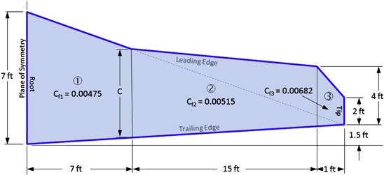
(4) An airplane has two dissimilar airfoils at the root and tip of the wing (see Figure 15-78). Important dimensions to use are:
b = 18 ft, CR = 3 ft, CT = 2 ft and Sref = 45 ft2.
The root airfoil is a NLF airfoil capable of sustaining 55% laminar flow on the upper surface and 35% on the lower. The tip airfoil is a turbulent flow airfoil that sustains laminar flow to 15% on the upper and lower surfaces.
If the airplane is cruising at 100 KTAS at S-L ISA, determine the skin friction drag coefficient and force acting on the wing due to the mixed laminar and turbulent BL regions. Compare to a wing with fully laminar or fully turbulent BL.
Answer: Cf = 0.003115, CDf = 0.006230, Df = 9.5 lbf.
(5) Extract the total, induced, and minimum drag coefficient for the single-piston-engine propeller-powered Cessna 172N Skyhawk II using the data below obtained from its POH. Hint: use Equation (9-89) to estimate the Oswald span efficiency and assume a propeller efficiency of 0.80.
Wing span is 36.08 ft, wing area is 174 ft2, cruising speed at 8000 ft and 75% power is 122 KTAS. Engine is a Lycoming O-320 rated at 160 BHP at S-L. Gross weight is 2300 lbf.
Answer: CD = 0.03714, CDmin = 0.03141, CDi = 0.005728.
(6) Extract the CLminD, CDmin, and e for the wind tunnel data (points) shown in the table and graph of Figure 15-79. The solid line is a least-squares curve-fit whose constants and correlation coefficients are shown in the legend. The AR for the airplane being tested is 6.

Answer: CLminD = 0.2574, CDmin = 0.0252, e = 0.5584.
References
1. Levy David. AIAA CFD Drag Prediction Workshop, Data Summary and Comparison. June 9–10, 2001.
2. In: http://aaac.larc.nasa.gov/tsab/cfdlarc/aiaa-dpw/.
3. Hoerner Sighard F. Fluid-Dynamic Drag. L. Hoerner 1965.
4. Schlichting Hermann. Boundary Layer Theory. English ed. Pergamon Press 1955; p. 16.
5. Young AD. Boundary Layers. AIAA Education Series 1989.
6. Schetz Joseph A, Rodney D W Bowersox. Boundary Layer Analysis. AIAA Education Series 2011.
7. Roskam Jan, Chuan-Tau Edward Lan. Airplane Aerodynamics and Performance. DARcorporation 1997; Equations (2.90) and (2.91).
8. Hoak DE. USAF Stability and Control DATCOM. Flight Control Division, Air Force Flight Dynamics Laboratory 1978; Section 4.1.5.1.
9. NACA-TR-572. Determination of the Characteristics of Tapered Wings. Anderson, Raymond F. 1936.
10. R.&M No 1226, The Characteristics of a Tapered and Twisted Wing with Sweep-Back. Aeronautical Research Council, Glauert, H., and S. B. Gates 1929.
11. Hueber J. Die Aerodynamischen Eigenschaften von Doppel-Trapezförmigen Tragflügeln. Z.F.M. 13 May 1933; pp. 249–251; 29 May 1933, pp. 269–272.
12. NASA SP-2005-4539. Innovation In Flight: Research of the Nasa Langley Research Center on Revolutionary Advanced Concepts for Aeronautics. Chambers, Joseph R. 2005; pp. 123–161.
13. Braslow Albert L. A History of Suction-Type Laminar-Flow Control with Emphasis on Flight Research. Monographs in Aerospace History Number 13, NASA 1999.
14. Marshall Laurie A. Boundary-Layer Transition Results From the F-16XL-2 Supersonic Laminar Flow Control Experiment. NASA TM-1999–209013 1999.
15. van de Wal HJB. Design of a Wing with Boundary Layer Suction. M.Sc. Thesis Delft University of Technology 2010.
16. Wortman Andrzej. Reduction of Fuselage Form Drag by Vortex Flows. Journal of Aircraft,. May–June 1999;vol. 36.
17. Kentfield JAC. Drag Reduction by Means of Controlled Separated Flows. AIAA-1985-1800-493 1985.
18. NASA TM-77785 Profile Design for Wings and Propellers. Quast, A., and K. H. Horstmann Nov. 1984.
19. Peigin S, Epstein B. Aerodynamic Optimization of Essentially Three-Dimensional Shapes for Wing-Body Fairing. AIAA Journal,. July 2008;vol. 46.
20. NACA R-116 Applications of Modern Hydrodynamics to Aeronautics. Prandtl, Ludwig 1923.
21. Whitford Ray. Design for Air Combat. Jane’s 1987.
22. Torenbeek Egbert. Synthesis of Subsonic Aircraft Design. 3rd ed. Delft University Press 1986; p. 499.
23. Roskam Jan. Methods for Estimating Drag Polars of Subsonic Airplanes. 4th printing 1984.
24. Perkins Courtland D, Robert EHage. Airplane Performance, Stability, and Control. John Wiley & Sons 1949.
25. Raymer Daniel. Aircraft Design: A Conceptual Approach. 4th ed. AIAA Education Series 2006.
26. Torenbeek Egbert. Synthesis of Subsonic Aircraft Design. 3rd ed. Delft University Press 1986.
27. Shevell Richard S. Fundamentals of Flight. Prentice Hall 1983.
28. Nicolai Leland. Fundamentals of Aircraft Design. 2nd ed. 1984.
29. Jenkinson Lloyd R. Civil Jet Aircraft Design. Arnold 1999.
30. NACA WR-L-489. Drag Analysis of Single-Engine Military Airplanes Tested in the NACA Full-Scale Wind Tunnel Dearborn. C. H., and Abe Silverstein 1940.
31. McCormick Barnes W. Aerodynamics, Aeronautics, and Flight Mechanics. John Wiley & Sons 1979.
32. NACA R-485 The Drag of Airplane Wheels, Wheel Fairings, and Landing Gears – I. Herrnstein, William H., and David Biermann 1935.
33. Austyn-Mair W, Birdsall David L. Aircraft Performance. Cambridge, England: Cambridge University Press; 1992; p. 124. Method is based on ESDU 79015, Undercarriage Drag Prediction Methods.
34. Jenkinson Lloyd R, Simpkin Paul, Rhodes Darren. Civil Jet Aircraft Design. AIAA Education Series 1999.
35. NACA WR-L-238 Wind-Tunnel Tests of Four Full-Scale Seaplane Floats. Conway, Robert N., and Julian D. Maynard 1943.
36. NACA TN-716 Hydrodynamic and Aerodynamic Tests of a Family of Models of Seaplane Floats with Varying Angles of Dead Rise. Parkinson, John B., Roland E. Olson, and Rufus O. House 1939.
37. Young AD. The Aerodynamic Characteristics of Flaps. R.&M. No. 2622, British A. R. C. 1947.
38. Corke Thomas C. Design of Aircraft. Prentice-Hall 2003.
39. Linden F, Robert Van Der. The Boeing 247: The First Modern Airliner. University of Washington Press 1991.
40. NACA WR-L-462 Investigation of Drag and Pressure Distribution of Windshields at High Speeds. Wright, Ray M. 1942.
41. NACA R-464 Negative Thrust and Torque Characteristics of an Adjustable-Pitch Metal Propeller. Hartman, Edwin P. 1934.
42. NACA WR-L-502 High-Speed Wind-Tunnel Tests of Gun Openings in the Nose of the Fuselage of a 1/4-Scale Model. Fedziuk, Henry A. 1942.
43. NACA WR-L-292 Effects of Simulated Ice Formation on the Aerodynamic Characteristics of an Airfoil. Gulick, Beverly G. 1938.
44. NACA TN-2962 Effect of Ice and Frost Formations on Drag of NACA 65(sub 1) -212 Airfoil for Various Modes of Thermal Ice Protection. Gray, V. H., and U. H. Von Glahn 1953.
45. Jane’s All the World’s Aircraft. Various editors. Janes Yearbooks, various years.
46. Stinton Darrol. The Design of the Aeroplane. Collins 1983.
47. Roskam Jan. Airplane Design. Part VI. DARcorporation 2000.
48. Loftin Jr Laurence K. Quest for Performance; The Evolution of Modern Aircraft. NASA SP-468 1985.
49. Hanke CR, Nordwall DR. The Simulation of a Jumbo Jet Transport Aircraft, Volume 2: Modeling Data. NASA-CR-114494 1970.
50. NACA TN-525 The Aerodynamic Drag of Flying-Boat Hull Model as Measured in the NACA 20-foot Wind Tunnel I. Hartman, Edwin P. 1935.
1Then again, many would argue that novices shouldn’t be estimating drag in the first place.
2AIAA is the American Institute of Aeronautics and Astronautics.
3Using a value of k higher than 62 (e.g. 200, 400, or higher) will effectively make the polar flatter and flatter.
4Note that some authors, e.g. Stinton, describe diameter as being (b√2), but most other texts use the presentation shown.
5Eiffel is considered by many to be the father of aerodynamics, while others place the honor on Cayley.