
Chapter 12. A 2D and 3D Transformation Library for Graphics
12.1. Introduction
The ideas of the previous chapters can be nicely condensed into an implementation—a collection of cooperating classes that help to maintain the point/vector distinction, the distinction between a transformation T that acts on points and the associated transformations of vectors and covectors, and some of the other routine computations that are often done in graphics.
This chapter can be regarded as an instance of the Implementation principle: that if you understand a mathematical idea well enough, you can implement it in code, and thereafter be insulated from the need for further understanding.
The book’s website has such an implementation in C#, starting with the predefined Point, Vector, Point3D, and Vector3D WPF classes that you’ve already seen. You should download the implementation and look at it as you read this chapter.
The implementation depends on a matrix library—one capable of inverting matrices, solving linear systems, multiplying matrices, etc. We’ve chosen to import the MathNet.Numerics.LinearAlgebra library [Mat], but if you prefer another one, it should be easy to substitute, as our use of the library is highly localized.
In most of the classes there are procedures that can fail under certain circumstances. For instance, if you ask for a linear transformation that sends v1 to w1 ≠ 0, and also sends v1 to 2w1, there is no satisfactory answer. All such failures amount to some matrix being noninvertible. We raise exceptions in these situations. They are discussed in the code and its documentation, but not in this chapter.
The approach taken in our implementation is not the only one possible. Our approach depends on transformations as the primitive notion, but it’s quite possible and reasonable to think instead of coordinate systems as the fundamental entity. Just as in Chapter 10 we discussed the interpretation of a linear transformation as a change of coordinates, you can approach much of graphics with this point of view. You end up having coordinate frames for vector spaces (for a 2D space, you have two independent vectors; for a 3D space, you have three independent vectors), for affine spaces (typically a coordinate frame for a 2D affine space consists of three points, from which you determine barycentric coordinates, but you can also build a frame from one point and two vectors), and for projective spaces (where in 2D, a projective frame is represented by four points in “general position,” which we’ll discuss shortly). This coordinate frame approach is taken by Mann et al. [MLD97].
12.2. Points and Vectors
The predefined Point and Vector classes in WPF already implement the main ideas we’ve discussed (for two dimensions): There are operators defined so that you can add one Point and one Vector to get a new Point, but there is no operator for adding two Points, for instance. Certain convenience operations have been included, like the dot product of Vectors.
There are idiosyncrasies in the design of the classes, however. The two coordinates of a point P are P.X and P.Y; there’s no way to refer to them as elements of an array of length 2, nor even a predefined “cast” operation to convert to a double[2]. There is, however, a predefined CrossProduct operation for Vectors, which treats the vectors as lying in the xy-plane of 3-space, computes the 3D cross product (which always points along the z-axis), and returns the z-component of the resultant vector. In deference to the convenience of having data types that work well with the remainder of WPF, we’ve ignored these idiosyncrasies and simply used the parts of the Point and Vector classes (and their 3D analogs) that we like. We’ve also added some geometric functions to our LIN_ALG namespace (in which all the transformation classes reside) to compute things like the two-dimensional cross product of one vector.
12.3. Transformations
While WPF also has a class called Matrix, its peculiarities made it unsuitable for our use. Furthermore, we wanted to build a library in which the fundamental idea was that of a transformation rather than the matrix used to represent it. We therefore define four classes.
• MatrixTransformation2: A parent class for linear, affine, and projective transformations. Since all three can be represented by 3 × 3 matrices, a MatrixTransformation holds a 3 × 3 matrix and provides certain support procedures to multiply and invert such matrices.
• LinearTransformation2: A transformation that takes Vectors to Vectors.
• AffineTransformation2: A transformation that can operate on both Points and Vectors.
• ProjectiveTransformation2: A transformation that operates on Points in their homogeneous representation and includes a division by the last coordinate after the matrix multiplication.
(There are four corresponding classes for transformations in 3D.)
In each case, we’ve defined composition of transformations by overloading the * operator, and the application of a transformation to a Point or Vector by overloading the * operator again. To translate a point and then rotate it by π/6, we could write
1 Point P = new Point(...);
2 AffineTransformation2 T = AffineTransformation2.Translate(Vector(3,1));
3 AffineTransformation2 S = AffineTransformation2.RotateXY(Math.PI/6);
4 Point Q = (S * T) * P;
If we were planning to operate on many points with this composed transformation, we’d precompute the composed transformation and instead write
1 ...
2 AffineTransformation2 T2 = (S * T);
3 Point Q = T2 * P;
12.3.1. Efficiency
Applying a transformation to a point or vector involves some memory allocation, a method invocation, and a matrix multiplication. If you simply stored the matrix yourself, you could avoid most of this cost. And since graphics programs end up applying lots of transformations to lots of points and vectors, you might think that doing it yourself is the best possible approach. If you’re writing a program that will be doing real-time graphics on a processor where computation is a real bottleneck (e.g., a game that runs on a battery-powered device), it may well be. But as a student of computer graphics, you’re likely to write a lot of programs that get run just a few times. The great “cost” in your programs is your time as a developer. Using a high-level approach can help reduce bugs and even increase efficiency, as you notice ways to restructure your code that would be difficult to see if you were looking at every detail all the time. A profiler can help you to determine exactly where in your code it’s worth the trouble of working with a low-level construct rather than a high-level one.
Nonetheless, there are places where one can get a certain amount of efficiency at no cost. For instance, the LinearTransformation2 class uses a 3 × 3 matrix to represent a transformation, but that matrix always has the form
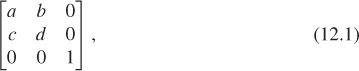
so it’s much easier to invert than a general 3 × 3 matrix (we just invert the upper-left 2 × 2 matrix); in the same way, multiplying two of these is much less work than multiplying two 3 × 3 matrices (we just multiply the upper-left 2 × 2 matrices). By overriding the MatrixTransform2 methods for inversion and multiplication, we get a large efficiency improvement.
Without looking at the code, consider whether you can find a more efficient way to invert an affine transformation on R2 than by inverting its 3 × 3 matrix. Hint: The bottom row of the matrix is always [0 0 1].
12.4. Specification of Transformations
For each kind of transformation, the default constructor generates the identity transformation. (The constructor for MatrixTransformation2 is protected, as only the derived classes are supposed to ever create a MatrixTransformation.) In general, though, transformations are constructed by static methods with mnemonic names. For the AffineTransformation2 class, for instance, there are eight static methods (all public static AffineTransform2) that construct transformations.
1 RotateXY(double angle)
2 Translate(Vector v)
3 Translate(Point p, Point q)
4 AxisScale(double x_amount, double y_amount)
5 RotateAboutPoint(Point p, double angle)
6 PointsToPoints(Point p1, Point p2, Point p3, Point q1, Point q2, Point q3)
7 PointAndVectorsToPointAndVectors(Point p1, Vector v1, Vector v2,
8 Point q1, Vector w1, Vector w2)
9 PointsAndVectorToPointsAndVector(Point p1, Point p2, Vector v1,
10 Point q1, Point q2, Vector w1)
The naming convention is straightforward: “From” comes before “to” so that
Translate(Point p, Point q)
creates a translation that sends p to q, and within a collection of arguments, points come before vectors so that in
PointAndVectorsToPointAndVectors
the point p1 is sent to the point q1, the vector v1 is sent to the vector w1, and the vector v2 is sent to the vector w2. The method name tells you that there is one point and more than one vector; since an affine transformation of the plane is determined by its values on three points, or one point and two vectors, or two points and one vector, you know that the arguments must be one point and two vectors.
Methods that produce particular familiar transformations—translations, rotations, axis-aligned scales—have names indicating these. While the names are sometimes cumbersome, they are also expressive; it’s easy to understand code that uses them.
12.5. Implementation
Most of the transformations are easy to implement. For instance, we first implemented the
method for AffineTransformation2; once we’d done this, the PointsToPoints method was straightforward:
1 public static AffineTransform2 PointsToPoints(
2 Point p1, Point p2, Point p3,
3 Point q1, Point q2, Point q3)
4 {
5 Vector v1 = p2 - p1;
6 Vector v2 = p3 - p1;
7 Vector w1 = q2 - q1;
8 Vector w2 = q3 - q1;
9 return AffineTransform2.PointAndVectorsToPointAndVectors(p1, v1, v2, q1, w1, w2);
10 }
The PointAndVectorsToPointAndVectors code is implemented in a relatively straightforward way: We know that the vectors v1 and v2 must be sent to the vectors w1 and w2; in terms of the 3 × 3 matrix, that means that the upper-left corner must be the 2 × 2 matrix that effects this transformation of 2-space. So we invoke the LinearTransformation2 method VectorsToVectors to produce the transformation. Unfortunately, the resultant transformation does not send p1 to q1 in general. To ensure this, we precede this vector transform with a translation that takes p1 to the origin (the translation has no effect on vectors, of course); we then perform the linear transformation; we then follow this with a transformation that takes the origin to q1. The net result is that p1 is sent to q1, and the vectors are transformed as required.
This approach relies on the VectorsToVectors method for LinearTrans-formation2. Writing that is straightforward: We place the vectors v1 and v2 in the first two columns of a 3 × 3 matrix, with a 1 in the lower right. This transformation T sends e1 to v1 and e2 to v2. Similarly, we can use the w’s to build a transformation S that sends e1 to w1 and e2 to w2. The composition T ο S–1 sends v1 to e1 to w1, and similarly for v2, and hence solves our problem.
12.5.1. Projective Transformations
The only really subtle implementation problem is the PointsToPoints method for ProjectiveTransformation2. Explaining this code requires a bit of mathematics, but it’s all mathematics that we’ve seen before in various forms.
We’re given four points P1, P2, P3, and P4 in the Euclidean plane, and we are to find a projective transformation that sends them to the four points Q1, Q2, Q3, and Q4 of the Euclidean plane.
Before we go any further, we should mention a limitation. When we described the VectorsToVectors method of LinearTransformation2, we promised to send v1 and v2 to w1 and w2, but there was, in fact, a constraint. If v1 = 0 and w1 ≠ 0, there’s no linear transformation that accomplishes this. In fact, if v1 is a multiple of v2, in general there’s no linear transformation that solves the problem (except in the very special case where w1 is the same multiple of w2, in which case there are an infinite number of solutions). The implicit constraint was that v1 and v2 must be linearly independent for our solution to work (or for the general problem to have a solution). In the case of PointsToPoints, we require something similar: The points Pi (i = 1, ..., 4) must be in general position, which means that (a) no two of them can be the same, and (b) none of them can lie on the line determined by two others (see Figure 12.1). In more familiar terms, this is equivalent to saying (a) that P1, P2, and P3 form a nondegenerate triangle, and (b) that the barycentric coordinates of P4 with respect to P1, P2, and P3 are all nonzero. We’ll further require that the Qis are similarly in general position.1
1. This latter condition is overly stringent, but it simplifies the analysis somewhat.
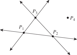
Figure 12.1: The four points are in general position, because (a) none of them lies on a line passing through another pair or (b) the first three form a nondegenerate triangle, and the fourth is not on the extensions of any of the sides of this triangle. These two descriptions are equivalent.
Returning to the main problem of sending the Ps to the Qs, when we express the points Pi and Qi as elements of 3-space, we append a 1 to each of them to make it a vector whose tip lies in the w = 1 plane. We’ll call these vectors p1, p2, etc. Our problem can then be expressed by saying that we seek a 3 × 3 matrix M with the property that
for some four nonzero numbers α, β, γ, and δ (because, for instance, αq1, when we divide through by the last coordinate, will become q1). The problem is that we do not know the values of the multipliers.
This problem, as stated, is too messy. If there were no multipliers, we’d be looking for a 3 × 3 matrix with Mpi = qi (i = 1, ..., 4). We can only solve such problems for three vectors at a time, not four. Thus, the multipliers are essential—without them, there’d be no solution at all in general. But they also complicate matters: We’re looking for the nine entries of the matrix, and the four multipliers, which makes 13 unknowns. But we have four equations, each of which has three components, so we have 12 equations and 13 unknowns, a large underdetermined system. It’s easy to see why the system is underdetermined, though: If we found a solution (M, α, β, γ, δ), then we could double everything and get another equally good solution (2M,2α,2β,2γ,2δ) to Equations 12.2–12.5.
So the first step is to make the solution unique by declaring that we’re looking for a solution with δ = 1. This gives 13 equations in 13 unknowns. We could just solve this linear system. But there’s a simpler approach that involves much less computation in this 3 × 3 case, and even greater savings in the 4 × 4 case.
Show that fixing δ = 1 is reasonable by showing that if there is any solution to Equations 12.2–12.5, then there is a solution with δ = 1. In particular, explain why any solution must have δ ≠ 0.
We’ll follow the pattern established in Chapter 10 in simplifying the problem. To send the p’s to the q’s, we’ll instead find a way to send four standard vectors to the q’s, and the same four vectors to the p’s, and then compose one of these transformations with the inverse of the other. The four standard vectors we’ll use are e1, e2, e3, and u = e1 + e2 + e3. We’ll start by finding a transformation that sends these to multiples of q1, q2, q3, and q4, respectively.
Step 1: The matrix whose columns are q1, q2, and q3 sends e1 to q1, e2 to q2, and e3 to q3. Unfortunately, it does not necessarily send u to q4; instead, it sends u = e1 + e2 + e3 to q1 + q2 + q3, that is, the sum of the columns. If we scale up each column by a different factor, the resultant matrix will still send ei to a multiple of qi for i = 1, 2, 3, but it will send u to a sum of multiples of the q’s. We therefore, as a first step, write q4 as a linear combination of q1, q2, q3,
which is exactly the same thing as writing Q4 in barycentric coordinates with respect to Q1, Q2, and Q3. Note that because of the general position assumption, α, β, and γ are all nonzero.
In terms of code, to find α, β, and γ we build a matrix2 Q = [q1; q2; q3] and let
2. Recall that semicolons indicate that the items listed are the columns of the matrix.
Now consider the matrix
It’s straightforward to verify that it sends ei to a multiple of qi for i = 1, 2, 3, and it sends u to the sum of its columns, which is, by Equation 12.7, exactly q4.
Step 2: Repeating this process, we can find a matrix transformation with matrix B sending e1, e2, e3, u to multiples of p1, p2, p3, p4.
Step 3: The matrix AB–1 then sends the p’s to multiples of the corresponding q’s.
Note that in solving this problem we solved a 3 × 3 system of equations and inverted a 3 × 3 matrix—which required far less computation than solving a 13 × 13 system of equations.
Explain why the matrix B = [α′p1 β′p2 γ′p3], where α′, β′, γ′ are the barycentric coordinates of P4 with respect to P1, P2, and P3, is invertible. Hint: Write B = PS, where S is diagonal and P has p1, p2, p3 as columns. Now apply the general-position assumption about the points Pi(i = 1, ..., 4).
12.6. Three Dimensions
The 3D portion of the library is completely analogous to the 2D one, except that rotations are somewhat more complicated. To implement rotation about an arbitrary vector, we use Rodrigues’ formula; to implement rotation about an arbitrary ray (specified by a point and direction), we translate the point to the origin, rotate about the vector, and translate back. The projective PointsToPoints method uses the same general approach that we used in two dimensions, replacing the solution of 21 simultaneous equations with a solution of four simultaneous equations and a 4 × 4 matrix inversion.
12.7. Associated Transformations
When we have an affine transformation T on Euclidean space, we’ve said that we can transform either points or vectors, and we’ve incorporated this into our code. For an affine transformation, we’ve also seen how to transform covectors; in the code, we’ve defined a Covector structure (which is very similar to the Vector structure in the sense of storing an array of doubles). And for affine transformations, there’s an associated transformation, T.NormalMap, of covectors. We’ve bowed to convention here in calling this the “normal map” rather than the “covector map,” since its use in graphics is almost entirely restricted to normal (co) vectors to triangles.
For a projective transformation, the associated map on vectors typically varies from point to point. In Figure 10.24, for instance, the top and bottom edges of the small square in the domain may be regarded as two identical vectors; after transformation, these vectors are no longer parallel. The associated map of vectors transformed them differently because they were based at different points. Thus, the associated vector transformation takes both a point and a vector as arguments. The details, and detailed rationale, are presented in a web addendum. The covector transform (for a projective transformation) similarly depends on the point of application.
One consequence of the point dependence for the vector and covector transformations of a projective transformation is that many operations—particularly those involving dot products of vectors, like computing how much light reflects from a surface—are best performed before the projective transformation near the end of the rendering pipeline.
12.8. Other Structures
Depending on how you plan to use the linear algebra library, it might make sense to create classes to represent other common geometric entities like rays, lines, planes in 3-space, ellipses, and ellipsoids (which are transformed to ellipses and ellipsoids, respectively, by nondegenerate linear and affine maps). A ray, for instance, might be represented by a Point and a direction Vector. It’s then natural either to define
public static Ray operator*(AffineTransformation2 T, Ray r)
or to include in the AffineTransformation2 class a method like
public Ray RayTransform(Ray r)
A good implementation would transform the ray’s Point by T, and would transform its direction Vector and normalize the result, because many computations on rays are easier when their directions are expressed as unit vectors.
12.9. Other Approaches
We mentioned that there are other approaches to encapsulating the various transformation operations needed in graphics, including basing them on coordinate frames rather than linear transformations.
There’s a particularly efficient way to create a restricted transformation library in the case that we only want to describe rigid transformations of objects. This eliminates all scaling—both uniform and nonuniform—and all nonaffine projective transformations. Thus, every transformation is simply a translation, rotation, or combination of the two. There are two advantages of considering only such transformations.
• There are no “degeneracies.” In the case of the PointsToPoints transformations we discussed earlier, there was a possibility of failure if the starting points were not in general position. No such problem arises here.
• When we need to invert such a rigid transformation, no matrix inversion procedure is needed, because the inverse of a rotation matrix A is its transpose AT.
There are disadvantages as well.
• We can no longer easily use a PointsToPoints specification for a transformation. The pairwise distances of the starting points must exactly match those of the target points, because a rigid transformation preserves distances between points. It’s impractical to try to specify target points with this property, even when the source points are (0, 0), (1, 0), and (0, 1), for instance.
• We cannot make larger or smaller instances of objects in a scene using this design. (A typical solution is to provide a method for reading objects from a file with a scale factor so that you create a large sphere by reading a standard sphere with a scale factor of 6.0, for instance.)
G3D, a package we’ll use in Chapter 32 for the implementation of two renderers, uses the rigid-motion approach. It contains a class CFrame (for “coordinate frame”); the standard instance of this is the standard coordinate frame based at the origin. The model for the scene in Figure 12.2 involves quite a lot of code, most of which describes material properties, etc. The essence of the geometric part of the modeling3 is given in Listing 12.1, from which we’ve removed all modeling of light sources and materials.
3. The camera is specified elsewhere in the program.
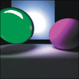
Listing 12.1: Modeling a simple scene.
1 void World::loadWorld1() {
2 modeling of lights omitted
3 // A sphere, slightly to right, shiny and red.
4 addSphere(Point3(1.00f, 1.0f, -3.0f), 1.0f, material specification );
5 // LEFT sphere
6 addTransparentSphere(Point3(-0.95f, 0.7f, -3.0f), 0.7f, material specifications );
7
8 // And a ground plane...
9 addSquare(4.0, Point3(0.0f, -0.2f, -2.0f),
10 Vector3(1.0f, 0.0f, 0.0f), Vector3(0.0f, 1.0f, 0.0f), material specifications );
11
12 // And a back plane...
13 addSquare(4.0, Point3(0.0f, 2.0f, -4.00f),
14 Vector3(1.0f, 0.0f, 0.0f), Vector3(0.0f, 0.0f, 1.0f), material specifications );
15 ...
16 }
A sphere is specified by its center point and radius; a square by its edge length, center point, a vector aligned with one axis of the square, and the normal vector to the square. These two vectors, as specified, must be perpendicular, or the code will fail. The code for adding a sphere or square to the scene is given in Listings 12.2 and 12.3.
Listing 12.2: The shape-adding methods.
1 void World::addTransparentSphere(const Point3& center, float radius,
2 material parameters ){
3 ArticulatedModel::Ref sphere =
4 ArticulatedModel::fromFile(System::findDataFile("sphere.ifs"), radius);
5 lots of material specification omitted
6 insert(sphere, CFrame::fromXYZYPRDegrees(center.x, center.y, center.z, 0));
7 }
8
9 void World::addSquare(float edgeLength, const Point3& center, const Vector3&
10 axisTangent, const Vector3& normal, const Material::Specification& material){
11 ArticulatedModel::Ref square = ArticulatedModel::fromFile(
12 System::findDataFile("squarex8.ifs"), edgeLength);
13
14 material specification code omitted
15
16 Vector3 uNormal = normal / normal.length();
17 Vector3 firstTangent(axisTangent / axisTangent.length());
18 Vector3 secondTangent(uNormal.cross(firstTangent));
19
20 Matrix3 rotmat(
21 firstTangent.x, secondTangent.x, uNormal.x,
22 firstTangent.y, secondTangent.y, uNormal.y,
23 firstTangent.z, secondTangent.z, uNormal.z);
24
25 CoordinateFrame cFrame(rotmat, center);
26 insert(square, cFrame);
27 }
Listing 12.3: The methods for inserting a shape into the scene.
1 void World::insert(const ArticulatedModel::Ref& model, const CFrame& frame) {
2 Array<Surface::Ref> posed;
3 model->pose(posed, frame);
4 for (int i = 0; i < posed.size(); ++i) {
5 insert(posed[i]);
6 m_surfaceArray.append(posed[i]);
7 Tri::getTris(posed[i], m_triArray, CFrame());
8 }
9 }
As you can see, the sphere-adding code reads the model from a file and accepts a scaling parameter that says how much to scale the model up or down. The returned object represents a shape; its coordinates are assumed to be in the standard coordinate frame. This shape is then added to our world (represented by the object m_surfaceArray) by specifying a coordinate frame using
CFrame::fromXYZYPRDegrees(center.x, center.y, center.z);
This method specifies a coordinate frame by saying how much to translate the standard frame in x, y, and z (the “XYZ” part of the name), and then how much yaw, pitch, and roll (the “YPR”) to apply, with the amounts specified in degrees. The default values for yaw, pitch, and roll are 0, so we didn’t specify them.
In the insert method, the model is “posed” in this new frame, that is, its coordinates are now taken to be relative to that new frame. Since that new frame is based at the specified center, we end up with a sphere translated to the specified location. This transformed surface is added to the world-description member variable m_surfaceArray, while its representation as a collection of triangles is added to another member variable, m_triArray, which is used in visibility testing.
The square-insertion code is slightly more complex. The standard unit square is read from a file, scaled up by the edge length. Since the standard square is centered at the origin, with edge length 1, and is aligned with the axes of the xy-plane, the x and y unit vectors are tangent to the square and the z unit vector is normal to it. We’ll need to build a new coordinate frame whose first axis is the specified axisTangent and whose third axis is the specified normal. To do so, we build a matrix transformation that sends the x-, y-, and z-axes to the axisTangent, a second tangent, and the normal, respectively, although we assist the user slightly by not requiring that either specified vector be unit length. To build the new coordinate frame, we build a matrix that transforms the standard frame to the desired new one, and then construct the new frame using cFrame(rotmat, center);, one of the CoordinateFrame class’s standard constructors.
12.10. Discussion
Which kind of linear algebra support you choose will depend on both personal taste and the kinds of programming you’re doing. If peak efficiency in matrix operations is essential, you may choose to work directly with arrays of floats. If expressive convenience matters to you, you may choose the style we first described, with methods like PointsToPoints. If you’ll frequently be inverting transformations, perhaps the G3D approach will work best for you.
In general, however, your programs will be easier to write and debug if you rely on a few carefully written and tested programs for building and applying transformations, and use your language’s type system to help you keep track of the difference between points and vectors. The more your linear algebra module can support the expression of what rather than how (e.g., “I want the camera to look in this direction” rather than “I want to rotate the camera 37° in x, then 12. 3° in y”) the easier it will be to both understand and maintain your programs.
12.11. Exercises
Exercise 12.1: Create a Ray class to represent a ray in the plane, and build the associated ray transformation in the AffineTransformation2 class. Do the same for a Line. What constructors should the Line class have? What about a Segment class? ![]() What methods should
What methods should Segment have that Line lacks? Can you develop a way to make rays, lines, and segments cooperate with the ProjectiveTransformation class, or are there insurmountable problems? Think about what happens when a ray crosses the line on which a projective transformation is undefined.
![]() Exercise 12.2: General position of the points Pi(i = 1, ..., 4) was needed to invert the matrix B in the construction of the
Exercise 12.2: General position of the points Pi(i = 1, ..., 4) was needed to invert the matrix B in the construction of the PointsToPoints method for projective maps. We also assumed that the points Qi(i = 1, ..., 4) were in general position, but that assumption was stronger than necessary. What is the weakest geometric condition on the Qi that allows the PointsToPoints transformation to be built?
Exercise 12.3: Explain why the two characterizations of general position for four points in the plane—that (a) no point lies on a line passing through another pair and (b) the first three form a nondegenerate triangle, while the fourth is not on the extensions of any of the sides of this triangle—are equivalent. Pay particular attention to the failure cases, that is, show that if four points fail to satisfy condition (a), they also fail to satisfy condition (b), and vice versa.
![]() Exercise 12.4: Enhance the library by defining one-dimensional transformations as well (
Exercise 12.4: Enhance the library by defining one-dimensional transformations as well (LinearTransformation1, AffineTransformation1, ProjectiveTransformation1). The first two classes will be almost trivial. The third is more interesting; include a constructor ProjectiveTransform1(double p, double q, double r) that builds a projective map sending 0 to p, 1 to q, and ∞ to r (i.e., limx![]() ∞T(x) = r). From such a constructor it’s easy to build a
∞T(x) = r). From such a constructor it’s easy to build a PointsToPoints transformation.
Exercise 12.5: Enhance the library we presented by adding a constructor TransformXYZYPRDegrees(Point3 P, float yaw, float pitch, float roll) to create a transformation that translates the origin to the point P, and applies the specified yaw, pitch, and roll to the standard basis for 3-space.
Exercise 12.6: By hand, find a projective transformation sending the points ![]() , P2 = (1, 1),
, P2 = (1, 1), ![]() , and P4 = (1, –1) to the points
, and P4 = (1, –1) to the points ![]() , Q2 = P2,
, Q2 = P2, ![]() , and Q4 = P4.
, and Q4 = P4.