
Chapter 22. Splines and Subdivision Curves
22.1. Introduction
In this chapter and the next, we turn very briefly to the topics of splines and subdivision, which are closely related. Both are used in geometric modeling (representing geometric shapes of the sort that we want to animate and render). Splines are also used in image processing, animation, data fitting, and a host of other applications. The web materials for these chapters provide a far more thorough treatment of splines. In this chapter, we provide only the briefest outline of some of the most common splines and subdivision curves; in the next, we will discuss surfaces.
22.2. Basic Polynomial Curves
We begin with two widely used ways to specify a curve. You can think of these as analogous to two ways to specify a line segment: You could specify the endpoints, P and Q, or one endpoint, P, and a vector v to the other endpoint (which is therefore Q = P + v). Each form of specification has its uses, and both specify the same geometric entity. Both are instances of the Coordinate-System/Basis principle: By choosing the correct basis in which to work (in this case a basis for the vector space of cubic curves in the plane or space), we make our work simpler.
22.3. Fitting a Curve Segment between Two Curves: The Hermite Curve
Imagine that you’re animating a car that’s driving up the y-axis with velocity [0 3]T, and arrives at the point (0, 4) at time t = 0. You need to animate its motion as it turns and slows down so that at time t = 1 it’s at position (2, 5), with velocity [2 0] T, as shown in Figure 22.1.
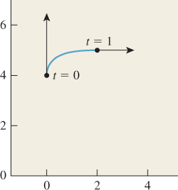
Figure 22.1: Animating a car’s motion. Given the initial and final points and velocity, we want to find a path like the magenta curve.
You need a way to “glue together” the two parts of the car’s path to get a smooth motion. What can you do? (We’re just looking for a smooth way to connect the “traveling along the y-axis” part of the path to the “traveling along the line y = 5” part, that is, the translational part of the car’s motion. We can then, at each instant, rotate the car to align it with the tangent to our interpolating path.
First, we generalize the problem: Given positions P and Q, and velocity vectors v and w, find a function γ :[0, 1] ![]() R2 such that γ(0) = P, γ(1) = Q, γ′ (0) = v, and γ′ (1) = w. The solution is given by
R2 such that γ(0) = P, γ(1) = Q, γ′ (0) = v, and γ′ (1) = w. The solution is given by

To check that γ(0) = P, we need only evaluate the four polynomials at t = 0; their values are 1, 0, 0, and 0.
Convince yourself that in fact the curve defined by γ satisfies γ(1) = Q, γ′ (0) = v, and γ′ (1) = w.
The resultant curve is called the Hermite (pronounced “airMEET”) curve for the data P, Q, v, and w. The four polynomials in Equation 22.1 are called the Hermite functions, or Hermite basis functions.
Everything in this example works equally well if P, Q, v, and w are in R3, or in R: It’s a dimension-independent construction. That’ll be true for all our subsequent curve types, too, and we won’t mention it again.
The four cubic polynomials in Equation 22.1 tell us how the inputs are combined to make the curve γ. In particular, the factors of t and (1 – t) in the polynomials for v and w tell us that these inputs have no influence on the locations of the endpoints γ(0) and γ(1), while the factor of t2 in the polynomial for Q shows that Q has no influence either on the location of γ(0) or on the tangent vector γ′ (0) (see Exercise 22.1 at the end of this chapter). The other polynomials can be read similarly. The graphs of these four polynomials, shown in Figure 22.2, reveal the same information.
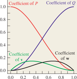
This is, as we said, an illustration of the Basis principle. In the Hermite basis, if we want to alter the starting point, we need only adjust the coefficient of the first polynomial; doing so will not alter the starting velocity, the ending point, or the ending velocity. If we had instead expressed the curve as a linear combination of the functions t ![]() t3, t
t3, t ![]() t2, t
t2, t ![]() t, and t
t, and t ![]() 1, then adjusting our solution in response to a change of starting point would have altered all the coefficients. The so-called “power basis” consisting of powers of t is the wrong choice for this problem; the Hermite basis is the right one.
1, then adjusting our solution in response to a change of starting point would have altered all the coefficients. The so-called “power basis” consisting of powers of t is the wrong choice for this problem; the Hermite basis is the right one.
We’ll generally use lowercase Greek letters (often γ) to name parametric curves, and we’ll generally use t as a parameter. Sometimes, however, we’ll need to relate two different curves, and in that case we will use s as well.
If the original problem had not been so nicely posed—if the original contact with the hill was at t = a, with velocity v, and the straight-line motion began at time t = b, with velocity w—we could still use an Hermite curve to solve it. We let c = b – a, and find the Hermite curve ζ for P, Q, c v, and cw. The gluing curve γ that we’re seeking is then given by
This kind of substitution works in great generality: If we find a function of t on [0, 1] with nice properties, we can transform it to a function of s on [a, b] with the substitution s = a + t(b – a), or ![]() .
.
The Hermite basis functions are all cubic polynomials. We can, by a small change in notation, write the polynomial a0 + a1t + a2t2 + a3t3 using matrix multiplication:
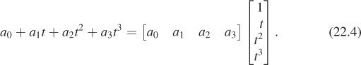
Letting t(t) denote a vector containing powers of t, or t(t) = [1 t t2 t3]T, we can write
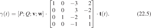
The first factor is a matrix, called the geometry matrix for the curve, and is denoted G. Its columns are the coordinates of P, Q, v, and w, respectively (we’ll use the semicolon notation for this in the future as well). The middle matrix, called the basis matrix and denoted M, contains the coefficients of the polynomials for the Hermite curve, from lowest to highest degree. ![]() In effect, it represents the change from the basis for cubic polynomials consisting of the four Hermite polynomials to the {1, t, t2, t3} basis.
In effect, it represents the change from the basis for cubic polynomials consisting of the four Hermite polynomials to the {1, t, t2, t3} basis.
(a) Multiply out, by hand, the second and third factors in the expression for γ(t); you should get a column vector of four polynomials. Confirm that these are the Hermite polynomials.
(b) Suppose that we had defined t to be the vector [t3 t2 t 1]T instead; how would the second matrix in the expression for γ(t) have to change to make the formula correct in this case?
Suppose that ζ(t) = (1 – t)P + tQ. Write ζ in a matrix form like that of Equation 22.5. Your vector t(t) will be just [1 t]T.
Thus, in brief, the Hermite curve can be written
All our subsequent curve formulations will have the form of Equation 22.6, namely, a geometry matrix G (which usually contains four points rather than two points and two vectors), a basis matrix M that lists the coefficients of some polynomials, and the vector T(t). The differences in various curve types are (a) the contents of the geometry matrix, and (b) the polynomials specified by the basis matrix.
22.3.1. Bézier Curves
Our second curve type is the Bézier curve. (Bézier is pronounced “BAY-zee-ay.”) It’s built from four points P1, ..., P4. The curve starts at P1, finishes at P4, and has initial velocity 3(P2 – P1) and final velocity 3(P4 – P3), as shown in Figure 22.3.
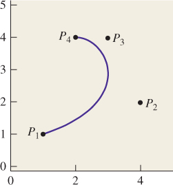
Figure 22.3: A Bézier curve starts at P1, heading toward P2, and ends at P4, coming from the direction of P3.
The Bézier curve is given by
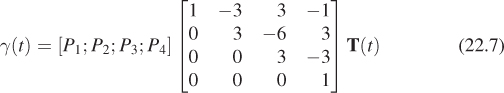
so that this time the geometry matrix contains the four points, and the basis matrix contains different coefficients.
It may seem that the Bézier specification is less natural than the Hermite form. The role of the points P2 and P3 is a little vague compared to that of the initial and final tangents. The advantage of the Bézier form is that all the specified items are points, so when we want to transform a Bézier curve we can simply transform the points. With an Hermite curve, we have to be careful about the distinction between transforming points and vectors, which you’ll recall from Chapter 12.
Suppose that P2 and P3 are evenly spaced between P1 and P4.
(a) Show that this means that G can be written
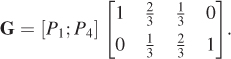
(b) Use the result of part (a) to show that in this case, γ(t) simplifies to just (1 – t)P1 + tP4, that is, a constant-speed, straight line from P1 to P4. This property is one reason why the factor of 3 is included in the definition of the Bézier curve.
Exercise 22.2 shows that there’s really very little difference between the two curve types.
22.4. Gluing Together Curves and the Catmull-Rom Spline
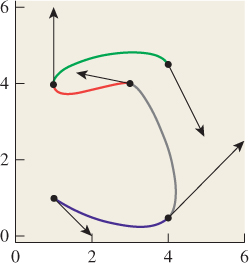
Suppose that we have a sequence of points P0, P2, ..., Pn and associated vectors v0, v2, ..., vn as shown in Figure 22.4, and we want to find a curve γ : [1, n] ![]() R2 that passes through these points with the given vectors as velocities. We can certainly use the Hermite formulation to find a curve γ0 : [0, 1]
R2 that passes through these points with the given vectors as velocities. We can certainly use the Hermite formulation to find a curve γ0 : [0, 1] ![]() R2 that starts at P0, ends at P1, and has initial and final tangents v0 and v1. We can also use it to find a curve γ1 :[0, 1]
R2 that starts at P0, ends at P1, and has initial and final tangents v0 and v1. We can also use it to find a curve γ1 :[0, 1] ![]() R2 that starts at P1, ends at P2, and has v1 and v2 as its initial and final tangents, and similarly can find curves γ3, ... γn–1. We can then define
R2 that starts at P1, ends at P2, and has v1 and v2 as its initial and final tangents, and similarly can find curves γ3, ... γn–1. We can then define
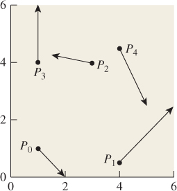
Figure 22.4: A sequence of points and vectors; we want a curve that passes through the points with the given vectors as velocities.
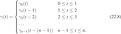
The resultant assembly of curves γ (Figure 22.5) is a continuous differentiable curve that passes through each point with the specified tangent. The individual pieces, t ![]() γi(t – i), are referred to as segments; the whole assembly is a spline, and the points and vectors are what we’ll call control data: They are the inputs that control the shape of the curve. In the most common case, we have just a sequence of points as our control data, and we call the points control points.
γi(t – i), are referred to as segments; the whole assembly is a spline, and the points and vectors are what we’ll call control data: They are the inputs that control the shape of the curve. In the most common case, we have just a sequence of points as our control data, and we call the points control points.
The Catmull-Rom spline is an example of a curve defined by a sequence of control points. It’s the solution to the problem, “Given a sequence of points P0, ..., Pn, find a smooth curve that passes through point i at time t = i, with the property that if the points are equispaced, the resultant curve is just a straight-line interpolation between the first and last points.”
The idea is simple: If we can just pick a tangent at each Pi, we can use Hermite curves as before. Thus, at each control point Pi, we need to pick a tangent. The Catmull-Rom idea is to use the previous and next control points as guides, that is, to pick the tangent vector at Pi to be in the direction Pi+1 –Pi–1 from the previous to the next control point. To satisfy the equispacing condition, we need to scale down this vector somewhat. We use the tangent vector vi = ![]() (Pi+1 – Pi–1), (i = 1, ..., n – 1).
(Pi+1 – Pi–1), (i = 1, ..., n – 1).
At the endpoint P0, this formula doesn’t work, because we don’t have a point P–1. So, for P0, we use ![]() , which is what we’d get with the general formula if there were a control point P–1 placed symmetric to P1 about P0, as shown in Figure 22.6.
, which is what we’d get with the general formula if there were a control point P–1 placed symmetric to P1 about P0, as shown in Figure 22.6.
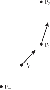
Figure 22.6: If we place a fictitious control point P–1 symmetric to P1 about P0, then we can define v0 = ![]() (P1 – P–1). Notice that the tangent at P1 is parallel to the line from P0 to P2.
(P1 – P–1). Notice that the tangent at P1 is parallel to the line from P0 to P2.
Similarly, for Pn we use ![]() . The result, after a lot of algebraic shuffling that’s described in the web material for this chapter, can be written in the form
. The result, after a lot of algebraic shuffling that’s described in the web material for this chapter, can be written in the form
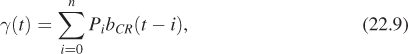
where bCR is the Catmull-Rom curve shown in Figure 22.7 and defined by
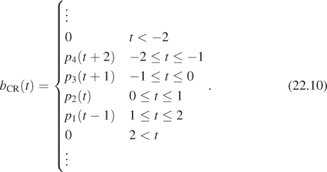
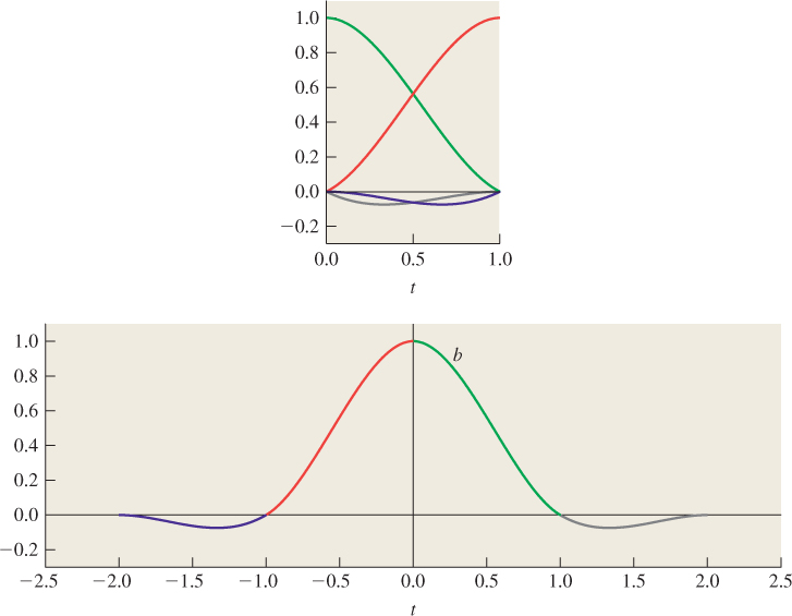
Figure 22.7: The four Catmull-Rom basis functions, plotted on a single coordinate system, and then shifted and assembled to form the function bCR defined on the interval [−2, 2]. Because bCR is continuous and is C1 smooth, so is the Catmull-Rom spline. Because bCR(0) = 1, while bCR(i) = 0 for all other integers i, the Catmull-Rom spline is interpolating.
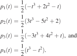
where
The form of the Catmull-Rom curve given in Equation 22.9 is convenient for studying the properties of Catmull-Rom splines. Note that, although the sum appears to have n terms, for any particular value of t there are, at most, four nonzero terms. This means that it’s easy to write code to rapidly determine points on a Catmull-Rom spline. The function bCR goes below 0 at some times. This means that the sum in Equation 22.9 is not a convex combination of the control points: The interpolating curve for control points Po, ..., Pn may go outside the convex hull of these points. Figure 22.8 shows a simple example. It’s a sad fact that if you want a smooth interpolating curve (i.e., one that passes through the control points rather than near them), this failure to stay within the convex hull is unavoidable.
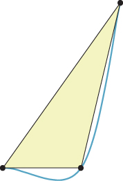
Figure 22.8: The Catmull-Rom spline for three control points lies almost entirely outside the yellow triangular convex hull of the three points.
Note that the function bCR is infinitely differentiable at most points (because it’s polynomial), but at the joint points (x = –2, –1, 0, 1, 2) it’s only once differentiable. This is fine in some simple modeling applications, but you would not want to use a Catmull-Rom spline curve as a path for a dollied camera, for example: The resultant camera motion would seem very jerky to the viewer.
22.4.1. Generalization of Catmull-Rom Splines
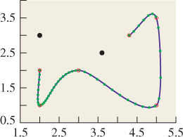
We can generalize and say, “Given P0, ..., Pn and a sequence of parameter values t0 < ... < tn, find a curve γ such that γ(ti) = Pi for i = 0, ... n.” These parameter values ti are called knots, and the sequence of knots is denoted by the letter T = t0, t1, ..., tn. Figure 22.9 shows a spline with knots at t = 0, 1, 3, 4.3, 3.8, 5.5 and control points drawn as red circles; the large blue dots are the fictitious control points. The 50 green dots are equispaced from 1 to 5.5 to show the velocity of the curve.
The basic Catmull-Rom spline has its knots at t = 0, 1, 2, ...; the constant inter-knot spacing leads to the name uniform for this kind of spline. In this section, we’re describing the generalization to a nonuniform Catmull-Rom spline.
To solve the general problem of finding the nonuniform Catmull-Rom spline for a given sequence of knots and control points, we once again add a fictitious pre-start point P–1 = P0 – (P1 – P0), but we also add a pre-start knot, t–1 = t0 – (t1 – t0), and corresponding post-end point and knot. The ith segment of the curve is controlled by points Pi–1, Pi, Pi+1, Pi+2 and is defined for t ![]() [ti, ti+1], but it is influenced by ti–1 and ti+2 as well. The four blending functions for this ith segment, t
[ti, ti+1], but it is influenced by ti–1 and ti+2 as well. The four blending functions for this ith segment, t ![]() pi,1(T, t), t
pi,1(T, t), t ![]() pi,2(T, t), t
pi,2(T, t), t ![]() pi,3(T, t), and t
pi,3(T, t), and t ![]() pi,4(T, t), which are used to blend Pi–1, Pi, Pi+1, and Pi+2, are given by
pi,4(T, t), which are used to blend Pi–1, Pi, Pi+1, and Pi+2, are given by
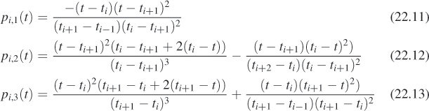
and
For the special case ti = i, these agree with the Catmull-Rom basis functions given in the previous section.
To make this concrete, suppose we specify a nonuniform Catmull-Rom spline in the plane with the data
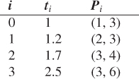
and we wish to evaluate the spline curve at many t-values so as to make a polyline that closely approximates it.
First, we add the two fictitious control points to the table:
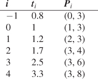
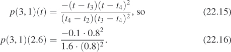
Now, to evaluate the curve at a particular t-value like t = 2.6, for example, we determine that t3 ≤ 2.6 ≤ t4. This means that we’re in the ith segment, where i = 3. We’ll therefore need to evaluate p(3, 1)(t), ..., p(3, 4)(t).
In evaluating the other three polynomials, the expressions t – ti and ti+1 – t appear repeatedly. To write efficient code, you’d want to evaluate these just once and reuse them often.
22.4.2. Applications of Catmull-Rom Splines
Suppose that you’re doing an animation in which you have a moving object, and you want it at position Pi at time ti for i = . . .; the Catmull-Rom spline is a natural choice. Now suppose you’ve got an object that’s controlled by some parameter such as a pinwheel whose rotation is specified in degrees at several key times—say, R(0) = 45, R(1) = 360, and R(3) = 720—and you want to provide values for R at intermediate times. Again, the Catmull-Rom spline is a natural choice. Note, however, that if the rotations were specified by R(0) = R(1) = 0 and R(3) = 90, then the Catmull-Rom interpolant, at t = 0.5, would be negative: The pinwheel would start to spin backward before rushing to spin forward. While this might give the feeling of anticipation of motion in a cartoon-like animation, it would be inappropriate for an animation that was supposed to be physically realistic.
22.5. Cubic B-splines
Cubic B-splines (there are also linear, quadratic, quartic, etc., B-splines, but cubics are widely used) are similar to Catmull-Rom splines. The key differences are that the cubic B-spline (a) is C2 smooth, that is, both its first and second derivatives are continuous functions, and (b) is noninterpolating, that is, it passes near the control points, but not through them in general.
Cubic B-splines come in two flavors: uniform and nonuniform. We’ll start with the uniform B-spline. The formula for the cubic B-spline with control points P0, ..., Pn is
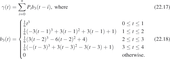
The domain of the curve γ is 0 ≤ t ≤ n – 2. Because of the structure of the function b3, it turns out that for j ≤ t ≤ j + 1, the point γ(t) lies in the convex hull of the four points Pj–3, ..., Pj. This convex hull property is useful in computing the intersection of a ray with a B-spline: If the ray misses the convex hull of four sequential control points, it also must miss the corresponding segment of the B-spline curve. If the ray hits the convex hull, then further computation is needed. The web material for this chapter gives details.
Just like the Bézier and Hermite curves, a segment of a B-spline can be expressed in a matrix form, which can make evaluation more efficient. Recall that the form for the Bézier and Hermite curves was
where T(t) is the vector [1 t t2 t3]T of powers of t. Because a B-spline curve is made of many segments, defined for 0 ≤ t ≤ 1, 1 ≤ t ≤ 2, etc., we’ll end up using T(t – j) for the jth segment, that is, a vector of powers of the fractional part of t.
For the jth segment, defined for j ≤ t ≤ j+1, and influenced by control points Pj–3, ..., Pj, we define a geometry matrix
which is 2 × 4 for curves in the plane, or 3 × 4 for curves in space, and contains the coordinates of the control points as columns of the matrix. We multiply this by the B-spline basis matrix, MBs:
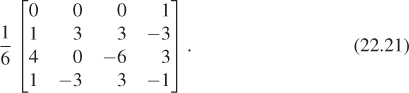
The uniform B-spline curve is then
where j = ![]() t
t![]() so that t – j is the fractional part of t.
so that t – j is the fractional part of t.
Although B-splines don’t pass through their control points, their extra degree of continuity makes them attractive in many applications. The tradeoff between controllability (does the curve interpolate its control points?) and continuity (how smooth is it?) is one that must be managed on a case-by-case basis in applications.
22.5.1. Other B-splines
While B-splines (and other cubic or piecewise-cubic curve formulations) are very popular, they do have limitations. One is that with a finite set of control points, you cannot make a B-spline curve traverse a unit circle. Since circles are important in manufacturing and many other applications, this is a severe limitation.
The solution is to include an extra coordinate, w, in your B-spline. You then take (x(t), y(t), w(t)) and treat it as defining ![]() ; the resultant curve is called a rational B-spline, and it happens that with a rational B-spline, you can traverse a circle and other conic sections.
; the resultant curve is called a rational B-spline, and it happens that with a rational B-spline, you can traverse a circle and other conic sections.
The uniform spacing of B-splines is a convenience . . . unless you have data that happens to have nonuniform spacing (e.g., you know the position of an object in an animation at times t = 0, 1, 2, and 10). For this situation, there’s a generalization of the B-spline called the nonuniform B-spline, and the rational version of this—the nonuniform rational B-spline or NURB—is one of the tools of choice in many CAD systems. One advantage of nonuniform B-splines is that by repeating knots (i.e., by having both t3 and t4 have the same value), you can reduce the continuity of the curve at t3, allowing a user to put sharp corners into an otherwise smooth piecewise cubic curve, for instance. The web materials describe the uses of repeated control points and repeated knots in shaping NURBS curves.
22.6. Subdivision Curves
As you saw in Chapter 4, repeated subdivision of a polygonal curve can lead to a smooth curve. There’s one particular subdivision rule with some great properties. The new polygon is derived from the old one by doing the following:
• Using the midpoint of the edge from vi to vi+1 as the vertex we’ll call ei (for “edge”)
• Replacing ![]() (which is only defined for 0 < i < n)
(which is only defined for 0 < i < n)
• Creating the new polygon e1, w1, e2, w2, ..., en–1
Figure 22.10 shows an example of several levels of subdivision, where the rule has been extended to i = 0 and i = n using indices modulo n. The limit curve (with this subdivision scheme) turns out to be smooth. Figure 22.11 shows an advantage of subdivision as a modeling approach: You can draw the general shape of a curve with a first polygon, subdivide a couple of times, and then move a single control point to introduce a finer-scale feature, and continue subdividing.
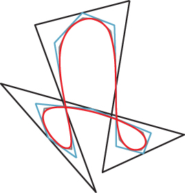
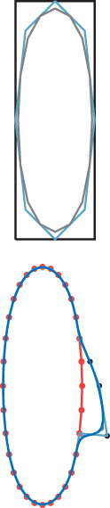
Figure 22.11: The large-scale shape of a face is drawn at the top as a black rectangle; after two levels of subdivision (shown as a red oval at the bottom), three control points (in black) are moved to the right to make a nose, and further subdivision generates a smooth curve (blue).
Even though subdivision is easy to perform, it’s nice to know a parametric form for the limit curve. Figure 22.12 shows that if we take the polyline with vertices ..., (–2, 0), (–1, 0), (0, 1), (1, 0), (2, 0), ... and subdivide it, the successive curves rapidly approach the B-spline curve b3 of Equation 22.18, which we’ve drawn as a solid red curve at the bottom. With a good deal of linear algebra, you can show that this apparent limit is in fact exact: Subdivision is just another way of describing cubic B-spline curves.
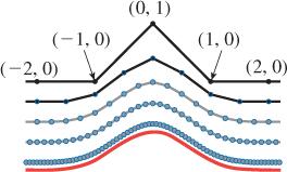
Figure 22.12: The control polygon at the top, when subdivided, approaches the graph of b3 (in red), the cubic B-spline function. The subdivision levels are drawn vertically offset for clarity.
What makes subdivision important (aside from its simplicity) is that it generalizes very nicely to surfaces, which we’ll discuss in the next chapter.
22.7. Discussion and Further Reading
The web material for this chapter includes a much-expanded version of the material you’ve just read, and includes topics such as spline paths that are “circular” (i.e., that start and end at the same point, with the same tangent vector, so you can use them for describing repeated motions). It also contains pointers to other literature on the subject.
One of the early reasons for developing splines was to approximate other functions with comparatively simple ones. This idea leads naturally to the use of splines for compression: If you have a sequence of many data points that lie on a fairly smooth curve, you can probably approximate that curve with a spline curve defined by just a few control points, thus generating a lossy compression of the data. This is really just a generalization of the idea of approximating data by fitting lines to them, but it’s quite powerful.
22.8. Exercises
Exercise 22.1: The four Hermite polynomials of Equation 22.1 control the shape of the Hermite curve.
(a) Compute the derivative of each polynomial.
(b) Evaluate the derivatives at t = 0 and t = 1.
(c) Explain why only v and w affect the direction of the Hermite curve at the start and end, while P and Q have no effect on these directions.
Exercise 22.2: An Hermite curve specification has a geometry matrix GH = [P, Q, v, w] containing the two endpoints and their associated tangents. A Bézier curve specification contains four points GB = [P1 P2 P3 P4]. They each, too, have associated basis matrices, which we’ll call MH and MB, respectively. (a) Show that if we pick
then the Hermite curve defined by P, Q, v, and w is identical to the Bézier curve defined by P1, ..., P4.
(b) Show that in this situation, in matrix form, we have
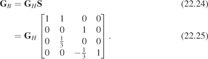
(c) Using the fact that GBMB = GHMH, and part (b), show how to determine MH from MB.![]() (The equality of the two products holds because if At(t) = Ct(t) for every t for two 4 × 4 matrices A and C, then A = C; that’s because the vectors t(0), t(1), t(2), and t(3) are linearly independent.)
(The equality of the two products holds because if At(t) = Ct(t) for every t for two 4 × 4 matrices A and C, then A = C; that’s because the vectors t(0), t(1), t(2), and t(3) are linearly independent.)
Exercise 22.3: In the development of the Catmull-Rom spline, we talked about placing a fictitious control point P–1 that’s symmetric to P1 about P0.
(a) Show that the point P–1 is given by P0 – (P1 – P0), and simplify.
(b) Show that if we apply the rule ![]() , then the formula from part (a) lets us simplify this to
, then the formula from part (a) lets us simplify this to ![]() .
.
Exercise 22.4: In the Catmull-Rom spline, we placed a fictitious control point at each end, placing it so that the last three control points at each end were symmetrical. What would happen if we set P–1 = P0 and Pn+1 = Pn instead? The resultant spline will still interpolate all the original control points, but thinking of the spline as describing the position of a moving point at time t, we’ll see its motion change at the ends. How will it change?
Exercise 22.5: Show that the Catmull-Rom spline is in general not C2. On each segment, the second derivative is a linear function (as it is for any cubic spline). Show that this function need not be continuous between segments.