
Chapter 32. Rendering in Practice
32.1. Introduction
In this chapter we show implementations of two renderers—a path tracer and a photon mapper—with some of the optimizations that make them worth using. Both approaches are currently in wide use, are fairly easy to understand, and form complete solutions to the rendering problem in the sense that they can be shown (under reasonable conditions) to provide consistent estimates of the values we seek (i.e., “properly” rendered images).
We’re not recommending these as ideal renderers. Rather, we treat them as case studies. They are rich enough to exhibit of the complexities and features of a modern renderer; they provide the foundation necessary for you to read research papers on rendering.
We assume that you’ve implemented the basic ray tracer described in Chapter 15. Much of this chapter also depends heavily on Chapters 30 and 31.
In the course of implementing these renderers, we describe ways to structure the representation of geometry in a scene, of scattering, and of samples that contribute to a pixel. These are not always in a form immediately recognizable from the mathematical formulation of the previous chapters, as you’ll know from Chapter 14.
In Section 32.8, we discuss the debugging of rendering programs, showing some example failures and their causes, and suggesting how you can learn to identify the kind of bug from the kind of visual artifacts you see.
32.2. Representations
As you build a ray-casting-based renderer, your choices of representations will have large-scale impacts. Is the scattering model you’ve chosen rich enough to represent the phenomena you wish to simulate? Is it easy to sample from a probability distribution proportional to ω ![]() fs(ωi,ω)|ω · n| for some fixed vector ωi? Is your scattering energy-conservative? Does your scene representation make ray-scene intersection fast and robust? Does your representation of luminaires make it easy to select points on a luminaire uniformly with respect to area?
fs(ωi,ω)|ω · n| for some fixed vector ωi? Is your scattering energy-conservative? Does your scene representation make ray-scene intersection fast and robust? Does your representation of luminaires make it easy to select points on a luminaire uniformly with respect to area?
For each of the questions above, describe how a basic ray tracer’s output or running time might be affected by the answer being “Yes” or “No.”
Beyond these choices, there are the practical matters of modeling. For instance, the scattering properties of a surface are usually defined or measured relative to the surface normal (and perhaps relative to a tangent basis as well), while we’ve treated the scattering model (or at least the bidirectional scattering distribution function or BSDF) as a function of a point in space and two direction vectors. In practice, of course, we trace a ray to find a point of some surface, and then find the BSDF at that point as a surface property, with its parameters being determined both by surface position and by various texture maps. We’ll begin by discussing this particular simplification.
32.3. Surface Representations and Representing BSDFs Locally
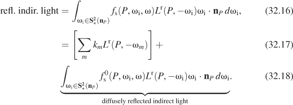
Consider a patch of surface so small that it may locally be considered flat, and a local coordinate frame at a point P, with unit normal vector n and unit tangent vectors u and v such that u, v, n is an orthonormal basis of 3-space, as shown in Figure 32.1. This decomposition of a surface into a tangent space and a normal space depends on local flatness; it’s problematic at edges and corners (like those of a cube), where it’s not obvious which directions should be called “tangent” or “normal.” This is a real problem for which graphics has yet to determine a definitive answer.
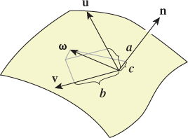
Figure 32.1: A local basis at a point P, consisting of mutually perpendicular unit vectors. The vector ω is shown being decomposed into a linear combination of these via dot products.
For any vector ω at P, we can easily represent ω = au + bv + cn, by computing dot products: a = ω · u, etc.
If ω, n, u, and v are expressed in world coordinates, and M is a 3 × 3 matrix whose rows are u, v, and n, then show that  Knowing this lets us convert from world coordinates to local tangent-plus-normal coordinates.
Consider now the BSDF fs(P, ωi, ωo), which is a function of a surface point and two (unit) vectors at that point. If we write ωi = au + bv + cn and ωo = a′u + b′v + c′n, we can define a new function,
We can go further, however. Since ωi and ωo are unit vectors, we can express them in polar coordinates using φ for longitude and θ for latitude, corresponding to the standard use of θ for the angle between ω and n. This gives θ = cos–1(b) and φ = atan2(c, a), and we can write
The function ![]() r is what a gonioreflectometer actually measures. Notice that fs and
r is what a gonioreflectometer actually measures. Notice that fs and ![]() r are merely different representations of the same thing, like the rectangular- or polar-coordinate representations of a curve. (We discussed such shifts of representation in Chapter 14)
r are merely different representations of the same thing, like the rectangular- or polar-coordinate representations of a curve. (We discussed such shifts of representation in Chapter 14)
The function ![]() s has a form in which certain common properties of BSDFs can be easily expressed. For instance, the Lambertian bidirectional reflectance distribution function (BRDF) is completely independent of θo, φi, and φo. Because of this, the particular choice of u and v is irrelevant for the Lambertian BRDF: The dot products of ωi and ωo with u and v are only used in computing φi and φo.
s has a form in which certain common properties of BSDFs can be easily expressed. For instance, the Lambertian bidirectional reflectance distribution function (BRDF) is completely independent of θo, φi, and φo. Because of this, the particular choice of u and v is irrelevant for the Lambertian BRDF: The dot products of ωi and ωo with u and v are only used in computing φi and φo.
The Phong and Blinn-Phong BRDFs both depend on θi and θo, but their dependence on φi and φo is rather special: They depend only on the difference of φi – φo (indeed, on this difference taken mod 2π).
(a) Explain the claim that the Blinn-Phong BRDF depends only on the difference of φi and φo.
(b) Show that in fact it depends only on the magnitude of the difference: The sign is irrelevant.
This dependence on the difference in angles again means that the BSDF expressed in (θ, φ) terms, ![]() s, is independent of the choice of u and v: If we rotated these in the tangent plane by some amount α, then both φi and φo would change by α (and possibly by an additional 2π), and their difference (mod 2π) would remain invariant. BSDFs with this property are said to be isotropic, and they can be represented by functions of the three variables θi, θo, and φ = (φi – φo) mod 2π. The great majority of materials currently used in graphics are represented by BSDFs (indeed, BRDFs) that fall into this category; the exceptions (anisotropic materials) are things like brushed aluminum, in which the brushing direction introduces an anisotropy. Materials that are represented using subsurface scattering often have interior structure that makes them anisotropic as well, so the simplified representation is often inapplicable to those.
s, is independent of the choice of u and v: If we rotated these in the tangent plane by some amount α, then both φi and φo would change by α (and possibly by an additional 2π), and their difference (mod 2π) would remain invariant. BSDFs with this property are said to be isotropic, and they can be represented by functions of the three variables θi, θo, and φ = (φi – φo) mod 2π. The great majority of materials currently used in graphics are represented by BSDFs (indeed, BRDFs) that fall into this category; the exceptions (anisotropic materials) are things like brushed aluminum, in which the brushing direction introduces an anisotropy. Materials that are represented using subsurface scattering often have interior structure that makes them anisotropic as well, so the simplified representation is often inapplicable to those.
The preceding discussion has been in terms of the angles θi, φi, θo, and φo to emphasize that the BSDF is a function on a four-dimensional domain. In practice, however, it is the sines and cosines of these angles that most often enter into the computations, at least for analytically expressed BSDFs. (For tabulated BSDFs, we can tabulate based not on θi and θo, but on their cosines, so the same argument applies to those.) In practice, a BSDF implementation will typically take a point, P, and the two vectors ωi and ωo, and promptly express these vectors in terms of u, v, and n.
How does all this look in an implementation? Part of G3D’s implementation of a generalized Blinn-Phong model is shown in Listing 32.1.
There are several design choices here. The first is that a SurfaceElement is used to represent the intersection of a ray with a surface in the scene. Among other things, it has data members material and shading. The material stores things like the Phong exponent, the reflectivities in the red, green, and blue spectral regions, etc. The shading stores the intersection point, the texture coordinates there, and the surface normal there. (It may help, when reading expressions like p.shading.normal, to treat “shading” as an adjective. Thus, p.shading.normal is the shading normal, while p.geometric.normal is the geometric normal.)
Listing 32.1: Part of an implementation of Blinn-Phong reflectance.
1 Color3 SurfaceElement::evaluateBSDFfinite(w_i, w_o) {
2 n = shading.normal;
3 cos_i = abs(w_i.dot(n));
4
5 Color3 S(Color3::zero());
6 Color3 F(Color3::zero());
7 if ((material.glossyExponent != 0) && (material.glossyReflect.nonZero())) {
8 // Glossy
9
10 // Half-vector
11 const Vector3& w_h = (w_i + w_o).direction();
12 const float cos_h = max(0.0f, w_h.dot(n));
13
14 // Schlick Fresnel approximation:
15 F = computeF(material.glossyReflect, cos_i);
16 if (material.glossyExponent == finf())
17 S = Color3::zero()
18 } else {
19 S = F * (powf(cos_h, material.glossyExponent) * ...
20 }
21 }
22 ...
The surface normal is used immediately to compute cos θi, an example of expressing one of the two input vectors in the local frame of reference. The half-vector (direction() returns a unit vector) is computed from ωi and ωo, which are called w_i and w_o in the code. The Schlick approximation of the Fresnel term is computed and used to determine the glossy reflection. The remainder of the elided code computes the diffuse reflection. Missing from this code are the evaluations of the mirror-reflection term and of transmittance based on Snell’s law, each of which corresponds to an impulse in the scattering model. The splitting off of these impulse terms makes the computation of the reflected light much simpler. Recall that what we’ve been expressing as an integral, namely,
is really shorthand for a linear operator being applied to L, one that is defined in part by a convolution integrand like the one above, and in part by impulse terms like mirror reflectance, where for a particular value of ωi, the integrand is nonzero only for a specific direction ωo; the value of the “integral” is some constant (the impulse coefficient) times L(P, –ωi).
Trying to approximate terms like mirror reflectance by Monte Carlo integration is hopeless: We’ll never pick the ideal outgoing direction at random. Fortunately, these terms are easy to evaluate directly, so no approximation is needed. The SurfaceElement class therefore provides a method (see Listing 32.2) that returns all the impulses needed to evaluate the reflected radiance (in this case, the mirror-reflection impulse and the transmission impulse, although if we were rendering a birefringent material, there would be two transmissive impulses, so returning an array of impulses is natural).
G3D is designed around triangle meshes. The SurfaceElement class therefore contains some mesh-related items as well (see Listing 32.3).
Listing 32.2: A method that returns the impulse parts of a scattering model.
1 void getBSDFImpulses (Vector3& w_i, Array<Impulse>& impulseArray) {
2 const Vector3& n = shading.normal;
3
4 Color3 F(0,0,0);
5
6 if (material.glossyReflect.nonZero()) {
7 // Cosine of the angle of incidence, for computing
8 //Fresnel term
9 const float cos_i = max(0.001f, w_i.dot(n));
10 F = computeF(material.glossyReflect, cos_i);
11
12 if (material.glossyExponent == inf()) {
13 // Mirror
14 Impulse& imp = impulseArray.next();
15 imp.w = w_i.reflectAbout(n);
16 imp.magnitude = F;
17 ...
Listing 32.3: Further members of the SurfaceElement class.
1 class SurfaceElement {
2 public:
3 ...
4 struct Interpolated {
5 /** The interpolated vertex normal. */
6 Vector3 normal;
7 Vector3 tangent;
8 Vector3 tangent2;
9 Point2 texCoord;
10 } interpolated;
11
12 /** Information about the true surface geometry. */
13 struct Geometric {
14 /** For a triangle, this is the face normal. This is useful
15 for ray bumping */
16 Vector3 normal;
17
18 /** Actual location on the surface (it may be changed by
19 displacement or bump mapping later. */
20 Vector3 location;
21 } geometric;
22 ...
The vectors tangent and tangent2 correspond to u and v above; when the surface is modeled, these must be specified at every vertex. Using the derivative of texture coordinates is one way to generate these; if we have texture coordinates (ui, vi) at vertex i, we can find a linear approximation for u across the interior of the triangle, and from this determine a direction u in which u grows fastest. We can then define v as n×u to get an orthonormal basis. Note, however, that this is a per-triangle computation, and the computation of u is not guaranteed to be consistent across triangles. Indeed, because of the mapmaker’s dilemma (you can’t flatten the globe onto a single piece of paper preserving angles and distances), the consistent assignment of texture coordinates across a whole surface is generally impossible. It’s important that any anisotropic BRDF be used only in areas where u and v are defined consistently.
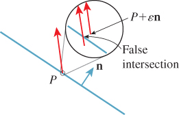
The vector geometric.normal is the triangle-face normal rather than the surface normal that it approximates. Depending on how the surface was originally modeled, these may be identical, or the surface normal may be some weighted combination of face normals, or it may be determined by some other method entirely. The triangle-face normal is useful in ray-tracing algorithms because if P is a point that’s supposed to lie on a triangle T (see Figure 32.2), it may be that a ray traced from P into the scene first hits the scene at a point of T, because a roundoff or representation error places P slightly to one side of T. By slightly displacing (bumping) P along the normal to T, that is, by replacing P with P+![]() n for some small
n for some small ![]() , we can avoid such false intersections. (Perhaps “nudging” would be a better term, to avoid conflict with the notion of bump-mapping, but “bumping” is the term used by G3D.) How large should
, we can avoid such false intersections. (Perhaps “nudging” would be a better term, to avoid conflict with the notion of bump-mapping, but “bumping” is the term used by G3D.) How large should ![]() be? A good rule of thumb is “no more than 1% of the size of the smallest object you expect to see in the scene.” This implicitly establishes a condition on your models: No significant object or feature should be less than 100 times the largest gap between two adjacent floating-point numbers of the size you will be using. For instance, if everything in your scene will have coordinates between −100 and 100, and you will use IEEE 32-bit floating-point numbers, then since the largest gap between two floating-point numbers near 100 is about 4 × 10⁻⁶, you should not expect to model any feature smaller than 4 × 10⁻⁴ units.
be? A good rule of thumb is “no more than 1% of the size of the smallest object you expect to see in the scene.” This implicitly establishes a condition on your models: No significant object or feature should be less than 100 times the largest gap between two adjacent floating-point numbers of the size you will be using. For instance, if everything in your scene will have coordinates between −100 and 100, and you will use IEEE 32-bit floating-point numbers, then since the largest gap between two floating-point numbers near 100 is about 4 × 10⁻⁶, you should not expect to model any feature smaller than 4 × 10⁻⁴ units.
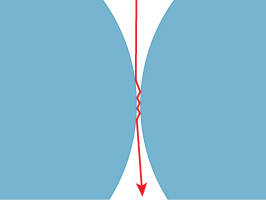
If we’re tracing a ray P + td, we could “bump” P along the ray, that is, bump it slightly in the direction d. Argue that this is a bad idea by considering rays that are almost tangent to the surface.
32.3.1. Mirrors and Point Lights
If we allow point lights in the scene, then when we trace rays “from the eye,” we’ll hit the point light with probability zero, so that it’ll almost never happen in practice. Similarly, if we allow perfect mirrors, we cannot write the scattering operator as an integral to be approximated by naive sampling—we’ll essentially never sample the direction of the mirror-reflected ray. When we combine the two, things are even worse.
Consider a scene consisting of a smooth mirrored ball illuminated by a point light. If we ray-trace from the eye through the pixel centers, we’ll almost certainly miss the point light; if we ray-trace from the light, we’ll miss the pixel centers. But if we suppose that the point light is in the scene as a proxy for a spherical light of some small radius r, then we know that we should see a highlight on the mirrored ball.
Losing that highlight is perceptually significant, even though the highlight might appear at only a single pixel of the image. We have three choices: We can abandon the convenient fiction of a point light, we can adjust the BRDF to compensate for the abstraction, or we can choose some other method for estimating the radiance arriving at the eye from that location. In an ideal world, with infinite rendering resources, we’d choose to use tiny point lights and cast a great many rays. Within the context of ray tracing, we can clamp the maximum shininess (i.e., the specular exponent) when we are combining a BRDF with a direct luminaire in the reflection operator. This ensures that with sufficiently fine sampling, the point light will produce a highlight. Of course, it also slightly blurs the reflection of every other object in the scene. The difference in appearance between a specular exponent of 10,000 and ∞ tends to be unnoticeable in general, so this is an acceptable compromise. On the other hand, if the specular exponent is 10,000, a very fine sampling around the highlight direction is required, or else we’ll get high variance in our image. This leads us to the third alternative. It may make sense to separate out the impulse reflection of point lights (or even small lights) into a separate computation to avoid these sampling demands, but we will not pursue this approach here.
32.4. Representation of Light
In our theoretical discussion, we treated light as being defined by the radiance field (P, ω) ![]() L(P, ω): At any point P, in any direction ω, L(P, ω) represented the radiance along the ray through P in direction ω, measured with respect to a surface at P perpendicular to ω. When P is in empty space, this is a good abstraction. When P is a point exactly on a surface, there are two problems.
L(P, ω): At any point P, in any direction ω, L(P, ω) represented the radiance along the ray through P in direction ω, measured with respect to a surface at P perpendicular to ω. When P is in empty space, this is a good abstraction. When P is a point exactly on a surface, there are two problems.
1. The precise relationship between geometric modeling and physics has been left undefined. We haven’t said whether a solid is open (i.e., does not contain its boundary points, like an open interval) or closed; equivalently, we haven’t said whether a ray leaving from a surface point of a closed surface intersects that surface or not.
2. When P is a point on the surface of a transparent solid, like a glass sphere, and ω points into the solid (see Figure 32.4), there are two possible meanings for L(P, ω): the light arriving at P from distant sources, or the light traveling from P into the interior of the surface. Because of Snell’s law, material opacity, and internal reflection, these two are almost never the same.
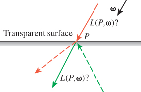
We addressed the second problem in Chapter 26, by defining an incoming and outgoing radiance for each pair (P, ω), where P was a surface point and ω was a unit vector, by comparing ω with the normal n(P) to the surfaces; we also mentioned that Arvo’s division of the radiance field into field radiance and surface radiance accomplishes the same thing.
For the first problem, we will say that a point on the boundary of a solid is actually part of that solid, so a point P on the surface of a glass ball is actually part of the ball (and for a varnished piece of wood, a point on the boundary is treated as being in both the varnish and the wood). This means that a ray leaving P in the direction nP first intersects the ball at P. (As a practical matter, avoiding the intersection at t = 0 requires a comparison of a real number against zero, which is prone to floating-point errors, so including the first hit point is easier than avoiding it.) Thus, with this model of surface points, the notion of “bumping” is not merely a convenience for avoiding roundoff error problems, it’s a necessity.
32.4.1. Representation of Luminaires
32.4.1.1. Area Lights
Our simple scene model supports a very basic kind of area light: We represent area light sources with a polygon mesh (often a single polygon) and an emitted power Φ. At each point P of a polygon, light is emitted in every direction ω with ω · nP > 0; the radiance along all such rays, in all directions, is constant over the entire luminaire.
The radiance along each ray can be computed by dividing the luminaire’s power among the individual polygons by area; we thus reduce the problem to computing the radiance due to a single polygon of area A and power Φ. That radiance is ![]() , as we saw in Section 26.7.3.
, as we saw in Section 26.7.3.
We will need to sample points uniformly at random (with respect to area) on a single area light. To do so, we compute the areas of all triangles, and form the cumulative sums A1, A1 + A2, ..., A1 + ... + Ak = A, where k is the number of triangles. To sample at random, we pick a uniform random value u between 0 and A; we find the triangle i such that A1 + ... + Ai ≤ u, and then generate a point uniformly at random on that triangle (see Exercise 32.6).
We’ll also want to ask, for a given point P of the surface and direction ω with ω · nP > 0, what is the radiance L(P, ω)? For our uniformly radiating luminaires, this is a constant function, but for more general sources, it may vary with position or direction.
32.4.1.2. Point Lights
Point-light sources are specified by a location1 P and a power Φ. Light radiates uniformly from a point source in all directions. As we saw in Chapter 31, it doesn’t make sense to talk about the radiance from a point source, but it does make sense to compute the reflected radiance from a point source that’s reflected from a point Q of a diffuse surface. The result is
1. We only allow finite locations; extending the renderer to correctly handle directional lights is left as a difficult exercise.
If a point light hits a mirror surface or transmits through a translucent surface, we can then compute the result of its scattering from the next diffuse surface, etc. This eventually becomes a serious bookkeeping problem, and since point lights are merely a convenient fiction, we ignore it: We compute only diffuse scattering of point lights. Although addressing this properly in a ray-tracing-based renderer is difficult, we’ll see later that in the case of photon mapping, it’s quite simple.
One useful compromise for point-light sources is to say that for the purpose of emission directly toward the eye, the point source is actually a glowing sphere of some small radius, r, while when it’s used in the calculation of direct illumination, it’s treated as a point. This compromise, however, has the drawback that it requires the design of the class for representing lights to know something about the kinds of rays that will be interacting with it (i.e., an eye ray will be intersection-tested against a small sphere, while a secondary ray will never meet the light source at all), which violates encapsulation.
32.5. A Basic Path Tracer
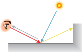
Recall the basic idea of ray tracing and path tracing: For each pixel of the image, we shoot several rays from the eye through the pixel area. A typical ray (the red one in Figure 32.5) hits the scene somewhere, and we compute the direct light arriving there (the nearly vertical blue ray), and how it scatters back along the ray toward the eye (gray). We then trace one or more recursive rays (such as the yellow ray that hits the wall), and compute the radiance flowing back along them, and how it scatters back toward the eye, etc. Having computed the radiance back toward the eye along each of the rays through our pixel, we take some sort of weighted average and call that the pixel value.
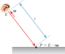
Because of the usual description of ray tracing (“Start from the eye, and follow a ray out into the scene until it hits a surface at some point P, and ...”), we’ll use the convention that the rays we discuss are always the result of tracing from the eye, that is, the first ray points away from the eye, the second ray points away from the first intersection toward a light or another intersection, etc. (see Figure 32.6).

Figure 32.6: The algorithm works from the eye toward the light source (red); photons travel in the opposite direction (blue).
On the other hand, the radiance we want to compute is the radiance that flows along the ray in the other direction. If the eye ray r starts at the eye, E, and goes in direction ω, meeting the scene at a point P, then we want to compute L(P, –ω), that is, we want to compute the radiance in the opposite of r’s direction. We’ll have various procedures like Radiance3 estimateTotalRadiance(Ray r, ...); such functions always return the radiance flowing in the direction opposite that of r.
32.5.1. Preliminaries
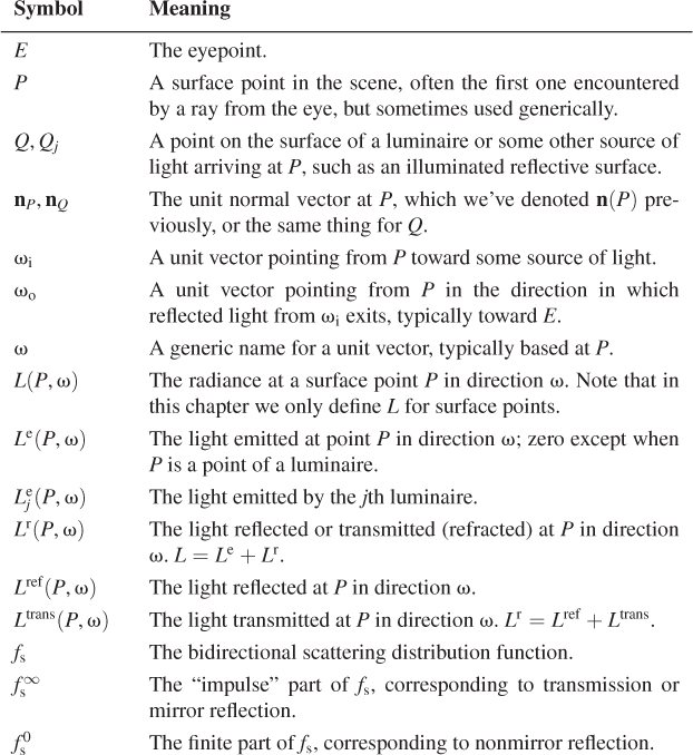
We begin with a very simple path tracer, in which the image plane is divided into rectangular areas, each of which corresponds to a pixel. If a ray toward the eye passes through the (i, j)th rectangle, we treat the radiance as a sample of the radiance arriving at that rectangle. Despite the simplicity of the path tracer, we’ll use a lot of symbols, which we list in Table 32.1; we’ll define each one as we encounter it.
Let’s suppose that there are k luminaires in the scene, each producing an emitted radiance field (Q, ω) ![]() Lej(Q, ω), (j = 1, ..., k) which for any point-vector pair (Q, ω) with Q on a surface and ω · nQ > 0 is zero, except for points on the jth luminaire, and directions ω in which the light emits radiance. Most often this radiance field will be Lambertian, that is, Lej(Q, ω) will be a constant for Q on the luminaire and any ω with ω · nQ > 0; it’s zero otherwise. But for now, we’ll just assume that it’s a general light field.
Lej(Q, ω), (j = 1, ..., k) which for any point-vector pair (Q, ω) with Q on a surface and ω · nQ > 0 is zero, except for points on the jth luminaire, and directions ω in which the light emits radiance. Most often this radiance field will be Lambertian, that is, Lej(Q, ω) will be a constant for Q on the luminaire and any ω with ω · nQ > 0; it’s zero otherwise. But for now, we’ll just assume that it’s a general light field.
Furthermore, let’s assume that all surfaces are opaque—the only scattering that takes place is reflection. The change to include transmission will be relatively minor.
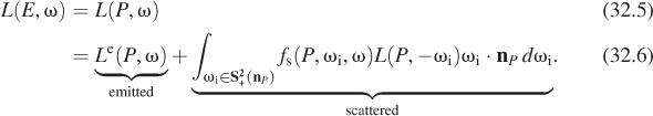
The rendering equation tells us that if P is the first point at which the ray t ![]() E – tω hits the geometry in the scene (see Figure 32.7), then
E – tω hits the geometry in the scene (see Figure 32.7), then
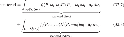
We can rewrite the second term as a sum by splitting the L in the integrand into two parts. As in Chapter 31, we let Lr = L – Le denote the reflected light (later, it will be reflected and refracted light) in the scene. At most surface points, Lr = L, because most points are not emitters. At emitters, however, Le is nonzero, so Lr and L differ. Thus,
Explain why, for a point Q on some luminaire and some direction ω, Lr(Q, ω) might be nonzero.
The first integral, representing scattered direct light, can be further expanded. We write ![]() as a sum of the illuminations due to the k individual luminaires, so that
as a sum of the illuminations due to the k individual luminaires, so that
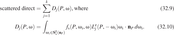
Thus, Dj(P, ω) represents the light reflected from P in direction ω due to direct light from source j.
Rather than computing Dj by integrating over all directions ωi in ![]() , we can simplify by integrating over only those directions where there’s a possibility that Le(P, –ωi) will be nonzero, that is, directions pointing toward the jth luminaire. We do so by switching to an area integral over the region Rj constituting the jth luminaire; the change of variables introduces the Jacobian we saw in Section 26.6.5:
, we can simplify by integrating over only those directions where there’s a possibility that Le(P, –ωi) will be nonzero, that is, directions pointing toward the jth luminaire. We do so by switching to an area integral over the region Rj constituting the jth luminaire; the change of variables introduces the Jacobian we saw in Section 26.6.5:
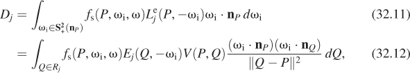
where ωi = S(Q – P) is the unit vector from P toward Q, and we have introduced the visibility term V(P, Q) in case the point Q is not visible from P. (Note that this transformation converts our version of the rendering equation into the form written by Kajiya [Kaj86].) The preceding argument only works for area luminaires. In the case of a point luminaire, this integral must be computed by a limit as in Chapter 31.
For an area luminaire, we estimate the integral with a single-sample Monte Carlo estimate:
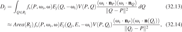
where Qj is a single point chosen uniformly with respect to area on the region Rj that constitutes the jth source.
The second integral, representing the scattering of indirect light, can also be split into two parts, by decomposing the function ωi ![]() fs(P, ωi, ω) in the integrand into a sum,
fs(P, ωi, ω) in the integrand into a sum,
where ![]() represents the impulses like mirror reflection (and later, Snell’s law transmission), and
represents the impulses like mirror reflection (and later, Snell’s law transmission), and ![]() is the nonimpulse part of the scattering distribution (i.e., fs is a real-valued function rather than a distribution). Each impulse can be represented by (1) a direction (the direction ωi such that –ωi either reflects or transmits to ω at P), and (2) an impulse magnitude 0 ≤ k ≤ 1, by which the incoming radiance in direction –ωi is multiplied to get the outgoing radiance in direction ω. We’ll index these by the letter m (where m = 1 is reflection and m = 2 is transmission). Thus, we can write
is the nonimpulse part of the scattering distribution (i.e., fs is a real-valued function rather than a distribution). Each impulse can be represented by (1) a direction (the direction ωi such that –ωi either reflects or transmits to ω at P), and (2) an impulse magnitude 0 ≤ k ≤ 1, by which the incoming radiance in direction –ωi is multiplied to get the outgoing radiance in direction ω. We’ll index these by the letter m (where m = 1 is reflection and m = 2 is transmission). Thus, we can write
Finally, we can again estimate that last integral—the diffusely reflected indirect light—by a single-sample Monte Carlo estimate: We pick a direction ωi according to some probability density on the hemisphere (or the whole sphere, when we’re considering refraction as well as reflection), and estimate the integral with
Note that while the BRDF doesn’t literally make sense for an impulse-like mirror reflection, the computation we perform to compute mirror-reflected radiance has a form remarkably similar to that of Equation 32.19. We wrote it (Equation 32.17) in the form
where ω1 was the reflection of ωi (ω2 was the transmitted direction). The coefficient k1 plays the same role as the coefficient
of the radiance in the current case. In each case, we simply need our representation of the BRDF to be able to return the appropriate coefficient.
32.5.2. Path-Tracer Code
The central code in the path tracer is shown in Listing 32.4.
Listing 32.4: The core procedure in a path tracer.
1 Radiance3 App::pathTrace(const Ray& ray, bool isEyeRay) {
2 // Compute the radiance BACK along the given ray.
3 // In the event that the ray is an eye-ray, include light emitted
4 // by the first surface encountered. For subsequent rays, such
5 // light has already been counted in the computation of direct
6 // lighting at prior hits.
7
8 Radiance3 L_o(0.0f);
9
10 SurfaceElement surfel;
11 float dist = inf();
12 if (m_world->intersect(ray, dist, surfel)) {
13 // this point could be an emitter...
14 if (isEyeRay && m_emit)
15 L_o += surfel.material.emit;
16
17 // Shade this point (direct illumination)
18 if ( (!isEyeRay) || m_direct) {
19 L_o += estimateDirectLightFromPointLights(surfel, ray);
20 L_o += estimateDirectLightFromAreaLights(surfel, ray);
21 }
22 if (!(isEyeRay) || m_indirect) {
23 L_o += estimateIndirectLight(surfel, ray, isEyeRay);
24 }
25 }
26
27 return L_o;
28 }
The broad strokes of this procedure match the path-tracing algorithm fairly closely. Not shown is the outer loop that, for each pixel in the image, creates a ray from the eye through that pixel and then calls the pathTrace procedure (perhaps doing so multiple times per pixel and taking a [possibly weighted] average of the results).
The computation consists of five parts: finding where the ray meets the scene (and storing the intersection in a SurfaceElement called surfel), and then summing up emitted radiance, radiance due to direct lighting from area lights, radiance due to direct lighting from point lights, and a recursive term, all evaluated at the intersection point. The inclusion of each term is governed by a flag (m_emit, m_direct, m_indirect) that lets us experiment with the program easily when we’re debugging. If we turn off direct and indirect light, it’s really easy to tell whether the lamps themselves look correct, for instance.
Let’s look at the four terms individually. The emissive term simply takes the emitted radiance at the surface point, called surfel.geometric.position in the code, but which we’ll call P in this description, and adds it to the computed radiance. This assumes that the surface is a Lambertian emitter so that the outgoing radiance in every direction from P is the same. If instead of having a constant outgoing radiance, the emitted radiance depended on direction, we might have written:
1 if (includeEmissive) {
2 L_o += surfel.material.emittedRadianceFunction(-ray.direction);
3 }
where the emitted radiance function describes the emission pattern. Notice that we compute the emission in the opposite of the ray direction; the ray goes from the eye toward the surface, but we want to know the radiance from the surface toward the eye.
We add to this emitted radiance the reflection of direct light (i.e., light that goes from a luminaire directly to P, and that scatters back along our ray), and the reflection of indirect light (i.e., all light leaving the intersection point that’s neither emitted light nor scattered direct light).
To compute the direct lighting from point lights (see Listing 32.5), we determine a unit vector w_i from the surface to the luminaire, and check visibility; if the luminaire is visible from the surface, we use w_i in computing the reflected light. This follows a convention we’ll use consistently: The variable w_i corresponds to the mathematical entity ωi; the letter “i” indicates “incoming”; the ray ωi points from the surface toward the source of the light, and ωo points in the direction along which it’s scattered. This means that the variable w_i will be the first argument to surfel,evaluateBSDF(...), and often a variable w_o will be the second argument. This convention matters: While the finite part of the BRDF is typically symmetric in its two arguments, both the mirror-reflectance and transmissive portions of scattering are often represented by nonsymmetric functions.
Listing 32.5: Reflecting illumination from point lights.
1 Radiance3 App::estimateDirectLightFromPointLights(
2 const SurfaceElement& surfel, const Ray& ray){
3
4 Radiance3 L_o(0.0f);
5
6 if (m_pointLights) {
7 for (int L = 0; L < m_world->lightArray.size(); ++L) {
8 const GLight& light = m_world->lightArray[L];
9 // Shadow rays
10 if (m_world->lineOfSight(
11 surfel.geometric.location + surfel.geometric.normal * 0.0001f,
12 light.position.xyz())) {
13 Vector3 w_i = light.position.xyz() - surfel.shading.location;
14 const float distance2 = w_i.squaredLength();
15 w_i /= sqrt(distance2);
16
17 // Attenuated radiance
18 const Irradiance3& E_i = light.color / (4.0f * pif() * distance2);
19
20 L_o += (surfel.evaluateBSDF(w_i, -ray.direction()) * E_i *
21 max(0.0f, w_i.dot(surfel.shading.normal)));
22 debugAssert(radiance.isFinite());
23 }
24 }
25 }
26 return L_o;
27 }
There are three slightly subtle points highlighted in the code. The first is that we don’t ask whether the luminaire is visible from the surface point; as we discussed earlier, we have to ask whether it’s visible from a slightly displaced surface point, which we compute by adding a small multiple of the surface normal to the surface-point location. The second is that we make sure that the direction from P to the luminaire and the surface normal at P point in the same hemisphere; otherwise, the surface can’t be lit by the luminaire. This test might seem redundant, but it’s not, for two reasons (see Figure 32.8). One is that the surface point might be at the very edge of a surface, and therefore be visible to a luminaire that’s below the plane of the surface. The other is that the normal vector we use in this “checking for illumination” step is the shading normal rather than the geometric normal. Since we actually compute the dot product with the shading normal, this can result in smoothly varying shading over a not-very-finely tessellated surface.
This is another general pattern: During computations of visibility, we’ll use the geometric data associated with the surface element. But during computations of light scattering, we’ll use surfel.shading.location. In general, our representation of the surface point has both geometric and shading data: The geometric data is that of the raw underlying mesh, while the shading data is what’s used in scattering computations. For instance, if the surface is displacement-mapped, the shading location may differ slightly from the geometric location. Similarly, while the geometric normal vector is constant across each triangular face, the shading normal may be barycentrically interpolated from the three vertex normals at the triangular face’s vertices.
The third subtlety is the computation of the radiance. As we discussed in Chapter 31, if we treat the point luminaire as a limiting case of a small, uniformly emitting spherical luminaire, the outgoing radiance resulting from reflecting this light is a product of a BRDF term, a cosine, and a radiance that varies with the distance from the luminaire; we called that E_i in the program. (We’ve also, as promised, ignored specular scattering of point lights.)
When we turn our attention to area luminaires (see Listing 32.6), much of the code is identical. Once again, we have a flag, m_areaLights, to determine whether to include the contribution of area lights. To estimate the radiance from the area luminaire, we sample one random point on the source, that is, we form a single-sample estimate of the illumination. Of course, this has high variance compared to sampling many points on the luminaire, but in a path tracer we typically trace many primary rays per pixel so that the variance is reduced in the final image. When testing visibility, we again slightly displace the point on the source as well as the point on the surface. Other than that, the only subtlety is in the estimation of the outgoing radiance. Since our light’s samplePoint samples uniformly with respect to area, we have to do a change of variables, and include not only the cosine at the surface point but also the corresponding cosine at the luminaire point, and the reciprocal square of the distance between them. By line 23, we’ve used these ideas to estimate the radiance from the area light scattered at P, except for impulse scattering, because evaluateBSDF returns only the finite portion of the BSDF.
At line 26 we take a different approach for impulse scattering: We compute the impulse direction, and trace along it to see whether we encounter an emitter, and if so, multiply the emitted radiance by the impulse magnitude to get the scattered radiance.
Listing 32.6: Reflecting illumination from area lights.
1 Radiance3 App::estimateDirectLightFromAreaLights(const SurfaceElement& surfel,
const Ray& ray){
2 Radiance3 L_o(0.0f);
3 // Estimate radiance back along ray due to
4 // direct illumination from AreaLights
5 if (m_areaLights) {
6 for (int L = 0; L < m_world->lightArray2.size(); ++L) {
7 AreaLight::Ref light = m_world->lightArray2[L];
8 SurfaceElement lightsurfel = light->samplePoint(rnd);
9 Point3 Q = lightsurfel.geometric.location;
10
11 if (m_world->lineOfSight(surfel.geometric.location +
12 surfel.geometric.normal * 0.0001f,
13 Q + 0.0001f * lightsurfel.geometric.normal)) {
14 Vector3 w_i = Q - surfel.geometric.location;
15 const float distance2 = w_i.squaredLength();
16 w_i /= sqrt(distance2);
17
18 L_o += (surfel.evaluateBSDF(w_i, -ray.direction()) *
19 (light->power()/pif()) * max(0.0f, w_i.dot(surfel.shading.normal))
20 * max(0.0f, -w_i.dot(lightsurfel.geometric.normal)/distance2));
21 debugAssert(L_o.isFinite());
22 }
23 }
24 if (m_direct_s) {
25 // now add in impulse-reflected light, too.
26 SmallArray<SurfaceElement::Impulse, 3> impulseArray;
27 surfel.getBSDFImpulses(-ray.direction(), impulseArray);
28 for (int i = 0; i < impulseArray.size(); ++i) {
29 const SurfaceElement::Impulse& impulse = impulseArray[i];
30 Ray secondaryRay = Ray::fromOriginAndDirection(
31 surfel.geometric.location, impulse.w).bumpedRay(0.0001f);
32 SurfaceElement surfel2;
33 float dist = inf();
34 if (m_world->intersect(secondaryRay, dist, surfel2)) {
35 // this point could be an emitter...
36 if (m_emit) {
37 radiance += surfel2.material.emit * impulse.magnitude;
38 }
39 }
40 }
41 }
42 }
43 return L_o;
44 }
At this point we’ve computed the emissive term of the rendering equation, and the reflected term, at least for light arriving at P directly from luminaires. We now must consider light arriving at P from all other sources, that is, light from some point Q that arrives at P having been reflected at Q rather than emitted. Such light is reflected at P to contribute to the outgoing radiance from P back toward the eye. Once again, we estimate this incoming indirect radiance with a single sample. To do so, we use our path-tracing code recursively. We build a ray starting at (or very near) P, going in some random direction ω into the scene; we use our path tracer to tell us the indirect radiance back along this ray, and reflect this, via the BRDF, into radiance transported from P toward the eye. Of course, in this case, we must not include in the computed radiance the light emitted directly toward P—we’ve already accounted for that. We therefore set includeEmissive to false at line 24. Listing 32.7 show this.
Listing 32.7: Estimating the indirect light scattered back along a ray.
1 Radiance3 App::estimateIndirectLight(
2 const SurfaceElement& surfel, const Ray& ray, bool isEyeRay){
3 Radiance3 L_o(0.0f);
4 // Use recursion to estimate light running back along ray
5 // from surfel, but ONLY light that arrives from
6 // INDIRECT sources, by making a single-sample estimate
7 // of the arriving light.
8
9 Vector3 w_o = -ray.direction();
10 Vector3 w_i;
11 Color3 coeff;
12 float eta_o(0.0f);
13 Color3 extinction_o(0.0f);
14 float ignore(0.0f);
15
16 if (!(isEyeRay) || m_indirect) {
17 if (surfel.scatter(w_i, w_o, coeff, eta_o, extinction_o, rnd, ignore)) {
18 float eta_i = surfel.material.etaReflect;
19 float refractiveScale = (eta_i / eta_o) * (eta_i / eta_o);
20
21 L_o += refractiveScale * coeff *
22 pathTrace(Ray(surfel.geometric.location, w_i).bumpedRay(0.0001f *
23 sign(surfel.geometric.normal.dot( w_i)),
24 surfel.geometric.normal), false);
25 }
26 }
27 return L_o;
28 }
The great bulk of the work is done in surfel.scatter(), which takes a ray r arriving at a point and either absorbs it or determines an outgoing direction r′ for it, and a coefficient by which the radiance arriving along r′ (i.e., the radiance L(P, –r′)) should be multiplied to generate a single-sample estimate of the scattered radiance at P in direction –r.
Before examining the scatter() code, let’s review that description more closely. First, scatter() can be used either in ray/path tracing or in photon tracing. The second use is perhaps more intuitive: We have a bit of light energy arriving at a surface, and it is either absorbed or scattered in one or more directions. The scatter() procedure is used to simulate this process. If the absorption at the surface is, say, 0.3, then 30% of the time scatter() will return false. The other 70% of the time it will return true and set the value of ωo. Given the direction ωi toward the source of the light, the probability of picking a particular direction ωo (at least for surfaces with no mirror terms or transmissive terms) for the scattered light is roughly proportional to fs(ωi, ωo). In an ideal world, it would be exactly proportional. In ours, it’s generally not, but the returned coefficient contains a fs(ωi, ωo)/p(ωo) factor, where p(ωo) is the probability of sampling ωo, which compensates appropriately.
What happens if there is a mirror reflection? Let’s say that 30% of the time the incoming light is absorbed, 50% of the time it’s mirror-reflected, and the remaining 20% of the time it’s scattered according to a Lambertian scattering model. In this situation, scatter() will return false 30% of the time. Fifty percent of the time it will return true and set ωo to be the mirror-reflection direction, and the remaining 20% of the time ωo will be distributed on the hemisphere with a cosine-weighted distribution (i.e., with high probability of being emitted in the normal direction and low probability of being emitted in a tangent direction).
Let’s see this in practice, and look at the start of G3D’s scatter method in Listing 32.8.
Listing 32.8: The start of the scatter method.
1 bool SurfaceElement::scatter
2 (const Vector3& w_i,
3 Vector3& w_o,
4 Color3& weight_o, // coeff by which to multiply sample in path-tracing
5 float& eta_o,
6 Color3& extinction_o,
7 Random& random,
8 float& density) const {
9
10 const Vector3& n = shading.normal;
11
12 // Choose a random number on [0, 1], then reduce it by each kind of
13 // scattering’s probability until it becomes negative (i.e., scatters).
14 float r = random.uniform();
15
16 if (material.lambertianReflect.nonZero()) {
17 float p_LambertianAvg = material.lambertianReflect.average();
18 r -= p_LambertianAvg;
19
20 if (r < 0.0f) {
21 // Lambertian scatter
22 weight_o = material.lambertianReflect / p_LambertianAvg;
23 w_o = Vector3::cosHemiRandom(n, random);
24 density = ...
25 eta_o = material.etaReflect;
26 extinction_o = material.extinctionReflect;
27 debugAssert(power_o.r >= 0.0f);
28
29 return true;
30 }
31 }
32 ...
As you can see, the material has a lambertianReflect member, which indicates reflectance in each of three color bands;2 the average of these gives a probability p of a Lambertian scattering of the incoming light. If the random value r is less than p, we produce a Lambertian-scattered ray; if not, we subtract that probability from r and move on to the next kind of scattering.
2. We’ll call these “red,” “green,” and “blue” in keeping with convention, but with no important change in the implementation, we could record five or seven or 20 spectral samples.
Convince yourself that this approach has a probability p of producing a Lambertian-scattered ray.
The actual scattering is fairly straightforward: The cosHemiRandom method produces a vector with a cosine-weighted distribution in the hemisphere whose pole is at n. The method also returns the index of refraction (both real and imaginary parts) of the material on the n side of the intersection point, and a coefficient, (called weight_o here) that is precisely the number we’ll need to use when we do Monte Carlo estimation of the reflected radiance. (The returned value density is not the probability density, but a rather different value included for the benefit of other algorithms, and we ignore it.)
The remainder of the scattering code is similar. Recall that the reflection model we’re using is a weighted sum of a Lambertian, a glossy component, and a transmissive component, where the weights sum to one or less. If they sum to less than one, there’s some absorption. The weights are specified for R, G, and B, and the sum must be no more than one in each component.
Listing 32.9: Further scattering code.
1 Color3 F(0, 0, 0);
2 bool Finit = false;
3
4 if (material.glossyReflect.nonZero()) {
5
6 // Cosine of the angle of incidence, for computing Fresnel term
7 const float cos_i = max(0.001f, w_i.dot(n));
8 F = computeF(material.glossyReflect, cos_i);
9 Finit = true;
10
11 const Color3& p_specular = F;
12 const float p_specularAvg = p_specular.average();
13
14 r -= p_specularAvg;
15 if (r < 0.0f) { // Glossy (non-mirror) case
16 if (material.glossyExponent != finf()) {
17 float intensity = (glossyScatter(w_i, material.glossyExponent,
18 random, w_o) / p_specularAvg);
19 if (intensity <= 0.0f) {
20 // Absorb
21 return false;
22 }
23 weight_o = p_specular * intensity;
24 density = ...
25
26 } else {
27 // Mirror
28
29 w_o = w_i.reflectAbout(n);
30 weight_o = p_specular * (1.0f / p_specularAvg);
31 density = ...
32 }
33
34 eta_o = material.etaReflect;
35 extinction_o = material.extinctionReflect;
36 return true;
37 }
38 }
The glossy portion of the model has an exponent that can be any positive number or infinity. If it’s infinity, then we have a mirror reflection; otherwise, we have a Blinn-Phong-like reflection, which is scaled by a Fresnel term, F. Listing 32.9 shows this code.
Finally, we compute the transmissive scattering due to refraction, with the code shown in Listing 32.10. The only subtle point is that the Fresnel coefficient for the transmitted light is one minus the coefficient for the reflected light.
Listing 32.10: Scattering due to transmission.
1 ...
2 if (material.transmit.nonZero()) {
3 // Fresnel transmissive coefficient
4 Color3 F_t;
5
6 if (Finit) {
7 F_t = (Color3::one() - F);
8 } else {
9 // Cosine of the angle of incidence, for computing F
10 const float cos_i = max(0.001f, w_i.dot(n));
11 // Schlick approximation.
12 F_t.r = F_t.g = F_t.b = 1.0f - pow5(1.0f - cos_i);
13 }
14
15 const Color3& T0 = material.transmit;
16
17 const Color3& p_transmit = F_t * T0;
18 const float p_transmitAvg = p_transmit.average();
19
20 r -= p_transmitAvg;
21 if (r < 0.0f) {
22 weight_o = p_transmit * (1.0f / p_transmitAvg);
23 w_o = (-w_i).refractionDirection(n, material.etaTransmit,
material.etaReflect);
24 density = p_transmitAvg;
25 eta_o = material.etaTransmit;
26 extinction_o = material.extinctionTransmit;
27
28 // w_o is zero on total internal refraction
29 return ! w_o.isZero();
30 }
31 }
32
33 // Absorbed
34 return false;
35 }
The code in Listing 32.10 is messy. It’s full of branches, and there are several approximations and apparently ad hoc tricks, like the Schlick approximation of the Fresnel coefficient, and the setting of the cosine of the incident angle to be at least 0.001, embedded in it. This is typical of scattering code. Scattering is a messy process, and we must expect the code to reflect this, but the messiness also arises from the challenges of floating-point arithmetic on machines of finite precision. Perhaps a more positive view is that the code will be called many times with many different parameter values, and it’s important that it be robust regardless of this wide range of inputs.
There is an alternative, however. If we actually know microgeometry perfectly, and we know the index of refraction for every material, we can compute scattering relatively simply—there’s a reflection term and a transmission term, and what’s neither reflected nor transmitted is absorbed. As long as the microgeometry is of a scale somewhat larger than the wavelength of light that we’re scattering, this provides a complete model. Unfortunately, at present it’s an impractical one, for several reasons. First, representing microgeometry at the scale of microfacets requires either an enormous amount of data or, if it’s generated procedurally, an enormous amount of computation. Second, if we accurately represent microgeometry, then every surface becomes mirrorlike at a small enough scale. To get the appearance of diffuse reflection at a point P requires that thousands of rays hit the surface near P, each scattering in its own direction. Ray-tracing a piece of chalk suddenly requires a thousand rays per pixel instead of just one! Third, the exact index of refraction for many materials is unknown or hard to measure, especially the coefficient of extinction.
Our representation of scattering by summary statistics like the diffuse coefficient is a way to take this intractable model and make it workable, with only slight losses in fidelity, based on the observation that the precise microgeometry almost never matters in the final rendering; if we render 20 pieces of chalk with the same macrogeometry, they’ll all look essentially identical.
There’s a third alternative between these two: You can store measured BRDF data. Storing such data, at a reasonably fine level of detail, can be expensive. (If your material has a glossy highlight that resembles the one produced by a Phong exponent of 1000, then the BRDF drops from its peak value to half that value in about 7°, suggesting that you might need to sample at least every 2° to faithfully capture it, requiring about 17,000 samples.) Drawing a direction ω with probability proportional to ω ![]() fs(ωi, ω) is far more problematic, but it is feasible. You might think that you could have the best of both worlds by choosing an explicit parametric representation (e.g., spherical harmonics, or perhaps some generalized Phong-like model) and finding the best fit to the measured data. This is a fairly common practice in the film industry today, and it works well for some materials like metals, but it can produce huge errors for diffuse surfaces when you use common analytic models that fail to model subsurface effects accurately [NDM05]. Nonetheless, it’s currently an active area of research, one with considerable promise for simplifying the computation of the scattering integral.
fs(ωi, ω) is far more problematic, but it is feasible. You might think that you could have the best of both worlds by choosing an explicit parametric representation (e.g., spherical harmonics, or perhaps some generalized Phong-like model) and finding the best fit to the measured data. This is a fairly common practice in the film industry today, and it works well for some materials like metals, but it can produce huge errors for diffuse surfaces when you use common analytic models that fail to model subsurface effects accurately [NDM05]. Nonetheless, it’s currently an active area of research, one with considerable promise for simplifying the computation of the scattering integral.
32.5.3. Results and Discussion
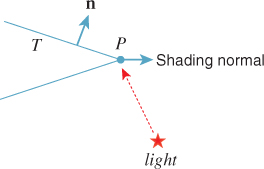
Figure 32.9 shows four simple scenes we’ll use in evaluating renderers, both drawn and ray-traced. The first, with its diffuse floor and back wall, and brightly colored semidiffuse sphere, provides a nice, simple test of bounding volume hierarchy, visibility, and rendering with reflection but not transmission. Since most of the scattering in the scene is diffuse, it only provides limited testing of scattering from multiple surfaces: We can’t visually check multiple interobject reflections the way we could in a scene with 12 mirrored spheres, for instance.
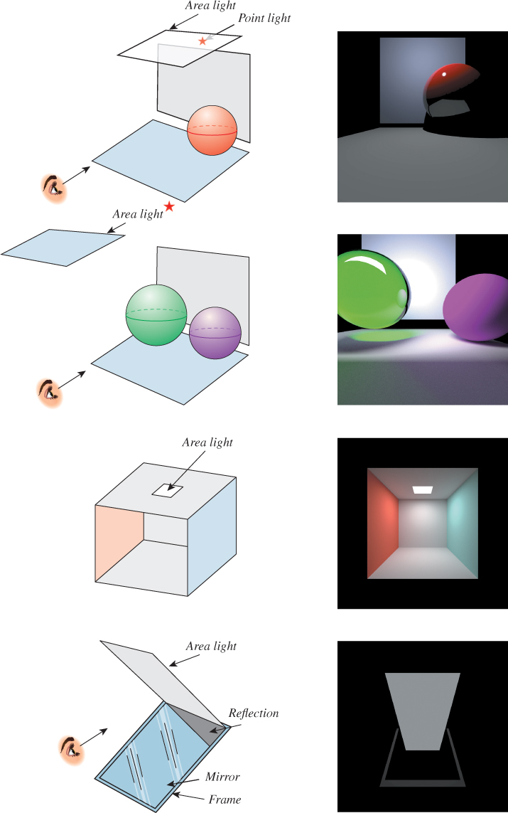
Figure 32.9: Four simple scenes, with their rendered versions shown to the right. The scene at the top is ray-traced (and hence the light comes from the point source; the area source is ignored); the three remaining scenes are path-traced to show the effects of the area luminaires.
In the second scene, we’ve added a transparent sphere whose refractive index is somewhat greater than that of air, to let us verify that transmissive scattering is working properly. (By the way, you can add a perfectly transmissive and completely nonreflective sphere with refractive index 1.0 to a scene, and it should make no difference to the scene’s appearance. Of course, if your renderer bounds the number of ray-surface interactions, it may have an effect on the rendering nonetheless.) The transparent sphere reflects some light from the other sphere, reflects some light onto it, and generates a diffuse pattern of light on the floor. None of these effects (color bleeding between diffuse surfaces, the caustic, or reflected light on the solid sphere) would be visible in a ray-traced version of the scene.
The third scene is the Cornell box, a standard test scene with diffuse surfaces, and an area light, in which color bleeding and multiple inter-reflections are evident in an accurate rendering, but are missing from the ray tracing.
The final scene consists of a large area light tilted toward the viewer, and a large mirror below it, also tilted toward the viewer, with a diffuse rectangle behind it to form a border for the mirror. The viewer sees not only the light, but also its reflection in the perfect mirror. Together these give the appearance of a single long continuous rectangle.
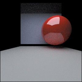
Figure 32.10 shows a path-traced version of the first scene. There are some obvious differences between this and the ray-traced scene. First, the area light, which we ignored in the ray tracing, has been included in the path tracing. Second, there’s noise in the path-traced image—everything looks somewhat speckled. We’ll return to this presently. Third, the shadows are softer. Light is reflecting from the floor onto the sphere, lighting the lower half somewhat, which in turn helps light the shadowed part of the floor. Fourth, there is color bleeding: The pinkish color on the floor and back wall is from light that’s reflected from the sphere.
The softened shadows and color bleeding are what you should expect when you consider how path tracing works. The noise, however, seems like a serious drawback. On the other hand, the ray-traced version exhibits aliasing, especially on the shadow edges. That’s because in the ray tracer, the rays from the eye through two nearby pixels end up reflecting from (or refracting through) the sphere in almost parallel directions. In the path tracer, there’s a coin toss: About 80% of the time a ray hitting the sphere, for instance, is reflected in a specific direction, and just as in ray tracing, nearby rays are refracted to nearby rays. But there’s also a 20% chance of absorption. If we trace, say, ten primary rays per pixel, it’s reasonable to expect seven, eight, nine, or ten of these rays to be reflected (i.e., from zero to four of them to be absorbed). That’ll lead to adjacent pixels having quite different radiance sums. To reduce this variance between adjacent pixels, we need to send quite a lot of primary rays (perhaps hundreds or thousands per pixel). You can even use the notion of confidence intervals from statistics to determine a number of samples so large that the fraction of absorbed rays is very nearly the absorption probability so that interpixel variation is small enough to be beneath the threshold of observation. In fact, Figure 32.10 was rendered with 100 primary rays per pixel, and despite this, the reflection of the floor in the red sphere appears slightly speckled. Figure 32.11 shows the speckle more dramatically.
32.6. Photon Mapping
Let’s now move on to a basic implementation of photon mapping. Recall that the main idea in photon mapping is to estimate the indirect light scattered from diffuse surfaces by shooting photons3 from the luminaires into the scene, recording where they arrive (and from what direction), and then reflecting them onward to be further recorded in subsequent bounces, eventually attenuated by absorption or by having the recursion depth-limited. When it comes time to estimate scattering at a point P of a diffuse surface, we search for nearby photons and use them as estimates of the arriving light at P, which we then push through the reflectance process to estimate the light leaving P.
3. Recall that a “photon” in photon mapping represents a bit of power emitted by the light, typically representing many physical photons.
Not surprisingly, much of the technology used in the path-tracing code can be reused for photon mapping. In our implementation, we have built a photon-map data structure based on a hash grid (see Chapter 37); as we mentioned in our discussion of photon mapping, any spatial data structure that supports rapid insertion and rapid neighborhood queries can be used instead.
We’ve defined two rather similar classes, EPhoton and IPhoton, to represent photons as they are emitted and when they arrive; the “I” in IPhoton stands for “incoming.” An EPhoton has a position from which it was emitted, and a direction of propagation, which are stored together in a propagation ray, and a power, representing the photon’s power in each of three spectral bands. An IPhoton, by contrast, has a position at which it arrived, a direction to the photon source from that position, and a power. Making distinct classes helps us keep separate the two distinct ways in which the term “photon” is used. In our implementation, an EPhoton is emitted, and its travels through the scene result in one or more IPhotons being stored in the photon map.
The basic structure of the code is to first build the photon map, and then render the scene using it. Listing 32.11 shows the building of the photon map: We construct an array ephotons of photons to be emitted, and then emit each into the scene to generate an array iphotons of incoming photons, and store these in the map m_photonMap.
Listing 32.11: The large-scale structure of the photon-mapping code.
1 main(){
2 set up image and display, and load scene
3 buildPhotonMap();
4 call photonRender for each pixel
5 display the resulting image
6 }
7
8 void App::buildPhotonMap(){
9 G3D::Array<EPhoton> ephotons;
10 LightList lightList(&(m_world->lightArray), &(m_world->lightArray2), rnd);
11 for (int i = 0; i < m_nPhotons; i++) {
12 ephotons.append(lightList.emitPhoton(m_nPhotons));
13 }
14
15 Array<IPhoton> ips;
16 for (int i = 0; i < ephotons.size(); i++) {
17 EPhoton ep = ephotons[i];
18 photonTrace(ep, ips);
19 m_photonMap.insert(ips);
20 }
21 }
The LightList represents a collection of all point lights and area lights in the scene, and can produce emitted photons from these, with the number of photons emitted from each source being proportional to the power of that source. Listings 32.12 and 32.13 show a little bit of how this is done: We sum the power (in the R, G, and B bands) for each light to get a total power emitted. The probability that a photon is emitted by the ith light is then the ratio of its average power (over all bands) to the average of the total power over all bands. These probabilities are stored in an array, with one entry per luminaire.
Listing 32.12: Initialization of the LightList class.
1 void LightList::initialize(void)
2 {
3 // Compute total power in all spectral bands.
4 foreach point or area light
5 m_totalPower += light.power() //totalPower is RGB vector
6
7 // Compute probability of emission from each light
8 foreach point or area light
9 m_probability.append(light.power().average() / m_totalPower.average());
10 }
With these probabilities computed, the only subtlety remaining is selecting a random point on the surface of an area light (see Listing 32.13). If the area light has some known geometric shape (cube, sphere, ...), we can use the obvious methods to sample from it (see Exercise 32.12). On the other hand, if it’s represented by a triangle mesh, we can first pick a triangle at random, with the probability of picking a triangle T proportional to the area of T, and then pick a point in that triangle uniformly at random. Exercise 32.6 shows that generating samples uniformly on a triangle may not be as simple as you think.
The areaLightEmit code uses cosHemiRandom to generate a photon in direction (x, y, z) with probability cos(θ), where θ is the angle between (x, y, z) and the surface normal. Why?
Listing 32.13: Photon emission in the LightList class.
1 // emit a EPhoton; argument is total number of photons to emit
2 EPhoton LightList::emitPhoton(int nEmitted)
3 {
4 u = uniform random variable between 0 and 1
5 find the light i with p0 + ... + pi-1 ≤ u < p0 + ... + pi.
6 if (i < m_nPointLights)
7 return pointLightEmit((*m_pointLightArray)[i], nEmitted, m_probability[i]);
8 else
9 return areaLightEmit((*m_areaLightArray)[i - m_nPointLights], nEmitted,
10 m_probability[i]);
11 }
12
13 EPhoton LightList::pointLightEmit(GLight light, int nEmitted, float prob){
14 // uniformly randomly select a point (x,y,z) on the unit sphere
15 Vector3 direction(x, y, z);
16 Power3 power = light.power() / (nEmitted * prob);
17 Vector3 location = location of the light
18 return EPhoton(location, direction, power);
19 }
20
21 EPhoton LightList::areaLightEmit(AreaLight::Ref light, int nEmitted, float prob){
22 SurfaceElement surfel = light->samplePoint(m_rnd);
23 Power3 power = light->power() / (nEmitted * prob);
24 // select a direction with cosine-weighted distribution around
25 // surface normal. m_rnd is a random number generator.
26 Vector3 direction = Vector3::cosHemiRandom(surfel.geometric.normal, m_rnd);
27
28 return EPhoton(surfel.geometric.location, direction, power);
29 }
What remains is the photon tracing itself (see Listing 32.14). We use a G3D helper class, the Array<IPhoton>, to accumulate incident photons. This class has a fastClear method that simply sets the number of stored values to zero rather than actually deallocating the array; this saves substantial allocation/deallocation overhead. The photonTraceHelper procedure keeps track of the number of bounces that the photon has undergone so far so that the bounce process can be terminated when this reaches the user-specified maximum. Note that in contrast to Jensen’s original algorithm, we store a photon at every bounce, whether it’s diffuse or specular. For estimating radiance at surface points with purely impulsive scattering models (e.g., mirrors), these photons will never be used, however, so there’s no impact on the results.
Once again, there are no real surprises in the program. The scatter method does all the work. We’ve hidden one detail here: The scatter method should be different from the one used in path tracing. If we’re only studying reflection, and only using symmetric BRDFs (i.e., all materials satisfy Helmholtz reciprocity), then the two scattering methods are the same. But in the case of asymmetric scattering (such as Fresnel-weighted transmission), it’s possible that the probability that a photon arriving at P in direction ωi scatters in direction ωo is completely different from the probability that one arriving in direction ωo scatters in direction ωi. Our surface really needs to provide two different scattering methods, one for each situation. In our code, we’ve used the same method for both. That’s wrong, but it’s also very common practice, in part because the effects of making the code right are (a) generally small, and (b) generally not something we’re perceptually sensitive to. You might want to spend a little while trying to imagine a scene in which the distinction between the two scattering rules matters.
Listing 32.14: Tracing photons, which is rather similar to tracing rays or paths.
1 void App::photonTrace(const EPhoton& ep, Array<IPhoton>& ips) {
2 ips.fastClear();
3 photonTraceHelper(ep, ips, 0);
4 }
5
6 /**
7 Recursively trace an EPhoton through the scene, accumulating
8 IPhotons at each diffuse bounce
9 */
10 void App::photonTraceHelper(const EPhoton& ep, Array<IPhoton>& ips, int bounces) {
11 // Trace an EPhoton (assumed to be bumped if necessary)
12 // through the scene. At each intersection,
13 // * store an IPhoton in "ips"
14 // * scatter or die.
15 // * if scatter, "bump" the outgoing ray to get an EPhoton
16 // to use in recursive trace.
17
18 if (bounces > m_maxBounces) {
19 return;
20 }
21
22 SurfaceElement surfel;
23 float dist = inf();
24 Ray ray(ep.position(), ep.direction());
25
26 if (m_world->intersect(ray, dist, surfel)) {
27 if (bounces > 0) { // don’t store direct light!
28 ips.append(IPhoton(surfel.geometric.location, -ray.direction(), ep.power()));
29 }
30 // Recursive rays
31 Vector3 w_i = -ray.direction();
32 Vector3 w_o;
33 Color3 coeff;
34 float eta_o(0.0f);
35 Color3 extinction_o(0.0f);
36 float ignore(0.0f);
37
38 if (surfel.scatter(w_i, w_o, coeff, eta_o, extinction_o, rnd, ignore)) {
39 // managed to bounce, so push it onwards
40 Ray r(surfel.geometric.location, w_o);
41 r = r.bumpedRay(0.0001f * sign(surfel.geometric.normal.dot( w_o)),
42 surfel.geometric.normal);
43 EPhoton ep2(r, ep.power() * coeff);
44 photonTraceHelper(ep2, ips, bounces+1);
45 }
46 }
47 }
One difference between photon propagation and radiance propagation is that at the interface between media with different refractive indices, the radiance changes (because a solid angle on one side becomes a different solid angle on the other), while for photons, which represent power transport through the scene, there is no such change. Thus, there’s no ηi/ηo factor in the photon-tracing code.
Having built the photon map, we must render a picture based on it. Our first version will closely resemble the path-tracing code, in the sense that we’ll break up the computation into direct and indirect light, and handle diffuse and impulse scattering individually. We’ll use a ray-tracing approach (i.e., recursively trace rays until some fixed depth); making the corresponding path-tracing approach is left as an exercise for the reader. The photon map is used only to estimate the diffusely reflected indirect light arriving at a point.
Computing the light arriving at pixel (x, y) of the image, using a ray-tracing and photon-mapping hybrid, is the job of the photonRender procedure, shown in Listing 32.15, along with some of the methods it calls.
Listing 32.15: Generating an image sample for pixel (x, y) from the photon map.
1 void App::photonRender(int x, int y) {
2 Radiance3 L_o(0.0f);
3 for (int i = 0; i < m_primaryRaysPerPixel; i++) {
4 const Ray r = defaultCamera.worldRay(x + rnd.uniform(),
5 y + rnd.uniform(), m_currentImage->rect2DBounds());
6 L_o += estimateTotalRadiance(r, 0);
7 }
8 m_currentImage->set(x, y, L_o / m_primaryRaysPerPixel);
9 }
10
11 Radiance3 App::estimateTotalRadiance(const Ray& r, int depth) {
12 Radiance3 L_o(0.0f);
13 if (m_emit) L_o += estimateEmittedLight(r);
14
15 L_o += estimateTotalScatteredRadiance(r, depth);
16 return L_o;
17 }
18
19 Radiance3 App::estimateEmittedLight(Ray r){
20 ...declarations...
21 if (m_world->intersect(r, dist, surfel))
22 L_o += surfel.material.emit;
23 return L_o;
24 }
To generate a measurement at pixel (x, y) we shoot m_primaryRaysPerPixel into the scene, and estimate the radiance returning along each ray. It’s possible that a ray hits a light source; if so, the source’s radiance (EmittedLight) must be counted in the total radiance returning along the ray, along with any light reflected from the luminaire.
We’ve ignored the case where the ray hits a point luminaire (point sources have no geometry in our scene descriptions, so such an intersection is never reported). There are two reasons for this. The first is that the intersection of the ray and the point light is an event with (mathematical) probability zero, so in an ideal program with perfect precision, it should never occur. This is a frequently used but somewhat specious argument: First, the discrete nature of floating-point numbers makes probability-zero events occur with very small, but nonzero, frequency. Second, models like point-lighting are usually taken as a kind of “limit” of nonzero-probability things (like small, disk-shaped lights); if the limit is to make any sense, the effect of the limiting case should be the limit of the effects in the nonlimiting cases. If the disk-shaped lights are given values that increase with the inverse square of the radius, then these nonlimiting cases may produce nonzero effects, which should show up in the limiting case as well.
The other, far more practical, reason for not letting rays hit point lights is that point lights are an abstract approximation to reality, used for convenience, and if you want them to be visible in your scene you can model them as small spherical lights. In our test cases, there are no point lights visible from the eye, so the issue is moot.
In general, not only might light be emitted by the place where the ray meets the scene, but also it may be scattered from there as well. The estimateTotalScatteredRadiance procedure handles this (see Listing 32.16) by summing up the direct light, impulse-scattered indirect light, and diffusely reflected direct light.
Listing 32.16: Estimating the total radiance scattered back toward the course of the ray r.
1 Radiance3 App::estimateTotalScatteredRadiance(const Ray& r, int depth){
2 ...
3 if (m_world->intersect(r, dist, surfel)) {
4 L_o += estimateReflectedDirectLight(r, surfel, depth);
5 if (m_IImp || depth > 0) L_o +=
6 estimateImpulseScatteredIndirectLight(r, surfel, depth + 1);
7 if (m_IDiff || depth > 0) L_o += estimateDiffuselyReflectedIndirectLight(r, surfel);
8 }
9 return L_o;
10 }
In each case, there’s a Boolean control for whether to include this aspect of the light. We’ve chosen to apply this control only to the first reflection (i.e., if m_IImp is false, then impulse-scattered indirect light is ignored only when it goes directly to the eye).
Listing 32.17: Impulse-scattered indirect light.
1 Radiance3 App::estimateImpulseScatteredIndirectLight(const Ray& ray,
2 const SurfaceElement& surfel, int depth){
3 Radiance3 L_o(0.0f);
4
5 if (depth > m_maxBounces) {
6 return L_o;
7 }
8
9 SmallArray<SurfaceElement::Impulse, 3> impulseArray;
10
11 surfel.getBSDFImpulses(-ray.direction(), impulseArray);
12 foreach impulse
13 const SurfaceElement::Impulse& impulse = impulseArray[i];
14
15 Ray r(surfel.geometric.location, impulse.w);
16 r = r.bumpedRay(0.0001f * sign(surfel.geometric.normal.dot( r.direction())),
17 surfel.geometric.normal);
18 L_o += impulse.magnitude* estimateTotalScatteredRadiance(r, depth + 1);
19
20 return L_o;
21 }
The direct-lighting computation is essentially identical to that in the path tracer, except that we estimate the direct light from each area light with several (m_diffuseDirectSamples) samples rather than relying on multiple primary rays to ensure adequate sampling. (The alternative is quite viable, however.) The similarity is so great that we omit the code. This leaves only the impulse-scattered and diffusely reflected indirect light to consider. The first is easy, and it closely resembles the corresponding path-tracing code: We simply compute the total arriving radiance for each impulse recursively, and sum (see Listing 32.17).
This leaves only the computation of diffusely reflected indirect light, which is where the photon map finally comes into play (see Listing 32.18). Central to this code is the photon map’s kernel, the function that says how much weight to give each nearby photon’s contribution.
Listing 32.18: The photon map used to compute diffusely reflected indirect light.
1 Radiance3 App::estimateDiffuselyReflectedIndirectLight(const Ray& r,
2 const SurfaceElement& surfel){
3 Radiance3 L_o(0.0f);
4 Array<IPhoton> photonArray;
5 // find nearby photons
6 m_photonMap.getIntersectingMembers(
7 Sphere(surfel.geometric.location, m_photonMap.gatherRadius()), photonArray);
8
9 foreach photon p in the array
10 const float cos_theta_i =
11 L_o += p.power() * m_photonMap.kernel(p.position(), surfel.shading.location) *
12 surfel.evaluateBSDF(p.directionToSource(), -r.direction(), finf());
13 return L_o;
14 }
We sum up the contributions of all sufficiently nearby photons, weighting them by our kernel and pushing each one through the BSDF to determine the light it contributes traveling toward the source of the ray r.
Note that what is being multiplied by the BRDF term is an area-weighted radiance, which is what we called biradiance in Chapter 14.
32.6.1. Results and Discussion
Naturally, as we discussed in Chapter 31, there’s an interaction between the gather radius, the number of photons stored in the photon map, and the quality of the estimated radiance. When we’re estimating the reflected indirect radiance at P, if we use a cylinder kernel (a photon is counted if it’s within some distance of P, and ignored otherwise) and there are no photons within the gather radius of P, the radiance estimate for that ray will be zero. This can happen if the gather radius is too small or if there are too few photons. How many photons are enough? Well, we’d generally like nearby pixel rays hitting the same surface to get similar radiance estimates. But one ray might be within the radius of 20 photons, while the nearby ray might be within the radius of 21 photons. Even if all the photons share the same incoming power, the second ray will get a radiance that’s 5% greater. To reduce the noise in areas of constant radiance, it appears that we might need hundreds of photons within the gather radius of P.
There are several ways to improve the results without needing that many photons. One is to alter the photon map’s kernel—the weighting function, centered at P, that determines how much each photon’s contribution should matter in the radiance estimate. If we change from the cylinder kernel to a conelike function (photons near the gather radius have their contributions reduced to near zero), then each arrival or departure of a photon within the gather radius (as we vary P) has a gradual impact. This is the approach used in our renderer.
A very different approach is described by Jensen: Rather than gathering photons within a fixed radius, we enlarge the radius enough to get a certain number of photons, and then use the area of the resultant disk in the conversion from power (stored at incoming photons) to outgoing radiance.
The ray-trace-with-photon-mapping renderer we’ve written has several parameters (the number of samples to use to estimate lighting from area lights, the radius of the kernel, the number of photons to shoot into the scene), each of which has an effect on the final result. Figure 32.12 shows that with only 100 photons, the Cornell box scene looks blotchy, because most points in the scene are not within the kernel radius of any photons at all. With one million photons, each point is near thousands of photons, and the estimate of diffusely reflected indirect light is very smooth. (We’ve used a large number of samples for area lights to reduce that source of variation in the image.)
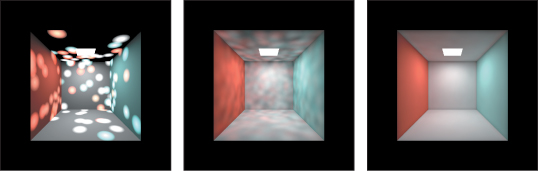
With a larger kernel radius, the low-photon-count image would look smoother, but then distant photons would affect the appearance of the scene at any point. Clearly there’s a tradeoff between photon count N and kernel radius r. In Jensen’s original photon-mapping algorithm, the radiance estimate was provided by using a fixed number, k, of photons, enlarging the radius as necessary to find that many photons. This has the advantage of scale invariance—if you double the scene size, you needn’t change anything—but it still leaves the problem of choosing N and k.
The number of samples used in estimating direct lighting from area lights also has an impact on noise in the image. Figure 32.13 shows this, again using the Cornell box. With only one sample per light, the image is very noisy; with 100, the noise is lower than that of the photon-mapped estimate of reflected indirect radiance in Figure 32.12.
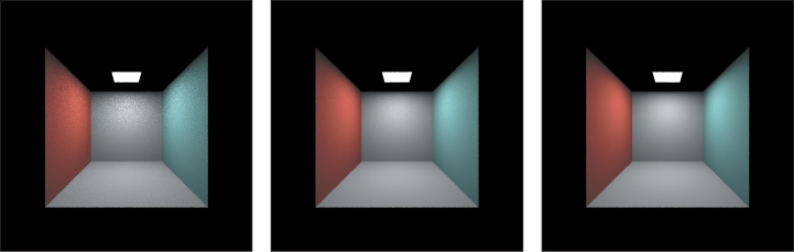
Figure 32.13: One-sample-per-pixel rendering of the emitted direct light from area lights only, using 1, 10, and 100 samples to estimate the light from the area source.
In the one-sample-per-source image, how is the noisiness correlated with the brightness, and why? In which areas of the image is the human visual system most sensitive to the noise?
It’s typical in renderers like this one to use many primary rays per pixel. If we use 100 primary rays, then we need not use very many rays (per primary ray) to estimate direct lighting from area sources. We still, however, as Inline Exercise 32.8 shows, must address the noise in some way, particularly if there are dark areas in the scene. Fortunately in the case of the Cornell box, indirectly reflected light dominates the direct light near the top, and so the noise there ends up less perceptually significant when we include indirect light.
Looking at the other test scenes (see Figure 32.14), we see that photon mapping with one million photons handles the first scene very well. The third scene, with the transparent sphere, exhibits a caustic highlight beneath the sphere. In the fourth scene, the emitting luminaire is (as a reflector) completely Lambertian and black. The mirror is pure specular, and the panel beneath the mirror is dark and Lambertian. Even with one million photons shot, only a few photons end up in the scene, and they’re used only in estimating the brightness of the panel beneath the mirror, which is overwhelmingly determined by direct lighting, so the computation of the photon map was almost pointless.
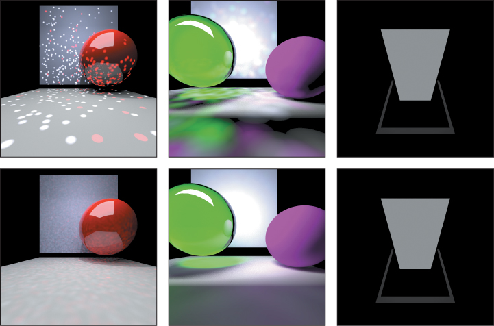
Figure 32.14: The three other test scenes, rendered with 100 primary rays per pixel, ten thousand (top row) and one million (bottom row) shot photons, and one sample per source for area lights.
In all versions of photon mapping, we’re converting from samples of the arriving power near P to an estimate of that power at P. This is extremely closely related to the problem of density estimation in statistics. The most basic form of density estimate is nearest neighbor, in which the value at P is taken to be the value at the sample nearest to P. For a continuous density, this converges to the correct value as the number of samples gets large, but the convergence is not exactly the kind we’d like: For any fixed set of samples, the nearest-neighbor estimate of density is piecewise-constant. (On a plane, the regions of constancy are the Voronoi cells associated to the samples.) This leads to a great many discontinuities. On the other hand, as the number of samples increases, the values in adjacent cells get closer and closer, so while the set of discontinuities grows, the magnitude of the discontinuities decreases [WHSG97].
There are many other forms of density estimation aside from nearest-neighbor interpolation. Weighted averaging by some filter kernel is one; Jensen’s method of gathering a fixed number of samples and then dividing by a value that depends on those samples is another. Whole books have been written on density estimation, and the statistics and mathematics quickly become increasingly complex as the sophistication of the methods increases.
32.6.2. Further Photon Mapping
The hybrid ray-tracing-photon-mapper approach described above is very basic. Just as we factored out direct lighting, computing it with ray-tracing rather than the photon map, it’s possible to build special photon maps that contain only photons that have passed through particular sequences of scattering, such as caustics and shadows (carefully omitting these photons from the generic photon map so that they’re not double-counted). Such specialized maps can be used to more accurately generate such phenomena, at the cost of ever-growing code complexity.
There is one technique, however, that applies not just to photon mapping, but to many algorithms: a final gather step, in which the incoming radiance at the eye-ray/scene-intersection point is estimated by tracing several rays from that intersection and using some estimation technique at the secondary intersections to determine the radiance along those rays; these secondary estimates are then combined to form an estimate along the eye ray. For instance, if the eye ray meets the world at P, we trace 20 rays from P that meet the world at locations Q1, ..., Q20. At each Qi, we can use our photon map to estimate the radiance leaving Qi in the direction toward P, and then combine these 20 samples of arriving radiance at P to get the radiance exiting from P toward the eye. By carefully selecting the directions along which to sample, we can produce an estimate of the outgoing radiance at P that has far fewer artifacts than would arise from the direct photon-map estimate. For instance, if the photon map is using a disk-shaped reconstruction filter, and not very many photons, there will be many sharp discontinuities in the reconstructed radiance estimates used at the points Qi. But when these are averaged by the reflectance equation at P to produce the outgoing radiance there, the result is far fewer artifacts in the final rendering.
The alteration in the code is quite minor, as shown in Listing 32.19: The code for estimating the diffusely reflected indirect light at the point P gets a new argument—useGather—that is set to true for primary rays but false for all subsequent ones. When it’s false, we use the photon map as above. But when it’s true, we essentially perform one-level ray tracing, with a large number of secondary rays, using photonRender to estimate the incoming radiance along these.
Listing 32.19: Using final gathering to improve the estimate of indirect radiance arriving at a point.
1 Radiance3 App::estimateDiffuselyReflectedIndirectLight(..., boolean useGather)
2 // estimate arriving radiance at "surfel" with final gather.
3 Radiance3 L(0.0f);
4
5 if (!useGather)
6 ... use the previous photon-mapping code and return radiance ...
7 else {
8 for (int i = 0; i < m_gatherRaysPerSample; i++) {
9 // draw a cosine-weighted sample direction from the surface point
10 Vector3 w_i = -r.direction();
11 Vector3 w_o = Vector3::cosHemiRandom(surfel.geometric.normal, rnd);
12 Ray gatherRay = Ray(surfel.geometric.location, w_o).bumpedRay(...)
13
14 Color3 coeff;
15 L += π * surfel.evaluateBSDF(w_i, w_o, finf()) *
16 estimateTotalScatteredRadiance(gatherRay, depth+1, false);
17 }
18 }
19 return L / m_gatherRaysPerSample;
20 }
The improvement in results is dramatic, at least if we’re willing to use a large number of rays in our final gathering. If we’re typically averaging contributions from 20 nearby photons in the nongather version of the code, we should be using at least 20 gather rays to estimate the radiance in the gather version. Figure 32.15 shows the effect of the final gather.
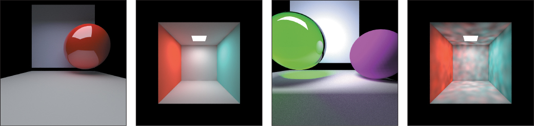
Figure 32.15: Final gathering with 30 samples in our first three test scenes. The photon maps were generated with 10,000 shot photons, resulting in 1,100 photons (first scene) to 7,900 photons (second scene). The last image is the Cornell box, rendered with the same parameters but no final gather. The improvement is substantial.
32.7. Generalizations
Because photon mapping provides a consistent estimate of reflected indirect radiance, we can take any rendering algorithm that needs such an estimate (ray tracing, path tracing) and replace its estimator with a photon-mapping implementation. A similar argument allows one to replace direct evaluation by a final-gather step. Similarly, it’s possible to break up the rendering integral into various pieces (as we did for impulse-scattered indirect light, diffusely scattered direct light, etc.), and estimate each part separately. In some cases, direct evaluation rather than estimation is possible (e.g., mirror reflection of direct light from area lights); removing this component of the integrand makes the remaining scattered light a smoother function of the outgoing direction and/or the scattering location, and thus allows better stochastic estimation with fewer samples.
Certain classes of illumination and reflection are amenable to particular approaches. For instance, it’s very difficult to use Monte Carlo methods based on ray tracing from the eye to render a scene that’s lit by tiny luminaires: The chance that a ray (primary or scattered) will hit the light is so small that the variance in the radiance estimate ends up large. On the other hand, if we trace rays from the luminaire to build up a photon map, it becomes easy to estimate the diffusely scattered radiance from small sources, or even scattering along light paths of the form LS+DE. A dual situation is the rendering of area lights that are multiply scattered by highly specular surfaces. It’s very difficult to pick a point of such a light, and a direction for emission, with the property that the resultant light path eventually reaches the eye. Such a situation is far more amenable to ray tracing. To handle both cases, you find you want to trace both from the eye and from luminaires, and you’re in the realm of bidirectional path tracing [LW93, Vea97]. Whether you choose to glue paths together or use a density-estimation strategy like photon mapping depends on the classes of paths you encounter. In fact, it’s natural to begin thinking that for each possible path type, you might want to choose different ways of working with those paths, and then combine the results at the end. Choosing a reasonable way to combine the multiple sampling approaches (or, thinking in the opposite direction, a reasonable way to break up the integrand or domain of integration) leads quite naturally to methods similar to those used for Metropolis light transport.
Broadly speaking, there’s a whole collection of possible approaches that you can take in building a rendering algorithm, and you can put the pieces together in many different ways. Considerations of classes of phenomena that are important to you (caustics, shadows) may make one method preferable over another. Considerations of efficiency, either in the big-O running time of a procedure, or in coherence of memory access or careful use of bandwidth, may also be an influence. Don’t be constrained by what others have done: Evaluate the specific rendering problem you need to solve, and then combine techniques as necessary to optimize.
32.8. Rendering and Debugging
In Chapter 5 we discussed how very sensitive the human visual system can be to certain kinds of artifacts in images. Renderers give you the opportunity to put that sensitivity to work. Not only do they provide millions of parallel executions of the same bit of code (typically one or more executions per image pixel), but it’s easy to construct scenes that have a natural coherence to them so that any anomaly stands out.
Let’s look at several examples to see how you can debug a renderer. Suppose you’re writing a path tracer, and you find that increasing the number of primary rays causes the image to get dimmer, but does not improve the aliasing artifacts around shadows. The dimming of the image suggests that you’re dividing by the number of primary rays, as you should, but that you’re failing to accumulate radiance in proportion to the number of primary rays. Probably the part of your code shown in Listing 32.20 has L = estimateTotalRadiance(...) rather than L += estimateTotalRadiance(...). That accounts for the presence of the aliasing artifacts: You’re still working with only one sample per pixel!
Listing 32.20: Averaging several primary rays.
1 for (int i = 0; i < m_primaryRaysPerPixel; i++) {
2 const Ray r = defaultCamera.worldRay(x + rnd.uniform(), y + rnd.uniform(),..)
3 L += estimateTotalRadiance(r, 0);
4 }
5 m_currentImage->set(x, y, L / m_primaryRaysPerPixel);
Suppose, on the other hand, that increasing the number of primary samples causes the image to grow brighter. Then perhaps you’re accumulating radiance, but failing to divide by the number of primary rays.
Now suppose that your objects mostly look good, but one sphere seems to be missing its left third—you can see right through where that part of the sphere should be. What could be wrong? Well, that’s a failure to correctly compute the intersection of a ray with the world, so it’s got to be a problem with the bounding volume hierarchy (BVH) if you’re using one. The fact that it looks as if the sphere was chopped off by a plane suggests that some bounding-plane test is failing. Perhaps switching to a different BVH will get you the correct results, and thus help you diagnose the problem in the BVH code. By the way, if some plane has just a single line of pixels that you can see through (or perhaps a line where you see through just a few of the pixels), it suggests a failure of a floating-point comparison: Perhaps one side of a dividing plane is using a less-than test while the other is using a greater-than test, and the few pixels where the test reveals equality aren’t handled by either side of the plane (see Figure 32.16).
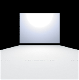
Most Monte Carlo rendering approaches produce high-variance results when you have relatively few samples per pixel. But if you render a Cornell box, for instance, then a typical secondary ray will hit one of the sides of the box, all of which are of comparable brightness. Sure, a ray could go into one of the dark corners, and some rays will come out of the front of the box into empty space. But in general, if there are a few secondary rays per pixel, the resultant appearance should be fairly smooth. If you find yourself confronting a “speckled” rendering like the one shown in Figure 32.17 (produced with one primary ray per pixel) you’re probably confronting a visibility problem. For contrast, Figure 32.18 shows the same rendering with the visibility problem fixed; there’s still lots of noise from the stochastic nature of the path tracer, but no really dark pixels.
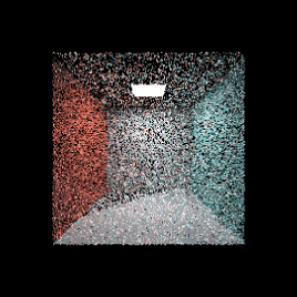
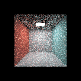
The path for diagnosis is relatively simple. If you eliminate all but direct lighting and still have speckles, then some rays from the hit point to the area-light point must be failing their visibility test. There are two possibilities. The first is that perhaps the points generated on the area light are actually not visible. If you’ve made a small square hole in the ceiling and placed a large square light slightly above it, then many random light points won’t be visible from the interior. This is just a modeling mistake. On the other hand, perhaps the light-sampling code has a bug, and the light points being generated do not actually lie on the light itself. The other possibility is that the hit point and light point really are not visible from each other because of a failure to bump one or both. Figure 32.17 was generated by removing the bumpedRay calls in the path tracer, for instance. The failure of an unbumped ray to see some other point is typically the result of some floating-point computation going wrong: A number you expected to be slightly greater than zero was in fact slightly less. The dependence of this error on the point locations is likely to be tied to the floating-point representation, and to generate random results like speckle. But sometimes there’s a strong enough dependence on a single parameter that there’s regularity in the results. Figure 32.19 shows how the floor of the Cornell box is irregularly illuminated (a triangle in the back-right corner is too dark) when we fail to bump just the light-point position.
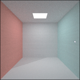
Suppose that your photon mapper shows nice, smooth gradations of reflected light in the Cornell box, but there’s no color bleeding: The left side of the floor isn’t slightly red and the right side isn’t slightly blue. Think for a moment about what might be wrong, and then read on.
One thing to ask is, “Are the photons correct?” You can plot each photon as a point in your scene to verify that they’re well scattered, and you can even plot each one as a small arrow whose base is at the photon location, and which points toward the source of the light. If all the photons point toward the area light, there’s a problem: You’re not getting any scattered photons in your photon map. (You’re also storing first-hit photons, which may be intentional, but if you’re computing direct illumination in a separate step, as we did, it’s a mistake: You’ll end up double-counting the direct illumination!) Interpolating values from the photons you have will tend to give smoothly varying light, however. But you won’t get color bleeding. Let’s assume, though, that the photons are well scattered, only store indirect light, and seem to get their indirect light from many different places.
A photon on the floor near the red wall probably got there by having light hit the red wall and reflect to the floor. The problem has to be in the reflection process, that is, the multiplication by the BRDF and a cosine. Since the magnitude looks right, the absorption/reflection part of the code must be right. But the spectral distribution of the outgoing photon’s power is evidently wrong. What color should that photon be? Fairly red! By drawing your photons as small disks colored by the color of the arriving light, you can rapidly tell whether they’re correct or not. When you discover that all your photons are white, you’ve found the problem: During multiple bounces, the photon power wasn’t being multiplied by the color of the surface from which it was reflecting.
As another example, suppose that you’ve decided to improve your photon mapper with a final-gather step. You wisely keep the no-gather part of the program, and include a checkbox in the user interface to determine whether gathering is used or not. When you switch from no-gather to gather, the picture looks almost the same, but a bit dimmer. If you turn off direct light, it’s evidently a lot dimmer. In fact, by inspecting and comparing individual pixels, you find that the pixel values are all dropping by a factor of about three. Once again, think briefly about where the error must be, and then read on.
When you encounter a number near 3 in a renderer, surprisingly often it’s really π. (Similarly, a factor of 10 is often π2 ≈ 9.87.) In this case, when this problem arose for one author it was because he used cosine-weighted samples for his gathering, multiplied each by the appropriate fs(ωi, ωo) factor, but not the cosine (ωi · n), because the cosine was included in the sampling weights, and then averaged the results. The difficulty was the failure to divide by π (the result of doing a cosine-weighted sampling of the constant function 1 on the upper hemisphere).
Suppose that in path-tracing our second model—the one with the glass sphere—we’d seen the reflection of the adjacent solid sphere and of the area light on the surface of the glass sphere, but that there was no sign of any transmitted light. There are many possible problems. Maybe the surface element’s method for returning all BSDF impulses is failing to return the transmissive ray. Maybe every transmitted ray is somehow suffering total internal reflection. Maybe the number of bounces is being truncated at two, and since light would have to bounce off the back wall, then through two air-glass interfaces, and to the eye, we’re never seeing it. How should you debug?
First, it’s very useful to be able to trace a single ray, using the pixel coordinates as arguments, as in pathTrace(int x, int y). You can identify a single pixel in which the sphere is visible, add code to path-trace that one pixel, and use a debugger to stop in that code at the first intersection. You check the number of impulses returned, and find that there are two. One has a positive z-component (it’s a reflection back somewhat toward the eye), and the other has a negative z-component (it’s transmission into the sphere). (Here you can see the advantage of having a view that looks along the z-axis, at least in your test program.)
Second, continuing your debugging, following that second impulse, you find that it does, in fact, intersect the green glass sphere a second time. Multiple scattering seems to be working fine. But the second intersection is surprisingly near the first one—all three coordinates are almost the same. If you chose, as your (x, y) pixel, one that shows a point near the center of the sphere’s image in the picture, then you’d expect the first and second intersections to be on the front and then the back of the sphere, nearly a diameter apart. What’s wrong?
Once again, the problem has to do with bumping. It’s true that the transmitted ray needs to be bumped in the direction of the surface normal, but it needs its starting point to be bumped into the sphere rather than out of it. To determine which way a ray should be bumped, we need to know which side of the surface it’s on. That gets tested with a dot product between the ray direction and the surface normal. If your scattering code says
1 Ray r(surfel.geometric.location, impulse.w);
2 r = r.bumpedRay(0.0001f, surfel.geometric.normal);
then every recursive ray will be bumped toward the exterior of the sphere. Instead, you need to write:
1 Ray r(surfel.geometric.location, impulse.w);
2 r = r.bumpedRay(0.0001f *
3 sign(surfel.geometric.normal.dot(r.direction())),
4 surfel.geometric.normal);
In general, debugging by following rays is quite difficult. It helps to have scenes in which things are simple. A scene with one plane, at z = –20, and one sphere, of radius 10, centered at the origin, is easy to work with: Whenever you have a ray-scene intersection, it’s obvious which surface you’re on, and if your intersection point doesn’t have z = –20, it’s easy to mentally add up x2 + y2 + z2 to see whether it’s approximately 10. It’s even better to have scenes so simple that you know the exact answer you expect to get at any point. That’s why, for instance, our fourth scene consists of an area light that’s completely absorptive, and a mirror (we added the frame to the mirror to make the scene a little easier to understand visually, but removed it during debugging). An eye ray is going to hit the light (for which the computed radiance back along the ray will be the emitted radiance of the light) or miss the scene completely, or hit the mirror, from which it will reflect in a simple fashion 100% of the time: Because the mirror has (0, 1, 1) as its normal, an incoming ray in direction (x, y, z) becomes an outgoing ray in direction (x, –z, –y). It’s easy to mentally work through any such interaction. And if we choose a pixel at the center of the scene, then all x-coordinates will be very near 0 and can be neglected.
Doubtless you’ll develop your own approaches to debugging, but because rendering code is often closely tied to particular phenomena, an approach in which it’s easy to turn on or off certain parts of computed radiance, and to reason about what remains, makes for much easier debugging.
32.9. Discussion and Further Reading
As we promised at the start of this chapter, we’ve described basic implementations of a path tracer and a photon-map/ray-tracing hybrid, showing some design choices and pitfalls along the way. Each renderer produces an array containing radiance values, the value at pixel (x, y) being an average of the radiance values for eye rays passing through a square centered at (x, y), whose side length is one interpixel spacing. This models a perfect-square radiance sensor, which is a fair approximation of the CCD cells of a typical digital camera. The approximation is only “fair” because at low radiance values, noise in the CCD system may dominate, and for larger radiance values, the response of the sensor is nonlinear: It saturates at some point. And even between these limits, the sensor response isn’t really linear.
What we do with these radiance images depends on our goals. If we want to build an environment map, then a radiance image is a fine thing to work with. If we want to display the image on a conventional monitor using a standard image-display program, we need to convert each radiance value to the sort of value recorded by an ordinary camera in response to this amount of radiance. As we discussed in Chapter 28, these values are typically not proportional to radiance. If the radiance values cover a very wide range, an ordinary camera might truncate the lowest and highest values. Because we have the raw values, we may be able to do something more sophisticated, tricking the visual system into perceiving a wider range of brightness than is actually displayed. This is the area of study called tone mapping [RPG99, RSSF02, FLW02, MM06], which is an active area of current research.
Rather than simply storing the average radiance for each location, we could instead accumulate the samples themselves for later processing, allowing us to simulate the responses of several different kinds of sensors, for instance, or more generally, using them as data for a density-estimation problem, the “density” in this case being the pixel values. Our simple approach of averaging samples amounts to convolution with a box filter, but other filtering approaches yield better results for different applications [MN88]. Not surprisingly, if we know what filter we’ll be using, we can collect samples in a way that lets us best estimate the convolved value (i.e., we can do importance sampling based on the convolution filter). In general, sampling and reconstruction should be designed hand in hand whenever possible.
The notion of taking multiple samples to estimate the sensor response at a pixel was first extensively developed in Cook’s paper on distribution ray tracing [CPC84]. We’ve applied it here in its minimal form—uniform sampling over a square representing the pixel—but for animation, for instance, we also need to integrate over time. The camera shutter is open for some brief period (or its electronic sensor is reset to black and allowed to accumulate light energy for some period), and during that time, the arriving light at a pixel sensor may vary. We can simulate the sensor’s response by integrating over time, that is, by picking rays through random image-plane points as before, but also with associated random time values in the interval for which the shutter is open. The time associated to a ray is used to determine the geometry of the world into which it is shot: A ray at one moment may hit some object, but a geometrically identical ray a moment later may miss the object, because it has moved.
Naturally, it’s very inefficient to regenerate an entire model for each ray. Instead, it makes more sense to treat the model as four-dimensional, and work with four-dimensional bounding volume hierarchies. The sample rays we shoot are then somewhat axis-aligned (their t-coordinate is constant), allowing the possibility of some optimization in the BVH structure.
Taking multiple samples in space and time helps generate motion blur; other phenomena can also be generated by considering larger sampling domains. For instance, we can change from a pinhole camera to a lens camera by tracing rays from each pixel to many points of a lens, and then combining these samples. With a good lens-and-aperture model, we can simulate effects like focus, chromatic aberration, and lens flare. All that’s required is lots and lots of samples and a strategy for combining them.
When we sample rays passing through the points of a pixel square with a uniform distribution, we get to estimate the pixel-sensor response with a Monte Carlo integration. We showed in Chapter 31 that the variance of the estimate falls off like 1/N, where N is the number of samples, assuming that the samples are independent and identically distributed. One of the reasons for the inverse-linear falloff is that when we draw many samples independently, they will tend to fall into clusters, that is, it’s increasingly likely that some pair of samples are quite close to each other, or even groups of three or four or more. It’s natural to think that if we chose our samples so that no two were too close, we’d get “better coverage” and therefore a better estimate of the integral. This conjecture is correct.
A simple implementation, the most basic form of stratified sampling, divides the pixel square into a k × k grid of smaller squares, where ![]() , and then chooses one sample uniformly at random from each smaller square. With this strategy, the variance falls off like 1/N2, which is an enormous improvement.
, and then chooses one sample uniformly at random from each smaller square. With this strategy, the variance falls off like 1/N2, which is an enormous improvement.
Suppose that you have 25 samples to use at one pixel. You can
(a) distribute them in a 5 × 5 grid,
(b) distribute them uniformly and independently, or
(c) use the stratified sampling strategy just described, dividing the pixel square into small squares and choosing one sample per small square. We’ve said that choice (c) is better than choice (b), but even with choice (c), we can get pairs of samples (in adjacent small squares) that are very close to each other. Does this mean that choice (a) is better?
Regardless of what approach you take to generating samples, it’s worth thinking about the result you’ll get when the function you’re integrating has a sharp edge, such as the light reflected by adjacent squares of a chessboard—one (white) square reflects well, the adjacent (black) square does not. If the edge between adjacent squares crosses the pixel grid diagonally, and we use a single ray through each pixel center to estimate the reflected light, we get aliasing, as we saw in Chapter 18. Using distribution ray tracing (or, equivalently, using Monte Carlo integration) tends to replace this aliasing with noise, which is less visually distracting. So one way to choose a sampling strategy is to ask, “What kinds of noise do we prefer, if we have to have noise at all?”
Yellot [Yel83] suggests that the frequency spectrum of the generated samples can be used to predict the kinds of noise we’ll see. If there’s lots of energy at some frequency f, and the signal we’re sampling also has energy at or near f, we’ll tend to see lots of aliasing rather than noise. And if there’s lots of low-frequency energy in the spectrum, the aliases produced will tend to be low-frequency, which are more noticeable than high-frequency ones. In graphics, a sampling pattern is said to be a blue noise distribution if it lacks low-frequency energy and lacks any energy spikes. (The term is generally used for something more specific, namely, one in which the spectral power in each octave increases by a fixed amount so that the power density is proportional to the frequency.) Yellot gives evidence that the pattern of retinal cells in the eye follows a blue-noise distribution. And the good antialiasing properties certainly suggest that such distributions are good candidates for sampling, as Cook noted. Mitchell [Mit87] notes that the stratified sampling Cook proposes has the blue-noise property, at least weakly, but that other processes can generate much better blue noise. For instance, the Poisson disk process (initialize a kept list to be empty; repeatedly pick a point uniformly at random; reject it if it’s too near any other points you’ve kept, otherwise keep it) generates very nice blue noise. It’s unfortunately somewhat slow. Mitchell presents a faster algorithm, and Fattal [Fat11] has developed a very fast alternative that represents the current state of the art.
In our rendering code, we’ve divided light into “diffusely scattered” and “impulse scattered,” on the grounds that the spikes in the BSDF for a mirror or an air-glass interface have values that are so much larger than those nearby that they are qualitatively different. But this fails to address the important phenomenon of very glossy reflection (like the reflection from a well-waxed floor). The glossier your materials are, the more difficult efficient sampling becomes. When we want to compute scattered rays from a surface element, we can always sample outgoing directions ωo with a uniform or cosine-weighted distribution, and then assign a weight to the sample that’s proportional to the scattering value fs(ωi, ωo), but such samples will be ineffective for estimating the integral when ωo ![]() fs(ωi, ωo) is highly spiked (assuming the incoming radiance is fairly uniform). At the very least, it’s best if your BSDF model provides a sampling function that can generate samples in proportion to ωo
fs(ωi, ωo) is highly spiked (assuming the incoming radiance is fairly uniform). At the very least, it’s best if your BSDF model provides a sampling function that can generate samples in proportion to ωo ![]() fs(ωi, ωo), although to accurately estimate the reflectance integral, you must also pay attention to the distribution of arriving radiance, which itself is dependent on the emitted radiance and the visibility function. The only algorithm we know that is designed to simultaneously consider all three—the variation in the BSDF, the emitted radiance, and the visibility—is Metropolis light transport, but it comes with its own challenges, such as start-up bias and the difficulty of designing effective mutations and correctly computing their probabilities.
fs(ωi, ωo), although to accurately estimate the reflectance integral, you must also pay attention to the distribution of arriving radiance, which itself is dependent on the emitted radiance and the visibility function. The only algorithm we know that is designed to simultaneously consider all three—the variation in the BSDF, the emitted radiance, and the visibility—is Metropolis light transport, but it comes with its own challenges, such as start-up bias and the difficulty of designing effective mutations and correctly computing their probabilities.
To return to the matter of path-tracer/ray-tracer-style rendering, the goal to keep in mind is variance reduction: If you can accurately estimate some part of an integral by a direct technique, you may be able to substantially reduce the variance of the overall estimate. Of course, it’s important to reduce variance while keeping the mean estimate correct (or at least consistent, i.e., approaching the correct answer as the number of samples is increased). After the most obvious optimizations, however, this leads to diminishing returns. If you use your “domain knowledge” to say “most rendering happens in scenes where the lighting doesn’t vary very fast,” you’ll soon find yourself needing to render a picture of the night sky, where essentially all lighting changes are discontinuities rather than gradual gradients.
One of the most promising recent developments in Monte Carlo rendering is to use the gathered samples in a different way. Rather than computing an average of samples, or a weighted average, we can treat the samples we’ve gathered as providing information about the function that they’re sampling. Let’s begin with a very simple example: Suppose we tell you we have a function on the interval [0, 1] and that it’s of the form f(x) = ax + b for some values a and b (but you don’t know a and b). It’s easy to show that the average value of f on the unit interval is (a/2) + b. Now let’s suppose we ask you to estimate that average using a Monte Carlo integral. You might take ten or 20 samples, average them together, and declare that to be an estimate of the average value of f; this is exactly analogous to what we’ve been doing in all our rendering so far. But suppose that you looked more carefully at your samples, and for each one, you know both x and f (x). For instance, maybe the first sample is (0.1, 7) and the second is (0.3, 8). From these two samples alone, you can determine that a = 5 and b = 6.5, so the average value is 9. From just two samples, we’ve generated a perfect estimate of the average. Of course, we were only able to do so because we knew something about the x-to-f(x) relationship.
This idea has been applied to rendering by Sen and Darabi [SD11]. They posit that the sample values for a particular pixel bear some functional relation to the random values used in generating the samples. For instance, the sample value might be a simple function of the displacement from the center of the pixel or of the time value of the sample in a motion-blur rendering in which we have to integrate over a small time interval. Because we use random numbers to select the ray (or the time), we get random variations in the resultant samples. Sen and Darabi estimate the relationship of the sample values to the random values used to generate the samples. Their estimate of the relationship is not as simple as the ax + b example above; indeed, they estimate statistical properties of the relationship rather than any exact parameters. From this, they distinguish variation due to position (which they regard as the underlying thing we’re trying to estimate) from the variation due to other injected randomness, and then use this to better guess the pixel values, in a process they call random parametric filtering (RPF). Figure 32.20 shows an example of the results.
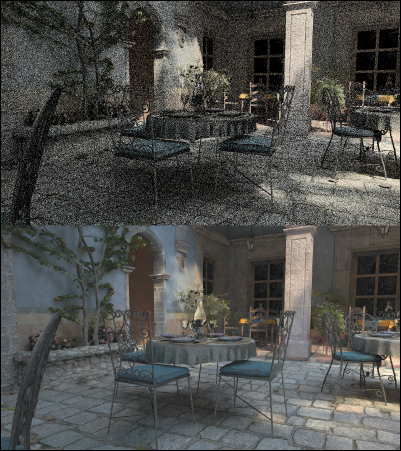
Figure 32.20: The eight samples per pixel that were used to generate the Monte Carlo rendering on top are filtered with RPF to produce the improved rendering on the bottom, which is virtually indistinguishable from a Monte Carlo rendering generated with 8,192 samples per pixel. (Courtesy of Pradeep Sen and Soheil Darabi, ©2012 ACM, Inc. Reprinted by permission.)
In this chapter, we’ve developed two renderers, but they are by no means state of the art. The book by Pharr and Humphreys [PH10] (which is nearly as large as this book) discusses physically based rendering in great detail, and is a fine choice for those who want to study rendering more deeply. The SIGGRAPH proceedings, other issues of the ACM Transactions on Graphics, and the proceedings of the Eurographics Symposium on Rendering give the student the opportunity to see how the ideas in this chapter originally developed, and which avenues of research proved to be dead ends and which have stood the test of time.
32.10. Exercises
Exercise 32.1: Up through Listing 32.10, we addressed the effects of the refractive index in two places in our program: in approximating the Fresnel term, and in computing the change in radiance at an interface between surfaces of different refractive indices. We did not, however, use the coefficient of extinction at all: Every material we considered transmits light perfectly, which means that all absorption takes place only at the boundaries between materials. Modify the path tracer to account for the coefficient of extinction of a material.
Exercise 32.2:(a) Let A = (0, 0), B = (1, 0), and C = (1, 1), and let T be the triangle ABC. Suppose that the texture coordinates for A are (uA, vA) = (0.2, 0.6), for B they’re (0.3, 0.3), and for C they’re (0.5, 0.1). Assume that texture coordinates are interpolated linearly across the triangle. Find the unit vector u such that the u-coordinate increases fastest in direction u.
(b) Generalize to arbitrary point and texture coordinates at the three vertices.
Exercise 32.3:(a) We used photon mapping to estimate the diffuse scattering of indirect light. Jensen suggests not even storing photons except on diffuse surfaces. And we also omit direct lighting from the photon mapping calculation—that gets handled in a separate step. But what would happen if you used photon mapping for specular reflections and direct lighting as well? What would you expect? Would a final gather be of any use?
(b) If you’ve written a photon-mapping renderer, try modifying it to handle each of these individually. Were your predictions correct?
Exercise 32.4:Our path tracer and photon mapper both assume that all light sources are “on the outside”—we don’t allow for a glowing lamp embedded in a glass sphere. Where in the code is the assumption embedded?
Exercise 32.5:(a) We merged the photon map with a ray tracer. Can you think of how to merge it with a path tracer instead?
(b) The photon mapper stops pushing around photons after some maximum depth; that introduces a bias. How? For a photon map that allows only n bounces, construct a scene where the resultant radiance estimate is drastically wrong, no matter how many photons you send into the scene.
(c) Can you take the idea from the path tracer—“just continue tracing until things stop”—and use it in the propagation of photons? Will it solve the problem with the scene you constructed in part (b)?
Exercise 32.6: (a) Given a random number generator that produces values uniformly in the interval [0, 1], describe how to generate uniform random points in the unit square.
(b) If you generate the point (x, y) with x < y, you can replace it with (y, x), and otherwise leave it unchanged. Show that this generates points uniformly in the triangle with vertices (0, 0), (1, 0), (1, 1).
(c) Let u = 1 – x, v = y, and w = 1 – (u+v). Show that applying this transformation to the results of part (b) generates points uniformly at random in barycentric coordinates on the triangle u + v + w = 1, 0 ≤ u, v, w, ≤ 1.
(d) Show that for any triangle PQR, the points uP + vQ + wR are distributed uniformly at random in the triangle, when uvw are generated according to part (c).
Exercise 32.7: (a) Write a WPF program that uses the method in Exercise 32.6 to generate points in a triangle. The user should be able to drag the three triangle vertices, and press buttons to generate either a single point or 100 points, each of which should be displayed as a colored dot within the triangle. Another button should clear the points.
(b) Extend your program to handle meshes. Generate a 2D mesh (perhaps the Delaunay triangulation for a random set of points), and then improve your program to pick a point (or 100 points) in the mesh uniformly at random. Do so by precomputing the triangle areas, summing them, and then assigning each triangle a probability given by its area divided by the total area. Put the triangles in some order, and compute probability sums s[0] = p[0], s[1] = p[0] + p[1], s[2] = p[0] + p[1] + p[2], etc. Given a uniform random variable u, you can now identify the largest index i with u ≤ s[i]. To generate a random mesh point, you can pick a uniform random number u, identify the last triangle i with u ≤ s[i], and then generate a random point in that triangle (see Exercise 32.6).
(c) Briefly discuss how to make the triangle-selection process faster than O(n), where n is the number of triangles in the mesh.
(d) Suppose that in ordering the triangles, we place the largest ones first. Then in a search of the list, we’re likely to examine relatively few triangles to find the “right” one. Would you, in working with a typical graphics model, expect this to have a large impact on the sampling time? Why or why not?
Exercise 32.8: We’ve argued that an eye ray hitting a point source is a probability-zero event, so we can ignore point sources. But since a point source is generally used to represent a limit of ever-tinier spherical sources, and for any such spherical source there’s a nonzero probability of an eye ray hitting it, the “can ignore” argument depends on what happens in these approximating cases. The radiance emitted by such a small approximating sphere is proportional to the inverse square of its radius (to maintain constant power); the probability of an eye ray hitting it is proportional to its squared radius; hence, the expected contribution to the pixel (once it’s small enough for its image to be completely contained in the pixel square on the film plane) is constant. We’re therefore treating the limit of a constant as zero. Adjust all the renderers in this chapter to make an extra pass to “correctly” render the effect of point lights by tracing a ray from each point light to the eye, and adding the appropriate radiance to the appropriate pixel if the point light’s actually visible. In doing this, you’re basically doing a special case of bidirectional path tracing.
Exercise 32.9: In the ray-trace-with-photon-mapping renderer, we estimate the direct light arriving from an area light with several samples. If the area light’s far away, this is probably overkill; if it’s nearby, it’s probably inadequate. For Lambertian reflectance of a uniformly emitting planar, one-sided area light, only the cosine term varies with the light-sample position. Suppose (see Figure 32.21) that the area light is completely contained in a sphere of radius s about some point Q, we’re reflecting it at a point P of some Lambertian surface, the “bright side” is completely visible from P, and the length of the vector r = Q – P from P to Q is d. Under what conditions on d and s can we approximate the reflected radiance due to the luminaire directly multiplying the projected area (orthogonal to r) of the source, the cosine of the angle θ between r and nP and the Lambertian reflectance, and 1 ||r||2 and be certain the result is correct within 1%? The several assumptions—that the source be planar, uniform, completely visible, etc., and that the reflecting surface be Lambertian—are not really as restrictive as they might sound. In particular, the same idea works for convex nonplanar sources, although the computation of the projected area may be nearly as complex as using multiple samples to estimate the reflected radiance.
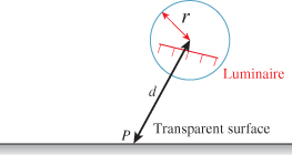
![]() (b) Suppose that the reflecting surface has a BRDF (for a fixed outgoing direction) whose variation, as a function of the incoming light direction θ, is nicely bounded, that is, |f (θ) – f (θ′)| < K|θ – θ′ |. Can you do an analogous analysis? See also Exercise 26.12 in Chapter 26.
(b) Suppose that the reflecting surface has a BRDF (for a fixed outgoing direction) whose variation, as a function of the incoming light direction θ, is nicely bounded, that is, |f (θ) – f (θ′)| < K|θ – θ′ |. Can you do an analogous analysis? See also Exercise 26.12 in Chapter 26.
Exercise 32.10: When we sampled points on an area light, we sampled uniformly with respect to area. We can instead presample a light source, using stratified sampling to generate a collection of samples that we can reuse. The stratified sampling helps ensure that the estimate of the average effect of the point light is accurate, although the estimates for adjacent pixels are likely to be highly correlated, which may be a problem in some cases. Essentially we’re replacing an area light with a collection of “micro-light” point lights. If there are too few, the shadows cast by each may generate a noticeable artifact.
(a) Build a ray tracer that replaces each area light with multiple point lights in this way. Do you see any artifacts? How is the running time affected as you increase the number of samples on the luminaire?
(b) Instead of using all the micro-lights to illuminate each surface point, we can pick one at random, essentially doing a single-sample estimate of the radiance transfer from the light to the surface point. Doing this once per primary ray can generate nice soft shadows. If we’re shooting 25 primary rays (using stratified sampling), and the area light is represented with 25 micro-lights, we’d like to use each micro-light once. How should you pair up the primary rays and the micro-lights? Do you foresee any problems?
(c) Implement your approach and critique the results.
Exercise 32.11: (a) Use the Poisson disk process to generate blue-noise samples on a line: Generate samples in the interval [0, 1] in which all are at least r = .001 apart, until there is no more room to fit a new sample.
(b) Discretize the interval into 10,000 bins, and record a 1 in each bin that contains a sample, and a 0 otherwise.
(c) Compute the fast Fourier transform of the resultant array. Does it appear to be a blue-noise distribution?
(d) Try this process again with various values for r. Below what frequency (in terms of r) is there relatively little energy?
(e) Now generate a similar occupancy array using stratified sampling, and compare the frequency spectra of the two processes. Describe any differences you find.
(f) Generalize to 2D.
(g) Implement Mitchell’s [Mit87] point diffusion algorithm for generating blue noise, and compare its results to the others.
Exercise 32.12: For a rectangular area light, write code to sample a point from the light uniformly with respect to area. Do the same for a spherical source. For the sphere, recall that the projection (x, y, z) ![]() (x/r, y, z/r), where
(x/r, y, z/r), where ![]() is an area-preserving map from the unit-radius cylinder about the y-axis, extending from y = –1 to y = 1, onto the unit sphere.
is an area-preserving map from the unit-radius cylinder about the y-axis, extending from y = –1 to y = 1, onto the unit sphere.