
Chapter 9. Functions on Meshes
9.1. Introduction
In mathematics, functions are often described by an algebraic expression, like f(x) = x2 + 1. Sometimes, on the other hand, they’re tabulated, that is, the values for each possible argument are listed, as in
A third, and very common, way to describe a function is to give its values at particular points and tell how to interpolate between these known values. For instance, we might plot the temperature at noon and midnight of each day of a week; such a plot consists of 15 distinct dots (see Figure 9.1). But we could also make a guess about the temperatures at times between each of these, saying, for instance, that if it was 60° at noon and 24° at midnight, that drop of 36° took place at a steady rate of 3° per hour. In other words, we would be linearly interpolating to define the function for all times rather than just at noon and midnight each day. The resultant function, defined on the whole week rather than just the 15 special times, is a connect-the-dots version of the original.
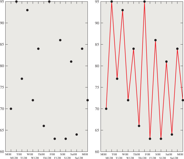
Figure 9.1: The temperature at noon and midnight for each day in a week. The domain of this function consists of 15 points. When we linearly interpolate the values between pairs of adjacent points, we get a function defined on the whole week—a connect-the-dots version of the original.
Let’s now write that out in equations. Suppose that t0 < t1 < t2 < ... < tn are the times at which the temperature is known, and that f0, f1, ..., fn are the temperatures in degrees Fahrenheit at those times.
Then
where
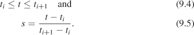
Further suppose that the times are measured in 12-hour units, starting at midnight Sunday, so t0 = 0, t1 = 1, etc.
In this formulation i is the index of the interval containing t, and s describes the fraction of the way from ti to ti+1 where t lies (when t = ti, s is zero; when t = ti+1, s is one).
Suppose that t0 = 0, t1 = 1, etc., and that f0 = 7, f1 = 3, and f2 = 4; evaluate f(1. 2) by hand. If we changed f0 to 9, would it change the value you computed? Why or why not?
Just as we can have barycentric coordinates on a triangle (see Section 7.9.1), we can place them on an interval [p, q] as well. The first coordinate varies from one at p to zero at q; the second varies from zero at p to one at q. Their sum is everywhere one that is, for every point of the interval [p, q], the sum is one (see Exercise 9.8). With these barycentric coordinates, we can write a slightly more symmetric version of the formula above:
where c0(t) is the first barycentric coordinate of t and c1(t) is the other.
This “continuous extension” of f has analogs for other situations. Before we look at those, let’s examine some of the properties. First, the value of the interpolated function at noon or midnight each day (ti) is just fi; it doesn’t depend at all on the values at noon or midnight on the other days. Second, the value at noon on one day influences the shape of the graph only for the 12 hours before and the 12 hours after. Third, the interpolated function is in fact continuous.
Now let’s consider interpolating values given at discrete points on a surface. Since we often use triangle meshes in graphics to represent surfaces, let’s suppose that we have a function whose values are known at the vertices of the mesh; the value at vertex i is fi. How can we “fill in” values at the other points of all the triangles in the mesh?
By analogy, we use barycentric coordinates. Consider a point P in a triangle with vertices v0, v1, and v2 (see Figure 9.2); we can define
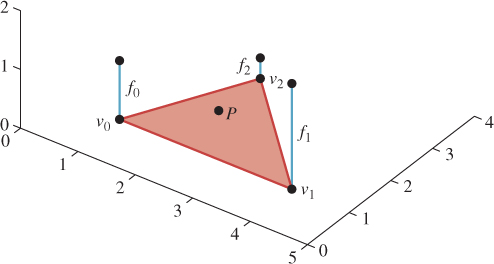
Figure 9.2: The point P is in the triangle with vertices v0, v1, and v2, where the function has values f0, f1, and f2, respectively. What value should we assign to the point P?
where (c0, c1, c2) are the barycentric coordinates of P with respect to v0, v1, and v2.
Once again, the interpolated function has several nice properties. First, the value at the vertex vi is just fi; the value along the edge from vi to vj (assuming they are adjacent) depends only on fi and fj; thus, for a point q on such an edge, it doesn’t matter which of the two triangles sharing the edge from vi to vj is used to compute f(q)—the answer will be the same! Second, the value fi at vertex vi again influences other values only locally, that is, only on triangles that contain the vertex vi. Third, the interpolated function is in fact continuous.
The remainder of this chapter investigates this idea of interpolating across faces, its relationship to barycentric coordinates, and some applications.
9.2. Code for Barycentric Interpolation
The discussion so far has been somewhat abstract; we’ll now write some code to implement these ideas. Let’s start with a simple task.
Input:
• A triangle mesh in the form of an n × 3 table, vtable, of vertices
• A k × 3 table, ftable, of triangular faces, where each row of ftable contains three indices into vtable
• An n × 1 table, fntable, of function values at the vertices of the mesh
• A point P of the mesh, expressed by giving the index, t, of the triangle in which the point lies, and its barycentric coordinates α, β, γ in that triangle
Output:
• The value of the interpolated function at P
The first thing to realize is that only the tth row of ftable is relevant to our problem: The point P lies in the tth triangle; the other triangles might as well not exist. If the tth triangle has vertex indices i0, i1, and i2, then only those entries in vtable matter. With this in mind, our code is quite simple:
1 double meshinterp(double[,] vtable, int[,] ftable,
2 double[] fntable, int t, double alpha, double beta, double gamma)
3 {
4 int i0 = ftable[t, 0];
5 int i1 = ftable[t, 1];
6 int i2 = ftable[t, 2];
7 double fn0 = fntable[i0];
8 double fn1 = fntable[i1];
9 double fn2 = fntable[i2];
10 return alpha*fn0 + beta*fn1 + gamma*fn2;
11 }
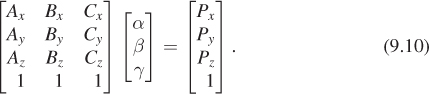
Now suppose that P is given differently: We are given the coordinates of P in 3-space rather than the barycentric coordinates, and we are given the index t of the triangle to which P belongs, and we need to find the barycentric coordinates α, β, and γ. If we say that the vertices of the triangle t are A, B, and C, we want to have
where the subscript x indicates the first coordinate of a point; we must also satisfy the same equations for y and z. But there’s one more equation that has to hold: α + β + γ = 1. We can rewrite that in a form that’s analogous to the others:
Now our system of equations becomes
There’s really no solution here except to directly solve the system of equations. The problem is that we have four equations in three unknowns, and most solvers want to work with square matrices rather than rectangular ones. (Section 7.9.2 presented an alternative approach to this problem using some precomputation, but that precomputation amounts to doing much of the work of solving the system of equations.)
The good news is that the four equations are in fact redundant: The fact that P is given to us as a point of the triangle ensures that if we simply solve the first three equations, the fourth will hold. That assurance, however, is purely mathematical—computationally, it may happen that small errors creep in. There are several viable approaches.
• Express P as a convex combination of four points of R4: the three already written and a fourth, with coordinates nx, ny, nz, and 0, where n is the normal vector to the triangle. The expression will have a fourth coefficient, δ, in the solution, representing the degree to which P is not in the plane of A, B, and C. We ignore this and scale up the computed α, β, and γ accordingly, using α/(1 – δ), β/(1 – δ), and γ/(1 – δ) as the barycentric coordinates. This is a good solution (in the sense that if the numerical error in P is entirely in the n direction, the method produces the correct result), but it requires solving a 4 × 4 system of equations.
• Delete the fourth row of the system in Equation 9.10; adjust α, β, and γ to sum to one by dividing each by α + β + γ. This reduces the problem to a 3×3 system, but it lacks the promise of correctness for normal-only errors.
• Use the pseudoinverse to solve the overconstrained system (see Section 10.3.9). This has the advantage that it’s already part of many numerical linear algebra systems, and that it works even when the triangle is degenerate (i.e., the three points are collinear), in the sense that if P lies in the triangle, then the method produces numbers α, β, and γ with αA + βB + γC = P, even though the solution in this case is not unique. Better still, if P is not in the plane of A, B, and C, the solution returned will have the property that αA + βB + γC is the point in the plane of A, B, and C that’s closest to P. This is therefore the ideal.
So the restated problem looks like this.
Input:
• A triangle mesh in the form of an n × 3 table, vtable, of vertices
• A k × 3 table, ftable, of triangles, where each row of ftable contains three indices into vtable
• A point P of the mesh, expressed by giving the index, t, of the triangle in which the point lies, and its coordinates in 3-space
Output:
• The value of the barycentric coordinates of P with respect to the vertices of the kth triangle
And our revised solution is this:
1 double[3] barycentricCoordinates(double[,] vtable,
2 int[,] ftable, int t, double p[3])
3 {
4 int i0 = ftable[t, 0];
5 int i1 = ftable[t, 1];
6 int i2 = ftable[t, 2];
7 double[,] m = new double[4, 3];
8 for (int j = 0; j < 3; j++) {
9 for (int i = 0; i < 3; i++) {
10 m[i,j] = vtable[ftable[t, j], i];
11 }
12 m[3,j] = 1;
13 }
14
15 k = pseudoInverse(m);
16 return matrixVectorProduct(k, p);
17 }
Here we’ve assumed the existence of a matrix-vector product procedure and a pseudoinverse procedure, as provided by most numerical packages.
The two procedures above can be combined, of course, to produce the function value at a point P that’s specified in xyz-coordinates.
Input:
• A triangle mesh in the form of an n × 3 table, vtable, of vertices
• A k × 3 table, ftable, of triangles, where each row of ftable contains three indices into vtable
• An n × 1 table, fntable, of function values at the vertices of the mesh
• A point P of the mesh, expressed by giving the index, t, of the triangle in which the point lies, and its coordinates in 3-space
Output:
• The value of the function defined by the function table at the point P
1 double meshinterp2(double[,] vtable, int[,] ftable, double[] fntable,
2 int t, double p[3])
3 {
4 double[] barycentricCoords =
5 barycentricCoordinates(vtable, ftable, t, p);
6 return meshinterp(vtable, ftable, fntable, t,
7 barycentricCoords[0], barycentricCoords[1], barycentricCoords[2]);
8 }
Of course, the same idea can be applied to the ray-intersect-triangle code of Section 7.9.2, where we first computed the barycentric coordinates (α, β, γ) of the ray-triangle intersection point Q with respect to the triangle ABC, and then computed the point Q itself as the barycentric weighted average of A, B, and C. If instead we had function values fA, fB, and fC at those points, we could have computed the value at Q as fQ = αfA + βfB + γfC. Notice that this means we can compute the interpolated function value fQ at the intersection point without ever computing the intersection point itself!
Computing barycentric coordinates (α, β, γ) for a point P of a triangle ABC, where A, B, C ε R2, is somewhat simpler than the corresponding problem in 3-space (see Figure 9.3). We know that the lines of constant α are parallel to BC. If we let n = (C – B)⊥, then the function defined by f(P) = (P – B) · n is also constant on lines parallel to B – C. Scaling this down by f(A) gives us the function we need: It’s zero on line BC, and it’s one at A. So we let
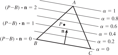
Figure 9.3: To write the point P as αA + βB + γC, we can use a trick. For points on line BC, we know α = 0; on any line parallel to BC, α is also constant. We can compute the projection of P – B onto the vector n that’s perpendicular to BC; this also gives a linear function that’s constant on lines parallel to BC. If we scale this function so that its value at A is 1, we must have the function α.
and the value of g(P) is just α. A similar computation works for β and γ.
The resultant code looks like this:
1 double[3] barycenter2D(Point P, Point A, Point B, Point C)
2 C[2])
3 {
4 double[] result = new double[3];
5 result[0] = helper(P, A, B, C);
6 result[1] = helper(P, B, C, A);
7 result[2] = helper(P, C, A, B);
8 return result;
9 double helper(Point P, Point A, Point B, Point C)
10 {
11 Vector n = C - B;
12 double t = n.X;
13 n.X = -n.Y; // rotate C-B counterclockwise 90 degrees
14 n.Y = t;
15 return dot(P - B, n) / dot(A - B, n);
16 }
Of course, if the triangle is degenerate (e.g., if A lies on line BC), then the dot product in the denominator of the helper procedure will be zero; then again, in this situation the barycentric coordinates are not well defined. In production code, one needs to check for such cases; it would be typical, in such a case, to express P as a convex combination of two of the three vertices.
9.2.1. A Different View of Linear Interpolation
One way to understand the interpolated function is to realize that the interpolation process is linear. Suppose we have two sets of values, {fi} and {gi}, associated to the vertices, and we interpolate them with functions F and G on the whole mesh. If we now try to interpolate the values {fi + gi}, the resultant function will equal F + G. That is to say, we can regard barycentric interpolation on the mesh as a function from “sets of vertex values” to “continuous functions on the mesh.” Supposing there are n vertices, this gives a function
where C(M) is the set of all continuous functions on the mesh M. What we’ve just said is that
where f denotes the set of values {f1, f2, ..., fn}, and similarly for g; the other linearity rule—that I(αf) = αI(f) for any real number α—also holds.
A good way to understand a linear function is to examine what it does to a basis. The standard basis for Rn consists of elements that are all zero except for a single entry that’s one. Each such basis vector corresponds to interpolating a function that’s zero at all vertices except one—say, v—and is one at v (see Figure 9.4).
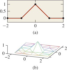
Figure 9.4: (a) The 2D interpolating basis function is tent-shaped near its center; (b) in 3D, for a mesh in the xy-plane, we can graph the function in z and again see a tentlike graph that drops off to zero by the time we reach any triangle that does not contain v.
The resultant interpolant is a basis function that has a graph that looks tentlike, with the peak of the tent sitting above the vertex where the value is one.
If we add up all these basis functions, the result is the function that interpolates the values 1, 1, ..., 1 at all the vertices; this turns out to be the constant function 1. Why? Because the barycentric coordinates of every point in every triangle sum to one.
One might look at these tent-shaped functions and complain that they’re not very continuous in the sense that they are continuous but not differentiable. Wouldn’t it be nicer to use basis functions that looked like the ones in Figure 9.5? It would, but it turns out to be more difficult to have both the smoothness property and the property that the interpolant for the “all ones” set of values is the constant function 1. We’ll discuss this further in Chapter 22.

Figure 9.5: Basis functions for (a) 2D and (b) 3D interpolations that are smoother than the barycentric-interpolation functions.
9.2.1.1. Terminology for Meshes
This section introduces a few terms that are useful in discussing meshes. First, the vertices, edges, and faces of a mesh are all called simplices. Simplices come in categories: A vertex is a 0-simplex, an edge is a 1-simplex, and a face is a 2-simplex. Simplices contain their boundaries, so a 2-simplex in a mesh contains its three edges and a 1-simplex contains its two endpoints.
The star of a vertex (see Figure 9.6) is the set of triangles that contain that vertex. More generally, the star of a simplex is the set of all simplices that contain it.
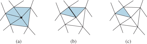
Figure 9.6: The star of a simplex. (a) The star of a vertex is the set of triangles containing it, (b) the star of an edge is the two triangles containing it, and (c) the star of a triangle is the triangle itself.
The boundary of the star of a vertex is called the link of the vertex. This is useful in describing functions like the tent functions above: We can say that the tent has value 1 at the vertex v, has nonzero values only on the star of v, and is zero on the link of v.
There’s a notion of “distance” in a mesh based on edge paths between vertices: The distance from v to w is the smallest number of edges in any chain of edges from v to w. Thus, all the vertices in the link of v have a mesh distance of one from v.
The sets of vertices at various distances from v have names as well. The 1-ring is the set of vertices whose distance from v is one or less; the 2-ring is the set of vertices whose distance from v is two or less, etc.
9.2.2. Scanline Interpolation
Frequently in graphics we need to compute some value at each point of a triangle; for example, we often compute an RGB color triple at each vertex of a triangle, and then interpolate the results over the interior (perhaps because doing the computation that produced the RGB triple at the vertices would be prohibitive if carried out for every interior point).
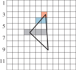
In the 1980s, when raster graphics (pixel-based graphics) technology was new, scanline rendering was popular. In scanline rendering, each horizontal line of the screen was treated individually, and all the triangles that met a line were processed to produce a row of pixel values, after which the renderer moved on to the next line. Usually the new scanline intersected many of the same triangles as the previous one, and so lots of data reuse was possible. Figure 9.7 shows a typical situation: At row 3, only the orange pixel meets the triangle; at row 4, the two blue pixels do. At row 6, the four gray pixels meet the triangle, and after that the intersecting span begins to shrink.
One scheme that was used for interpolating RGB triples was to interpolate the vertex values along each edge of the triangle, and then to interpolate these across each scanline.
It’s not difficult to show that this results in the same interpolant as the barycentric method we described (see Exercise 9.4).
But now suppose that we apply this method to a more interesting shape, like a quadrilateral. It’s easy to see that the two congruent squares in Figure 9.8, with gray values of 0, 40, 0, and 40 (in a range of 0 to 40) assigned to their vertices in clockwise order, lead to different interpolated values for the points P and P′, the first being 20 and the second being 40.
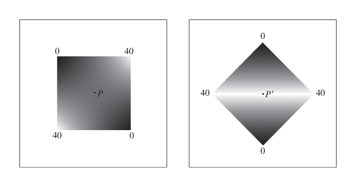
Figure 9.8: The congruent squares in these two renderings have the same gray values at corresponding vertices, but the scanline-interpolated gray values at P and P′ differ.
The interpolated values in each configuration look decent, but when one makes an animation by rotating a shape, the interior coloring or shading seems to “swim” in a way that’s very distracting.
What went wrong?
The problem was to infer values at the interior points of a polygon, given values at the vertices. But the solution depends on something unrelated to the problem, namely the scanlines in the output; this dependence shows up as an artifact in the results. The difficulty is that the solution is not based on the mathematics and physics of the problem, but rather on the computational constraints on the solution. When you limit the class of solutions that you’re willing to examine a priori, there’s always a chance that the best solution will be excluded. Of course, sometimes there’s a good reason to constrain the allowable solutions, but in doing so, you should be aware of the consequences. We embody these ideas in a principle:
![]() The Division of Modeling Principle
The Division of Modeling Principle
Separate the mathematical and/or physical model of a phenomenon from the numerical model used to represent it.
Attempting to computationally solve a problem often involves three separate choices. The first is an understanding of the problem; the second is a choice of mathematical tools; the third is a choice of computational method. For example, in trying to model ocean waves, we have to first look at what’s known about them. There are large rolling waves and there are waves that crest and break. The first step is to decide which of these we want to simulate. Suppose we choose to simulate rolling (nonbreaking) waves. Then we can represent the surface of the water with a function, y = f(t, x, z), expressing the height of the water at the point (x, z) at time t. Books on oceanography give differential equations describing how f changes over time. When it comes to solving the differential equation, there are many possible approaches. Finite-element methods, finite-difference methods, spectral methods, and many others can be used. If we choose, for example, to represent f as a sum of products of sines and cosines of x and z, then solving the differential equations becomes a process of solving systems of equations in the coefficients in the sums. If we limit our attention to a finite number of terms, then this problem becomes tractable.
But having made this choice, we can see certain influences: Because there’s a highest-frequency sine or cosine in our sum, there’s a smallest possible wavelength that can be represented. If we want our model to contain ripples smaller than this, the numerical choice prevents it. And if, having solved the problem, we decide we’d like to make waves that actually crest and break, our mathematical choice precludes it. We can, of course, add a “breaking wave” adjustment to the output of our model, altering the shapes of certain wave crests, but it should come as no surprise that such an ad hoc addition is more likely to produce problems than good results. Furthermore, it will make debugging of our system almost impossible, because without a clear notion of the “right solution,” it’s very difficult to detect an error conclusively.
The idea of carefully structuring your models and separating the mathematical from the numerical is discussed at length by Barzel [Bar92].
9.3. Limitations of Piecewise Linear Extension
The method of extending a function on a triangle mesh from vertices to the interiors of triangles is called piecewise linear extension. By looking at the basis functions—the tent-shaped graphs—we can see that the graphs of such extensions will have sharp corners and edges. Depending on the application, these artifacts may be significant. For instance, if we interpolate gray values across a triangle mesh, the human eye tends to notice the second-order discontinuities at triangle edges: When the gray values change linearly across the triangle interiors, things look fine; when the rate of change changes at a triangle edge, the eye picks it out.
Some people tend to see “bands” near such discontinuities; the effect is called Mach banding (see Section 1.7).
If we use piecewise linear interpolation in animation, having computed the positions of objects at certain “key” times, then between these times objects move with constant velocities, and hence zero acceleration; all the acceleration is concentrated in the key moments. This can be very distracting.
9.3.1. Dependence on Mesh Structure
If we have a polyhedral shape with nontriangular faces, we can triangulate each face to get a triangle mesh. Then we can, as before, interpolate function values at the vertices over the triangular faces. But the results of this interpolation can vary wildly depending on the particular triangulation. It’s easiest to see this with a very simple example (see Figure 9.9) in which a function defined on the corners of a square is extended to the interior in two different ways. The results are evidently triangulation-dependent.
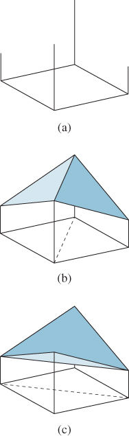
Figure 9.9: (a) A square with heights assigned at the four corners; (b) one piecewise linear interpolation of these values; and (c) a different interpolation of the same values.
9.4. Smoother Extensions
As we hinted above, taking function values at the vertices of a mesh and trying to find smoothly interpolated values over the interior of the mesh is a difficult task. Part of the difficulty arises in defining what it means to be a smooth function on a mesh. If the mesh happens to lie in the xy-plane, it’s easy enough: We can use the ordinary definition of smoothness (existence of various derivatives) on the plane. But when the mesh is simply a polyhedral surface in 3-space (e.g., like a dodecahedron), it’s no longer clear how to measure smoothness.
Of course, if we replace the dodecahedron with the sphere that passes through its vertices, then defining smoothness is once again relatively easy. Each point of the dodecahedron corresponds to a point on the surrounding sphere (e.g., by radial projection), and we can declare a function that’s smooth on the sphere to be smooth on the dodecahedron as well. Unfortunately, finding a smooth shape that passes through the vertices of a polyhedron is itself an instance of the extension problem: We have a function (the xyz-coordinates of a point) defined at each vertex of the mesh; we’d like a function (the xyz-coordinates of the smooth-surface points) that’s defined on the interiors of triangles. Such a function is what a solution to the smooth interpolation problem would give us. Thus, in suggesting that we use a smooth approximating shape, we haven’t really simplified the problem at all.
A partial solution to this is provided by creating a sequence of meshes through a process called subdivision of the original surface. These subdivided meshes converge, in the limit, to a fairly smooth surface. We’ll discuss this further in Chapter 22.
9.4.1. Nonconvex Spaces
The piecewise linear extension technique works when the values at the vertices are real numbers; it’s easy to extend this to tuples of real numbers (just do the extension on one coordinate at a time). It’s also easy to apply it to other spaces in which convex combinations, that is,
make sense. For example, if you have a 2 × 2 symmetric matrix associated to each vertex, you can perform barycentric blending of the matrices, because a convex combination of symmetric matrices is still a symmetric matrix.
Unfortunately, there are many interesting spaces in which convex combinations either don’t make sense or fail to be defined for certain cases. The exemplar is the circle S1. If you treat the circle as a subset of R2, then (see Figure 9.10) forming convex combinations of two points makes sense . . . but the result is a point in the unit disk D2 ![]() R2, and generally not a point on S1.
R2, and generally not a point on S1.
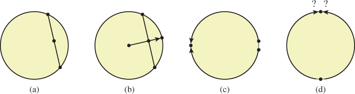
Figure 9.10: (a) If we take convex combinations of points on a circle in R2, the result is a point in R2, but it is not generally on the circle; (b) if we radially project back to the circle, it works better . . . but the value is undefined when the original convex combination falls at the origin. (c) If we do angular interpolation, the point halfway between 355° and 5° turns out to be 180°. (d) If we try angular interpolation along the shortest route, our blend becomes undefined when the points are opposites.
The usual attempt at solving this is to “re-project” back to the circle, replacing the convex combination point C with C/||C||. Unfortunately, this fails when C turns out to be the origin. The problem is not one that can be solved by any clever programming trick.
![]() It’s a fairly deep theorem of topology that if
It’s a fairly deep theorem of topology that if
has the property that h(p) = p for all points of S1, then h must be discontinuous somewhere.
Another possible approach is to treat the values as angles, and just interpolate them. Doing this directly leads to some oddities, though: Blending some points in S1 that are very close (like 350° and 10°) yields a point (180° in this case) that’s far from both. Doing so by “interpolating along the shorter arc” addresses that problem, but it introduces a new one: There are two shortest arcs between opposite points on the circle, so the answer is not well defined.
![]() Once again, a theorem from topology explains the problem. If we simply consider the problem of finding a halfway point between two others, then we’re seeking a function
Once again, a theorem from topology explains the problem. If we simply consider the problem of finding a halfway point between two others, then we’re seeking a function
with certain properties. For instance, we want H to be continuous, and we want H(p, p) = p for every point p ![]() S1, and we want H(p, q) = H(q, p), because “the halfway point between p and q” should be the same as “the halfway point between q and p.” It turns out that even these two simple conditions are too much: No such function exists.
S1, and we want H(p, q) = H(q, p), because “the halfway point between p and q” should be the same as “the halfway point between q and p.” It turns out that even these two simple conditions are too much: No such function exists.
![]() The situation is even worse, however: Interpolation between pairs of points, if it were possible, would let us extend our function’s domain from vertices to edges of the mesh. Suppose that somehow we were given such an extension; could we then extend continuously over triangles? Alas, no. The study of when such extensions exist is a part of homotopy theory, and particularly of obstruction theory [MS74]. We mention this not because we expect you to learn obstruction theory, but because we hope that the existence of theorems like the ones above will dissuade you from trying to find ad hoc methods for extending functions whose codomains don’t have simple enough topology.
The situation is even worse, however: Interpolation between pairs of points, if it were possible, would let us extend our function’s domain from vertices to edges of the mesh. Suppose that somehow we were given such an extension; could we then extend continuously over triangles? Alas, no. The study of when such extensions exist is a part of homotopy theory, and particularly of obstruction theory [MS74]. We mention this not because we expect you to learn obstruction theory, but because we hope that the existence of theorems like the ones above will dissuade you from trying to find ad hoc methods for extending functions whose codomains don’t have simple enough topology.
9.4.2. Which Interpolation Method Should I Really Use?
The problem of interpolating over the interior of a triangle applies in many situations. If we are interpolating a color value, then linear interpolation in some space where equal color differences correspond to equal representation distances (see Chapter 28) makes sense. If we are interpolating a unit normal vector value, then linear interpolation is surely wrong, because the interpolated normal will generally not end up a unit vector, and if you use it in a computation that relies on unit normals, you’ll get the wrong answer. And if the value is something discrete, like an object identifier, then interpolation makes no sense at all.
All of this seems to lead to the answer, “It depends!” That’s true, but there’s something deeper here:
![]() The Meaning Principle
The Meaning Principle
For every number that appears in a graphics program, you need to know the semantics, the meaning, of that number.
Sometimes this meaning is given by units (“That number represents speed in meters per second”); sometimes it helps you place a bound on possible values for a variable (“This is a solid angle,1 so it should be between 0 and 4π ≈ 12.5” or “This is a unit normal vector, so its length should be 1.0”); and sometimes the meaning is discrete (“This represents the number of paths that have ended at this pixel”). It’s important to distinguish the meaning of the number from its representation. For instance, we often are interested in the coverage of a pixel (how much of a small square is covered by some shape) as a number α between zero and one, but α is sometimes represented as an 8-bit unsigned integer, that is, an integer between 0 and 255. Despite the discrete nature of the representation, it makes perfectly good sense to average two coverage values (although representing the average in the 8-bit form may introduce a roundoff error, of course).
1. Solid angles are discussed in Chapter 26.
9.5. Functions Multiply Defined at Vertices
Until now, we’ve discussed the very common case of functions that have a single value at each vertex and need to be interpolated across faces. But another situation arises frequently in graphics: a function where there’s a value at each vertex for each triangle that meets that vertex. Consider, for instance, the colored octahedron in Figure 9.11. Each triangle has a color gradient across it, but no two triangles have the same color at each vertex. The way to generate a color function for this shape is to consider a function defined on a larger domain than the vertices. Consider all vertex-triangle pairs in which the triangle contains the vertex, that is,
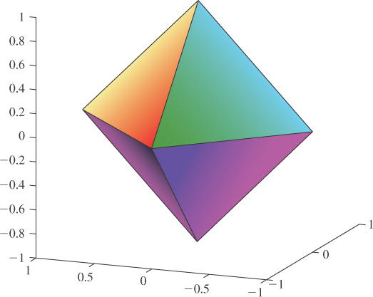
Figure 9.11: An octahedron on which each face has a different color gradient. At each vertex of the octahedron, we need to store four different colors, one for each of the faces.
where V and T are the sets of vertices and triangles of the mesh, respectively. Until now, we’ve taken a function defined h in V and extended it to all points of the mesh. We now instead define a function on Q and extend this to all points of the mesh. A point in a triangle t with vertices i, j, and k gets its value by a barycentric interpolation of the values h(i, t), h(j, t), and h(k, t).
This leads to one important problem: A point on the edge (i, j) is a point of two different triangles. What color should it have? The answer is “It depends.” From a strictly mathematical standpoint, there’s no single correct answer; there will be a color associated to the interpolation of colors on one face, and a different one associated to the interpolation of colors on the other face. Neither is implicitly “right.” The best we can do is to say that interpolation defines a function on
where P is a point of the mesh M; that is, for each point P and each triangle t that contains it, we get a value h(P, t). Since most points are in only one triangle, the second argument is generally redundant. But for those in more than one triangle, the function value is defined only with reference to the triangle under consideration.
9.6. Application: Texture Mapping
We mentioned in Chapter 1 that models are often described not only by geometry, but by textures as well: To each point of an object, we can associate some property (surface color is a common one), and this property is then used in rendering the object. At a high level, when we are determining the color of a pixel in a rendering we typically base that computation on information about the underlying object that appears at that pixel; if it’s a triangle of some mesh, we use, for instance, the orientation of that triangle in determining how brightly lit the point is by whatever illumination is in the scene. In some cases, the triangle may have been assigned a single color (i.e., its appearance under illumination by white light), which we also use, but in others there may be a color associated to each vertex, as in the previous section, and we can interpolate to get a color at the point of interest. Very often, however, the vertices of the triangle are associated to locations in a texture map, which is typically some n × k image; it’s easy to think of the triangle as having been stretched and deformed to sit in the image. The color of the point of interest is then determined by looking at its location in the texture map, as in Figure 9.12, and finding the color there.
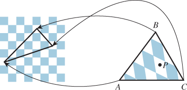
Figure 9.12: The point P of the triangle T = ΔABC has its color determined by a texture map. The points A, B, and C have been assigned to points in the checkerboard image, as shown by the arrows; the point P corresponds to a point in a white square, so its texture color is white.
9.6.1. Assignment of Texture Coordinates
When we say that sometimes the vertices of the triangle are associated to locations in a texture map, it’s natural to ask, “How did they get associated?” The answer is “by the person who created the model.” There are some simple models for which the association is particularly easy. If we start with an n × k grid of triangles as shown in Figure 9.13, top, with n = 6 and k = 8, we can associate to each vertex (i, j) of this mesh a point in 3-space by setting
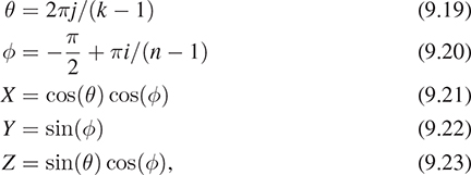
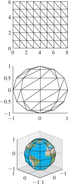
that is, letting θ and φ denote longitude and latitude, respectively. The approximately spherical shape that results is shown in the middle. We also have a 100 × 200 texture image of an “unprojected” map of the Earth (the vertical coordinate is proportional to latitude; the horizontal proportional to longitude). We assign texture coordinates 100i/(n – 1), 200j/(k – 1) to the vertex at position (i, j), and the resultant globe is shown rendered with the texture map at the bottom.
In this case, the way we created the mesh made it natural to create the texture coordinates at the same time. There is one troubling aspect of this approach, though: The texture coordinates depend on the number of pixels in the image that we use as our world map. If we created this shape and decided that the result looked bad, we might want to use a higher-resolution image, but that would entail changing the texture coordinates as well. Because of this, texture coordinates are usually specified as numbers between zero and one, representing a fraction of the way up2 or across the image, so texture coordinates (0.75, 0.5) correspond to a point three-quarters of the way up the texture image (regardless of size) and midway across, left to right.
2. Or down, if the image pixels are indexed from top to bottom, as often happens.
It’s commonplace to name these texture coordinates u and v so that a typical vertex now has five attributes: x, y, z, u, and v. Sometimes texture coordinates are referred to as uv-coordinates.
9.6.2. Details of Texture Mapping
If we have a mesh with texture coordinates assigned at each vertex, how do we determine the texture coordinates at some location within a triangle? We use the techniques of this chapter, one coordinate at a time. For instance, we have a u-coordinate at every vertex; such an assignment of a real value at every vertex uniquely defines a piecewise linear function at every point of the mesh: If P is a point of the triangle ABC, and the u-coordinates of A, B, and C are uA, uB, and uC, we can determine a u-coordinate for P using barycentric coordinates. We write P in the form
and then define
We can do the same thing for v, and this uniquely determines the uv-coordinates for P.
If the triangle ABC happens to cover many pixels, we’ll do this computation—find the barycentric coordinates and use them to combine the texture coordinates from the vertices—many times. Fortunately, the regularity of pixel spacing makes this repeated computation particularly easy to do in hardware, as described in Chapter 38.
9.6.3. Texture-Mapping Problems
If a triangle has texture coordinates that make it cover a large area of the texture image, but the triangle itself, when rendered, occupies a relatively small portion of the final image, then each pixel in the final image (thought of as a little square) corresponds to many pixels in the texture image. Our approach finds a single point in the texture image for each final image pixel, but perhaps it seems that the right thing to do would be to blend together many texture image pixels to get a combined result. If we do not do this, we get an effect called texture aliasing, which we’ll discuss further in Chapters 17, 20 and 38. If we do blend together texture image pixels for each pixel to be rendered, the texturing process becomes very slow. One way to address this is through precomputation; we’ll discuss a particular form of this precomputation, called MIP mapping, in Chapter 20.
9.7. Discussion
The main idea of this chapter is so simple that many graphics researchers tend to not even notice it: A real-valued function on the vertices of a mesh can be extended piecewise linearly to a real-valued function on the whole mesh, via the barycentric coordinates on each triangle. In a triangle with vertices vi, vj, and vk, where the values are fi, fj, and fk, the value at the point whose barycentric coordinates are ci, cj, and ck is cifi + cjfj + ckfk. This extension from vertices to interior is so ingrained that it’s done without mention in countless graphics papers. There are other possible extensions from values at vertices to values on whole triangles, some of which are discussed in Chapter 22, but this piecewise linear interpolation dominates.
This same piecewise linear interpolation method works for functions with other codomains (e.g., R2 or R3), as long as those codomains support the idea of a “convex combination.” For domains that do not (like the circle, or the sphere, or the set of 3 × 3 rotation matrices) there may be no reasonable way to extend the function over triangles.
Solving problems like this interpolation from vertices in the abstract helps avoid implementation-dependent artifacts. If we had studied the problem in the context of interpolating values represented by 8-bit integers across the interior of a triangle in a GPU, we might have gotten distracted by the low bit-count representation, rather than trying to understand the general problem and then adapt the solution to our particular constraints. This is another instance of the Approximate the Solution principle.
One important application of piecewise linear interpolation is texture mapping, in which a property of a surface is associated to each vertex, and these property values are linearly interpolated over the interiors of triangles. If the property is “a location in a texture image,” then the interpolated values can be used to add finely detailed variations in color to the object. Chapter 20 discusses this.
9.8. Exercises
![]() Exercise 9.1: The basis functions we described in this chapter, shown in Figure 9.4(a), not only correspond to a basis for Rn, they also form a basis of another vector space—a subspace of the vector space of all continuous functions on the domain [1, n]. To justify this claim, show that these functions are in fact linearly independent as functions.
Exercise 9.1: The basis functions we described in this chapter, shown in Figure 9.4(a), not only correspond to a basis for Rn, they also form a basis of another vector space—a subspace of the vector space of all continuous functions on the domain [1, n]. To justify this claim, show that these functions are in fact linearly independent as functions.
Exercise 9.2: (a) Draw a tetrahedron; pick a vertex and draw its link and its star. Suppose v and w are distinct vertices of the tetrahedron. What is the intersection of the star of v and the star of w?
(b) Draw an octahedron, and answer the same question when v is the top vertex and w is the bottom one.
Exercise 9.3: Think about a manifold mesh that contains vertices, edges, triangles, and tetrahedra. You could call this a solid mesh rather than a surface mesh. Consider a nonboundary vertex of such a mesh. What is the topology of the star of the vertex? What is the topology of the link of the vertex?
Exercise 9.4: Show that the interpolation of values across a triangle using the scanline method is the same as the one defined using the barycentric method. Hint: Show that if the triangle is in the xy-plane, then each of the methods defines a function of the form f(x, y) = Ax + By + C. Now suppose you have two such functions with the same values at the three vertices of a triangle. Explain why they must take the same values at all interior points as well.
![]() Exercise 9.5: The function H of Equation 9.16 cannot exist; here’s a reason why. Suppose that it did. Define a new function
Exercise 9.5: The function H of Equation 9.16 cannot exist; here’s a reason why. Suppose that it did. Define a new function
where we’re implicitly using the correspondence of the number θ in the interval [0, 2π] with the point (cos θ, sin θ) of S1. Now consider the loop in the domain of K consisting of three straight lines, from (0, 0) to (2π, 0), from (2π, 0) to (2π, 2π), and from (2π, 2π) back to (0, 0).
(a) Draw this path.
(b) For each point p of this path, K(p) is an element of S1. Restricting K to this path gives a map from the path to S1 ![]() R2. We can compute the winding number of this path about the origin in R2. Explain, using the assumed properties of H, why the winding numbers of the first two parts of the path must be equal.
R2. We can compute the winding number of this path about the origin in R2. Explain, using the assumed properties of H, why the winding numbers of the first two parts of the path must be equal.
(c) Explain why the winding number of the last part must be one.
(d) Conclude that the total winding number must be odd.
(e) Now consider shrinking the triangular loop toward the center of the triangle. The winding number will be a continuous integer-valued function of the triangle size. Explain why this means the winding number must be constant.
(f) When the triangle has shrunk to a single point, explain why the winding number must be zero.
(g) Explain why this is a contradiction.
Exercise 9.6: Use the 2D test bed to create a program to experiment with texture mapping. Display, on the left, a 100 × 100 checkerboard image, with 10 × 10 squares. Atop this, draw a triangle whose vertices are draggable. On the right, draw a fixed equilateral triangle above a 100 × 100 grid of tiny squares (representing display pixels). For each of these display pixels, compute and store the barycentric coordinates of its center (with respect to the equilateral triangle). Using the locations of the three draggable vertices in the checkerboard as texture coordinates, compute, for each display pixel within the equilateral triangle, the uv-coordinates of the pixel center, and then use these uv-coordinates to determine the pixel color from the checkerboard texture image (see Figure 9.14). Experiment with mapping the equilateral triangle to a tiny triangle in the texture image, and to a large one; experiment with mapping it to a tall and narrow triangle. What problems do you observe?
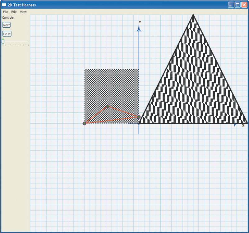
Figure 9.14: A screen capture for the texture-mapping program of Exercise 9.6, showing the texture on the left, a large triangle, and the locations of the triangle’s vertices in texture coordinates atop the texture. The resultant texturing on the triangle’s interior is shown on the right.
Exercise 9.7: Suppose that you have a polyline in the plane with vertices P0, P1, ..., Pn and you want to “resample” it, placing multiple points on each edge, equally spaced, for a total of k + 1 points Q0 = P0, ..., Qk = Pn.
(a) Write a program to do this: First compute the total length L of the polyline, then place the Qs along the polyline so that they’re separated by L/k. This will require special handling at each vertex of the original polyline.
(b) When you’re done, you’ll notice that if n and k are nearly equal, many “corners” tend to get cut off the original polyline. It’s natural to say, “I want equally spaced points, but I want them to include all the original points!” That’s generally not possible, but we can come close. Suppose that the shortest edge of the original polygon has length s. Show that you can place approximately L/s points Q0, Q1, ... on the original polyline, including all the points P0, ..., Pn, with the property that the ratio of the greatest gap between adjacent points and the smallest gap is no more than 2.
(c) Suppose you let yourself place CL/s points with the same constraints as in the previous part, for some C greater than one. Estimate the max-min gap ratio in terms of C.
Exercise 9.8: Consider the interval [p, q] where p ≠ q. If we define ![]() and
and ![]() , then α and β are called the barycentric coordinates of x.
, then α and β are called the barycentric coordinates of x.
(a) Show that for x ![]() [p, q], both α(x) and β(x) are between 0 and 1.
[p, q], both α(x) and β(x) are between 0 and 1.
(b) Show that α(x) + β(x) = 1.
![]() (c) Clearly α and β can be defined on the rest of the real line, and these definitions depend on p and q; if we call them αpq and βpq, then we can, for another interval [p′, q′], define corresponding barycentric coordinates. How are αpq(x) and αp′, q′ (x) related?
(c) Clearly α and β can be defined on the rest of the real line, and these definitions depend on p and q; if we call them αpq and βpq, then we can, for another interval [p′, q′], define corresponding barycentric coordinates. How are αpq(x) and αp′, q′ (x) related?
Exercise 9.9: Suppose you have a nondegenerate triangle in 3-space with vertices P0, P1, and P2 so that v1 = P1 – P0 and v2 = P2 – P0 are nonzero and nonparallel. Further, suppose that we have values f0, f1, f2 ![]() R associated with the three vertices. Barycentric interpolation of these values over the triangle defines a function that can be written in the form
R associated with the three vertices. Barycentric interpolation of these values over the triangle defines a function that can be written in the form
for some vector w. We’ll see this in two steps: First, we’ll compute a possible value for w, and then we’ll show that if it has this value, f actually matches the given values at the vertices.
(a) Show that the vector w must satisfy vi · w = fi – f0 for i = 1, 2 for the function defined by Equation 9.27 to satisfy f(P1) = f1 and f(P2) = f2.
(b) Let S be the matrix whose columns are the vectors v1 and v2. Show that the conditions of part (a) can be rewritten in the form
![]() (c) Explain why SST must be invertible.
(c) Explain why SST must be invertible.
(d) Show that if w is a suitable vector for Equation 9.27, then so is w + αn for any α where n = v1 × v2 is the triangle normal. We can therefore assume that we’re looking for a vector w in the plane of the triangle, i.e., one that can be written as a linear combination w = Su of the vectors v1 and v2.
(e) Write w = Su, substitute in the result of part b, and conclude that ![]() .
.
(f) Suppose that w′ = w + αn, where n = v1 × v2 is the normal vector to the triangle. Show that we can replace w with w′ in the formula for f and still have f(Pi) = fi for i = 0, 1, 2.