
Chapter 37. Spatial Data Structures
37.1. Introduction
Spatial data structures, such as the oct tree (Figure 37.1), are the multidimensional generalization of classic ordered data structures, such as the binary search tree. Because spatial data structures generally trade increased storage space for decreased query time, these are also known as spatial acceleration data structures. Spatial data structures are useful for finding intersections between different pieces of geometry. For example, they are used to identify the first triangle in a mesh that is intersected by a ray of light.
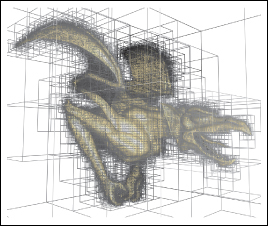
Figure 37.1: A gargoyle model embedded in an oct tree. The cube volume surrounding the model is recursively subdivided into smaller cubes, forming a tree data structure that allows efficient spatial intersection queries compared to iterating exhaustively over the triangles in the mesh. The boundaries of the cube cells are visualized as thin lines in this image. (Courtesy of Preshu Ajmera.)
The development and analysis of spatial data structures is an area in which the field of computer graphics has contributed greatly to computer science in general. The practice of associating values with locations in spaces of various dimensions is of use in many fields. For example, many machine learning, finite element analysis, and statistics algorithms rely on the data structures originally developed for rendering and animation.
The ray-casting renderer in Chapter 15 represented surfaces in the scene using an unordered list of triangles. This chapter describes how to abstract that list with an interface. Once the implementation is abstracted, we can then change that implementation without constantly rewriting the ray caster. Why would we change it? Introductory computer science courses present data structures that improve the space and time cost of common operations. In this chapter we apply the same ideas to 3D graphics scenes. Of course, when comparing 3D points or whole shapes instead of scalars, we have to adjust our notions of “greater than” and “less than,” and even “equals.”
The original ray caster could render tens of triangles in a reasonable amount of time—maybe a few minutes, depending on the image resolution and your processor speed. A relatively small amount of elegant programming will speed this up by an amazing amount. Even a naive bounding volume hierarchy should enable your renderer to process millions of triangles in a few minutes. We hope you’ll share the joy that we experienced when we first implemented this speedup. It is a great instance of algorithmic understanding leading directly to an impressive and practical result—where a small amount of algorithmic cleverness brings the miraculous suddenly to hand.
To support the generalization of 1D to k-dimensional data structures and build intuition for the performance of the spatial data structures, we first describe classic 1D ordered data structures and how they are characterized.
Because triangle meshes are a common surface representation and rays are central to light transport, data structures for accelerating ray-triangle intersection receive particular attention in this chapter and in the literature.
We select our examples from the 2D and 3D spatial data structures most commonly encountered in computer graphics. However, the structures described in this chapter apply to arbitrary dimensions and have both graphics and nongraphics applications.
Read the first half of this chapter if you are new to spatial data structures; you may want to skip it if you are familiar with the concept and are looking for details. That first half of this chapter motivates their use, explains practical details of implementing in various programming languages, and reviews evaluation methodology for data structures.
The second half of this chapter assumes that you are familiar with the concepts behind spatial data structures. It explores four of the most commonly used structures: lists, trees, grids, and hash grids. For each, a few variations are presented; for example, the BSP, kd, oct, BVH, and sphere tree variants of “trees.” The exposition emphasizes the tradeoffs between structures and how to tune a specific data structure once you have chosen to apply it.
Our experience is that it is relatively easy to understand the algorithms behind the spatial data structures, but converting that understanding to an interface and implementation that work smoothly in practice (e.g., ones that are efficient, convenient, maintainable, and general) may take years of experience.
37.1.1. Motivating Examples
Many graphics algorithms rely on queries that can be described by geometric intersections. For example, consider an animated scene containing a ball that is moving with constant velocity toward a pyramid of three boxes resting on the ground, as depicted in Figure 37.2. As the ball moves along its straight-line path, the ball traces a 3D volume called a capsule, which is a cylinder with radius equal to that of the ball and capped by two hemispheres bounding all of the trailing and leading sides of the sphere. For each discrete physical simulation time step, there is a capsule bounding all of the ball’s locations during the time. The boxes are static, so the volume that they occupy remains constant. A collision between the moving sphere and the boxes will occur during some time step. To determine if the collision is in the current step, we can compute the geometric intersection of the capsule and the boxes. If it is empty, then at no time did the ball intersect the boxes, so there was no collision. If the intersection is nonempty, then there was a collision and the dynamics system can respond appropriately by knocking over the boxes and altering the ball’s path.
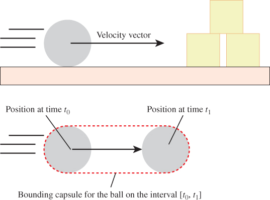
Figure 37.2: During any time interval, a sphere moving with constant velocity traces the volume of a capsule. If the intersection of the capsule and the boxes is not empty during a time interval, a collision occurred during that interval.
Intersection computation is also essential for rendering. Some common intersection queries in graphics that arise from rendering are
• The first intersection of a light ray with a scene for ray casting or photon tracing
• The intersection of the camera’s view frustum with the scene to determine which objects are potentially visible
• The intersection of a ball1 around a light source with a scene to determine which objects receive significant direct illumination from it
1. A ball is the volume inside the sphere; technically, a geometric sphere Sk is the (k – 1) dimensional surface and not the k-dimensional volume within it. However, beware that intersections with balls are casually referred to as “sphere intersections” by most practitioners.
• The intersection of a ball with a set of stored incoming photon paths to estimate radiance in photon mapping
In the dynamics example of a scene with three boxes and a single moving sphere, it would be reasonable to compute the capsule at each time step and then iterate through all boxes testing for intersections with it. That strategy for collision detection would not scale to a scene with millions of geometric primitives. Informally, to scale well, we require an algorithm that can detect a collision in fewer than a linear number of operations in the number of primitives, n. We expect that using data structures such as trees can reduce the intersection-testing costs to O(log n) in the average case, for example. The best asymptotic time performance that an algorithm could exhibit in a nontrivial case is O(m) for m actual intersections, since the intersections themselves must be enumerated. This is achievable if we place spatial distribution constraints on the input; for example, accepting an upper bound on the spatial density of primitives [SHH99]. Note that even with such constraints, m = n in the worst case, so any spatial intersection query necessarily exhibits worst-case O(n) time complexity. Furthermore, obtaining optimal performance might require more storage space or algorithmic complexity than an implementation is able to support.
There is no “best” spatial data structure. Different ones are appropriate for different data and queries. For example, finding capsule-box intersections in a scene with four primitives lends itself to a different data structure than ray-triangle intersections in a scene with millions of rays and triangles. This is the same principle that holds for classic data structures: e.g., A hash table is neither better nor worse than a binary search tree in general; they are appropriate for different kinds of applications. With spatial data structures, a list of boxes may be a good fit for a small scene. For a large scene, a binary space partition tree may be a better choice.
The art of algorithm and system design involves selecting among alternative data structures and algorithms for a specific application. In doing so, one considers the time, space, and implementation complexity in light of the input size and characteristics, query frequency, and implementation language and resources. The rest of this chapter explores those issues.
37.2. Programmatic Interfaces
Spatial data structures are typically implemented as polymorphic types. That is, each data structure is parameterized on some primitive type that in this chapter we’ll consistently name Value. For example, in most programming languages you don’t just instantiate a list; instead, you make a list of something. These are known as templated classes in C++ and C# and generics in Java. Languages like Scheme, Python, JavaScript, and Matlab rely on runtime dynamic typing for polymorphic types, and languages like ML use type inference to resolve the polymorphism at compile time. The three popular graphics OOP languages Java/C++/C# use angle-bracket notation for this polymorphism, so we adopt it too (e.g., List<Triangle> is the name of a structure representing a list of triangles).
Throughout this chapter, we assume that Value is the type of the geometric primitive stored in the data structure. Common primitive choices include triangle, sphere, mesh, and point. A value must support certain spatial queries in order to be used in building general spatial data structures. We describe one scheme for abstracting this in Section 37.2.2.2. Briefly, a data structure maps keys to values. For a spatial data structure the keys are geometry and the values are the properties associated with that geometry. One frequently implements the key and value as different interfaces for the same object through some polymorphic mechanism of the implementation language. For example, a building object might present a rectangular slab of geometry as a key for arrangement within a data structure but also encodes as a value information about its surface materials, mass, occupants, and replacement cost for simulation purposes. Note that depending on the application, the key might assume radically different forms, such as a finely detailed mesh, a coarse bounding volume on the visible geometry, or even a single point at the center of mass for simulation purposes. The same value may be represented by different keys in different data structures, but extracting a specific class of key from a value must be a deterministic process for a specific data structure.
Beware that the use of the data-structure term “key” here is consistent with the general computer science terminology employed throughout the chapter, but it is uncommon in typical graphics usage. Instead, keys that are volumes are often called bounding geometry, bounding volumes [RW80], or proxies.
In this chapter, we use the variable name key to represent whatever form of geometric key is employed by the data structure at that location in the implementation. The type of the key depends on the data structure and application. We also use the name value, which will always have class Value.
In terms of an application interface, the methods implementing the intersection queries may be framed precisely to return the geometric intersections (see Figure 37.3, left) or conservatively to return all primitives containing the intersection geometry (see Figure 37.3, right). The latter is important because the intersections between simple shapes may be hard to represent efficiently. For example, consider the intersection of a set of triangles with a ball about a point light. The intersection probably contains many triangles that are cut by the surface of the ball. The resultant shapes are not representable as triangles. However, the rendering system that will use this information likely operates on triangles, since that was the representation chosen for the underlying scene. Creating a representation for triangles-cut-by-curves will create complexity in the system that only results in shapes that the renderer can’t directly process anyway. In this case, a conservative query that returns all triangles that intersect the ball is more useful than a precise query that returns the geometric intersection of the scene and the ball.
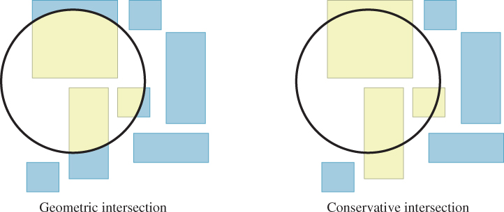
Figure 37.3: (Left) The geometric intersection of a ball with a set of boxes in 2D. (Right) A conservative result that may be more efficient to compute.
To make the structures useful, traditional set operations such as insert, remove, and is-member are generally provided along with geometric intersection. The algorithms for those tend to be straightforward applications of nonspatial data structure techniques. In contrast, the intersection queries depend on the geometry. They are the core of what makes spatial data structures unique, so we’ll focus on those.
37.2.1. Intersection Methods
Some of the most common methods of spatial data structures are those that are used to find the intersection of a set of primitives with a ball (the solid interior bounded by a sphere), an axis-aligned box, and a ray. Listing 37.1 gives a sample C++ interface for these.
Listing 37.1: Typical intersection methods on all spatial data structures.
1 template<class Value>
2 class SpatialDataStructure {
3 public:
4 void getBallIntersection (const Ball& ball, std::vector<Value*>& result) const;
5 void getAABoxIntersection(const AABox& box, std::vector<Value*>& result) const;
6 bool firstRayIntersection(const Ray& ray, Value*& value, float& distance) const;
7 };
There are of course many other useful intersection queries, such as the capsule-box intersection from the collision detection example. For an application in which a particular intersection query occurs very frequently and affects the performance of the entire system, it may be a good idea to implement a data structure designed for that particular query.
In other cases, it may make more sense to perform intersection computations in two passes. In that case, the first pass leverages a general spatial data structure from a library to conservatively find intersections against some proxy geometry. The second pass then performs exhaustive and precise intersection testing against only the primitives returned from the first query. For the right kinds of queries, this combines the performance of the sophisticated data structure with the simplicity of list iteration.
For example, dynamics systems often step through short time intervals compared to the velocities involved, so the capsule swept by a moving ball may in fact not be significantly larger than the original ball. It can thus be reasonably approximated by a ball that encloses the entire capsule, as shown in Figure 37.4.

Figure 37.4: Approximating a short capsule (dashed line) with a bounding ball (solid line). To satisfy persistence of vision, the rendering frame rate for an animation is usually chosen so that objects move only a fraction of their own extent between frames. In this case, a static bounding ball around the path of a dynamic ball is not too conservative.
A generic ball-box intersection finds all boxes that are near the capsule, including some that may not actually intersect the capsule. If there are few boxes returned from this query, simply iterating through that set is efficient. In fact, the two-pass operation may be more efficient than a single-pass query on a special-purpose data structure for capsule-box intersection. This is because the geometric simplicity of a ball may allow optimizations within the data structure that a capsule may not admit.
Like a ball, an axis-aligned box and a ray have particularly simple geometry. Thus, while our three sample intersection query methods motivate the design patterns that could be applied to alternative query geometry, they are often good choices in themselves.
Some careful choices in the specifications of intersection query methods can make the implementation and the application particularly convenient. We now detail a particular specification as an example of a useful one for general application. Consider this as a small case study of some issues that can arise when designing spatial data structures, and add the solutions to your mental programmer’s toolbox.
You may follow the exact specification given here at some point, but more likely you will apply these ideas to a slightly different specification of your own. You will also likely someday find yourself using someone else’s spatial data structure API. That API will probably follow a different specification. Your first task will be to understand how it addresses the same issues under that specification, and how the differences affect performance and convenience.
Method getBallIntersection,
1 void getBallIntersection
2 (const Ball& ball,
3 std::vector<Value*>& result) const;
appends all primitives that overlap (intersect) the ball onto the result array.2 It does not return the strict intersection itself, which would require clipping primitives to the ball in the general case.
2. In this chapter, “array” denotes a dynamic array data structure (e.g., std::vector in C++) to distinguish that concept from geometric vectors.
Appending to, rather than overwriting, the array allows the caller more flexibility. If the caller requires overwrite behavior, then it can simply clear the array itself before invoking the query. Some tasks in which overwriting is undesirable are accumulating the results of several queries, and applying the same query to primitive sets stored in different data structures.
We assume getBallIntersection returns only primitives that overlap the ball. The primitives stored in the data structure may contain additional information that is unnecessary for the intersection computation, such as reflectivity data for rendering or a network connection for a distributed application like a multi-player game. They may also present different geometry to different subsystems. Thus, while a data structure may make conservative approximations for efficiency, it must ultimately query the primitive to determine exact intersections. Querying the primitives may be relatively expensive compared to the conservative approximations. An alternative interface to the ball intersection routine would return a conservative result of primitives that may overlap the ball, using only the conservative tests. This is useful, for example, if the caller intends to perform additional intersection tests on the result anyway.
Method getAABoxIntersection,
void getAABoxIntersection(const AABox& box, std::vector<Value*>& result) const;
is similar to getBallIntersection. It finds all primitives in the data structure that overlap the interior of the axis-aligned box named box. Overlap tests against an axis-aligned box are often significantly faster than those performed against an arbitrarily oriented box, and the box itself can be represented very compactly.
The use of axis-aligned boxes is important for more than primitive intersections. For data structures such as the kd-tree and grid that contain spatial partitions aligned with the axes, the axis-aligned box intersection against internal nodes in a data structure may be particularly efficient and implemented with only one or two comparisons per axis.
Method firstRayIntersection,
bool firstRayIntersection(const Ray& ray, Value*& value, float& distance) const;
tests for intersections between the primitive set and a ray (Figure 37.5). There are three possible results.
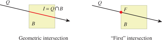
Figure 37.5: (Left) The geometric intersection I of a 2D query ray Q with box B. (Right) The point F that we call the first intersection between the ray and box, that is, the point on the geometric intersection that is closest to the ray origin.
1. There is no intersection. The method returns false and the referenced parameters are unmodified.
2. The intersection closest to the ray origin is at distance r and r ≥ distance. The method returns false and the referenced parameters are unmodified.
3. The intersection closest to the ray origin is at distance r < distance. The method returns true. Parameter distance is overwritten with r and value is a pointer to the primitive on which the intersection lies.
This interface is motivated by the common applications of the query method, such as the one from Listing 37.2. For example, consider the cases of ray casting for eye rays, light rays (photons), moving particles, or picking (a.k.a. selecting) an object whose projection lies under a mouse pointer. In each case, there may be many objects that have a nonzero intersection with the ray, but the caller only needs to know about the one producing the intersection closest to the ray origin. These objects might be stored in multiple data structures—perhaps distinguishing static and dynamic objects or ones whose different geometry is better suited to different data structures. Given an intersection query result from one data structure, the query to the second data structure need not search any farther than the previously found intersection. The caller almost always will overwrite the previously closest-known distance, so it makes sense to simply update that in place. Listing 37.2 demonstrates a terse yet readable implementation of this case. Note that there’s potential for a subtle bug in this code—if the second ray intersection were accidentally written as hit = hit || dynamicObjects..., then any intersection with a static object would preclude ever testing for a closer intersection with a dynamic object. Misuse of the early-out behavior of the logical OR operator is a danger not limited to ray intersection or computer graphics, of course!
Listing 37.2: Typical application of FirstRayIntersection in a ray-tracing renderer.
1 Radiance rayTrace(const Ray& ray) {
2 float distance = INFINITY;
3 Value* ptr = NULL;
4
5 bool hit = staticObjects.firstRayIntersection (ray, ptr, distance);
6 hit = dynamicObjects.firstRayIntersection(ray, ptr, distance) || hit;
7
8 if (hit) {
9 return shade(ptr, ray.origin + distance* ray.direction);
10 } else {
11 return Radiance(0);
12 }
13 }
Even when the high-level scene management code creates only one spatial data structure, there are likely many spatial data structures in the program. This is because, like any other sophisticated data structures, complex spatial data structures tend to be implemented using multiple instances of simpler spatial data structures. For example, the contents of each node in a spatial tree are typically stored in a spatial list, and the child subtrees of that node are simply other instances of spatial trees. Intersection methods like the ones proposed here that are designed to accumulate the results from multiple structures make it easy to design complex spatial data structures.
In addition to the convenience for the caller of passing a distance limit that will be updated, there are some applications for which there is inherently some limit to how far the caller wants to search. Examples include picking with a range-limited virtual tool or casting a shadow ray to a light source. Communicating the search limit to the data structure allows it to optimize searching for the intersection.
For ray-triangle intersection, firstRayIntersection is often extended to return the barycentric coordinates of the intersection location on the triangle hit. As described in Section 9.2, these three weights are sufficient to reconstruct both the location on the triangle where the ray first intersects it and any shading parameters interpolated from the vertices of the triangle. Returning the barycentric coordinates is not necessary because, given the distance along the ray to the intersection, the caller could reconstruct them. However, they are naturally computed during the intersection computation, so it is efficient and convenient to pass them back to the caller rather than imposing the cost of recomputing them outside the query operation.
Some data structures can resolve the query of whether any intersection exists for r < distance faster than they can find the closest one. This is useful for shadow and ambient occlusion ray casting. In that case a method variant that takes no value parameter and does not update distance is a useful extension.
37.2.2. Extracting Keys and Bounds
![]() We want to be able to make data structures that can be instantiated for different kinds of primitives. For example, a tree of triangles and a tree of boxes should share an implementation. This notion of the tree template as separate from a specific type of tree is called polymorphism. It is something that you are probably very familiar with from classic data structures. For example,
We want to be able to make data structures that can be instantiated for different kinds of primitives. For example, a tree of triangles and a tree of boxes should share an implementation. This notion of the tree template as separate from a specific type of tree is called polymorphism. It is something that you are probably very familiar with from classic data structures. For example, std::vector<int> and std::vector<std::string> share an implementation but are specialized for different value types.
For spatial data structures, we therefore require some polymorphic interface both for each data structure and for extracting a key from each Value. The choice of interface depends on the implementation language and the needs of the surrounding program.
37.2.2.1. Inheritance
In an object-oriented language such as Java, one typically uses inheritance to extract keys, as shown in Listings 37.3 and 37.4 (the latter listing has the example).
Listing 37.3: A Java inheritance interface for expressing axis-aligned bounding box, sphere, and point keys on a primitive and responding to corresponding conservative intersection queries.
1 public interface Primitive {
2 /** Returns a box that surrounds the primitive for use in
3 building spatial data structures. */
4 public void getBoxBounds (AABox bounds);
5
6 public void getSphereBounds (Sphere bounds);
7
8 public void getPosition (Point3 pos);
9
10
11 /** Returns true if the primitive overlaps a box for use
12 in responding to spatial queries. */
13 public bool intersectsBox (AABox box);
14
15 public bool intersectsBall (Ball ball);
16
17 /** Returns the distance to the intersection, or inf if
18 there is none before maxDistance */
19 public float findFirstRayIntersection(Ray ray, float maxDistance);
20 }
21
22 public class SomeStructure<Value> {
23 ...
24 void insert(Value value) {
25 Point3 key = new Point3();
26 value.getPosition(key);
27 ...
28 }
29 }
Listing 37.4: One possible implementation of a triangle under an inheritance-based scheme. The getBoxBounds implementation computes the bounds as needed; an alternative is to precompute and store them.
1 public class Triangle implements Primitive {
2
3 private Point3 _vertex[3];
4
5 public Point3 vertex(int i) {
6 return _vertex[i];
7 }
8
9 public void getBoxBounds(AABox bounds) {
10 bounds.set(Point3::min(vertex[0], vertex[1], vertex[2]),
11 Point3::max(vertex[0], vertex[1], vertex[2]));
12 }
13 ...
14
15 }
Inheritance is usually well understood by programmers working in an object-oriented language. It also keeps the implementation of program features related to a Value within that Value’s class. This makes it a very attractive choice for extracting keys. The simplicity comes at a cost in flexibility, however. Using an inheritance approach, one cannot associate two different key extraction methods with the same class, and the needs of a spatial data structure impose on the design of the Value class, forcing them to be designed concurrently.
37.2.2.2. Traits
A C++ implementation might use a trait data structure in the style of the design of the C++ Standard Template Library (STL). In this design pattern, a templated trait class defines a set of method prototypes, and then specialized templates give implementations of those methods for particular Value classes. Listing 37.5 shows an example of one such interface named PrimitiveKeyTrait that supports box, ball, and point keys. Below that definition is a specialization of the template for a Triangle, and an example of how a spatial data structure would use the trait class to obtain a position key from a value.
Listing 37.5: A C++ trait for exposing axis-aligned bounding box, sphere, and point keys from primitives.
1 template<class Value>
2 class PrimitiveKeyTrait {
3 public:
4 static void getBoxBounds (const Value& primitive, AABox& bounds);
5 static void getBallBounds (const Value& primitive, Ball& bounds);
6 static void getPosition (const Value& primitive, Point3& pos);
7
8 static bool intersectsBox (const Value& primitive, const AABox& box);
9 static bool intersectsBall(const Value& primitive, const Ball& ball);
10 static bool findFirstRayIntersection(const Value& primitive, const Ray& ray,
float& distance);
11 };
12
13 template<>
14 class PrimitiveKeyTrait<Triangle> {
15 public:
16 static void getBoxBounds(const Triangle& tri, AABox& bounds) {
17 bounds = AABox(min(tri.vertex(0), tri.vertex(1), tri.vertex(2)),
18 max(tri.vertex(0), tri.vertex(1), tri.vertex(2)));
19 }
20 ...
21 };
22
23 template< class Value, class Bounds = PrimitiveKeyTrait<Value> >
24 class SomeStructure {
25 ...
26 void insert(const Value& value) {
27 Box key;
28 Bounds<Value>::getBoxBounds(value, key);
29 ...
30 }
31 };
Overloaded functions are a viable alternative to partial template specialization in languages that support them. An example of providing an interface through overloading in C++ is shown in Listing 37.6. This is similar to the template specialization, but is a bit more prone to misuse because some languages (notably C++) dispatch on the compile-time type instead of the runtime type of an object. (ML is an example of a language that dispatches on runtime type.) If mixed with inheritance, overloading can thus lead to semantic errors.
Listing 37.6: A C++ trait implemented with overloading instead of templates.
1 void getBoxBounds(const Triangle& primitive, AABox& bounds) { ... }
2 void getBoxBounds(const Ball& primitive, AABox& bounds) { ... }
3 void getBoxBounds(const Mesh& primitive, AABox& bounds) { ... }
4 ...
5
6 template<class Value>
7 class SomeStructure {
8 ...
9 void insert(const Value& value) {
10 Box key;
11 // Automatically finds the closest overload
12 getBoxBounds(value, key);
13 ...
14 }
15 };
Traits can also be implemented at runtime in languages with first-class functions or closures. This forgoes static type checking but allows the flexibility of the design pattern with less boilerplate and in more languages. For example, Listing 37.7 uses the trait pattern in Python and depends on dynamic typing and runtime error checks to ensure correctness.
Listing 37.7: A Python trait for exposing axis-aligned bounding box, sphere, and point keys from primitives.
1 def getTriangleBoxBounds(triangle, box):
2 box = AABox(min(tri.vertex(0), tri.vertex(1), tri.vertex(2)),
3 max(tri.vertex(0), tri.vertex(1), tri.vertex(2)))
4 }
5
6 class SomeStructure:
7 _bounds = null
8
9 def __init__(self, boundsFunction):
10 self._bounds = boundsfunction
11
12 ...
13 def insert(self, value):
14 Box key;
15 self._bounds(value, key)
16 ...
17 }
18 };
19
20 SomeStructure s(getTriangleBoxBounds)
The trait design pattern for extracting keys has three main advantages. Traits allow the data structure implementor to make the data structure work with Value classes that predate it. For example, you can create your own new binary space partition tree spatial data structure and write a trait to make it work with the Triangle class from an existing library that you cannot modify. A related advantage is that traits move the complexity of the key-extraction operation out of the Value class.
Another advantage of traits is that they allow instances of data structures with the same Value to use different traits. For example, you may wish to build one tree that uses the vertex of a triangle that is closest to the origin as its position key, and another that uses the centroid of the triangle as its position key. However, if getPositionKey is a method of Triangle, then this is not possible. Under the pattern shown in Listing 37.5, these would be instantiated as SomeStructure<Triangle, MinKey> and SomeStructure<Triangle, CentroidKey>.
A disadvantage of traits compared to inheritance is that traits separate the implementation of a Value class into multiple pieces. This can increase the cost of designing and maintaining such a class.
Traits also involve more complicated semantics and syntax than other approaches. This is particularly true for the variant shown in Listing 37.5 that uses C++ templates. Many C++ programmers have never written their own trait-based classes, or even their own templated classes. Almost all have used templated classes and traits, however. So this design pattern significantly increases the barrier to creating a new kind of data structure and slightly increases the barrier to creating a new kind of primitive, but introduces little barrier to using a data structure.
Overall, we find the trait design necessary in practice for efficiency and modularity, but we regret the modularity lost in Value classes. We regard traits as a necessary evil in practice.
37.3. Characterizing Data Structures
![]() Classic ordered structures contain a set of elements. Each element has value and a single integer or real number key. For example, the values might be student records and the keys the students’ grades. We say that the data structures are ordered because there is a total ordering on the keys.
Classic ordered structures contain a set of elements. Each element has value and a single integer or real number key. For example, the values might be student records and the keys the students’ grades. We say that the data structures are ordered because there is a total ordering on the keys.
Regardless of their original denotation, one can interpret the key as a position on the real number line. This leads to our later generalization of multidimensional keys representing points in space.
There are many ways to analyze data structures. In this chapter, you’ll see two kinds of analysis intermixed. It is impossible to give a one-size-fits-all characterization of these structures and advice on which is “best”—it depends on the kind of data you expect to encounter in the scene. We therefore sketch asymptotic analyses and offer practical considerations of how they apply to real use. The conclusions of each section aren’t really the goal. Instead, the issues raised in the course of reaching them are what we want you to think about and apply to problems.
We do recognize two usage patterns and prescribe the following high-level advice in selecting data structures.
• When using data structures in a generic way, trust asymptotic bounds (“big-O”). Generic use means for a minor aspect of an algorithm, for fairly large problems, and where you know little about the distribution of keys and queries. Trusting bounds means, for example, that operations on trees are often faster than on lists at comparable storage cost. Parameterize the bound on the factor that you really expect to dominate, which is often the number of elements.
• When considering a specific problem for which you have some domain knowledge and really care about performance, use all of your engineering skill. Consider the actual kinds of scenes/distributions and computer architecture involved, and perform some experiments. Perhaps for the size of problem at hand the scattered memory access for a tree is inferior to that of an array, or perhaps the keys fall into clusters that can be exploited.
To make the analysis tools concrete and set up an analogy to spatial data structures, we show an example on two familiar classic data structures in the following subsections. Consider two alternatives for storing n values that are student records in a course database at a college, where each record is associated with a real-number key that is the student’s grade in the course.
The first structure to consider is a linked list. Although we say that a list is an “ordered” data structure, recall that the description applies to the fact that any two keys have a mathematical ordering: less than, greater than, or equal to. The order of elements within the list itself will be arbitrary. More sophisticated data structures exploit the ordering of the keys to improve performance.
The second data structure is a balanced binary tree. The elements within the tree are arranged so that every element in the right subtree of a node contains elements whose keys are larger than or equal to the key at the node. The left subtree of a node contains elements whose keys are less than or equal to the key at the node.
37.3.1. 1D Linked List Example
The list requires storage space proportional to n, the number of student records. The exact size of the list is probably n times the sum of the size of one record and the size of one pointer to the next record, plus some additional storage in a wrapper class, such as the one in Listing 37.8. We describe this as the list occupying O(n) space, which means that for sufficiently large n the actual size is less than or equal to c · n for some constant c.
Concretely, consider the time cost of finding student records in the list that lie within a continuous range of grades. If we think of the records as distributed along a number line at points indicated by their keys, the find operation is equivalent to finding the geometric intersection of the desired grade interval and the set of records. This geometric interpretation will later guide us in building higher-dimensional keys, where we want to perform intersection queries against higher-dimensional shapes such as balls and boxes.
To find records intersecting the grade interval, we must examine all n records and accept only those whose keys lie within the interval. Note that because the list index is independent of the key, we must always look at all n records. There is probably some overhead time for launching the find operation and the time cost of each comparison depends on the processor architecture. These make it hard to predict the exact runtime, but we can characterize it as O(n) for a single find operation.
When employed with care, the big-O notation is useful for characterizing the asymptotic growth of the data structure without the distraction of small overhead constants. The important idea is that for lists that we are likely to encounter in practice, if we double the length of the list we approximately double the memory requirement. That is, if the list has length 100, we probably don’t care about the small overhead cost of storing a constant number of extra values.
When we are ready to implement a system, with some idea of the data’s size and capabilities of the hardware, we augment the asymptotic analysis with more detailed engineering analysis. At this stage it is important to consider the impact of constant space and time factors. For example, say that our list stores a few kilobytes of data in addition to the records. This might be information about a freelist buffer pool for fast memory allocation, the length of the list, and an extra pointer to the tail of the list for fast allocation, as described in Listing 37.8.
Listing 37.8: Sample templated list class.
1 template<class Value>
2 class List {
3 class Node {
4 public:
5 float key;
6 Value value;
7 Node* next;
8 };
9
10 Node* head;
11 Node* tail;
12 int length;
13 Node* freelist;
14 ...
15 };
Under this list representation, a list of three small elements might require almost the same amount of space as a list of six elements. For small lists, we’ll find that the length of the freelist dominates the total space cost of the list.
Under an engineering analysis we should thus extend our implementation-independent asymptotic analysis with both the constant factors and the newly revealed parameters from the implementation, such as the size of the freelist and the overhead of accessing a record.
37.3.2. 1D Tree Example
A binary search tree exploits the ordering on the keys to increase the performance of some find operations. In doing so it incurs some additional constant performance overhead for every search and increases the storage space.
The motivation for using a tree is that we’d like to be able to find all students with grades in some interval and do so faster than we could with the list. The tree representation is similar to the list, although there are two child pointers in each node. So the space bounds are slightly higher by a constant factor, but the storage cost for n elements is still O(n).
The height of a balanced binary tree of n students is ![]() log2 n
log2 n![]() . If there is only one student whose grade is in the query interval, then we can find that student using at most
. If there is only one student whose grade is in the query interval, then we can find that student using at most ![]() log2 n
log2 n![]() comparisons. Furthermore, if that student’s record is at an internal (versus leaf) node of the tree, it may take as few as three comparison operations to locate the student and eliminate all others.
comparisons. Furthermore, if that student’s record is at an internal (versus leaf) node of the tree, it may take as few as three comparison operations to locate the student and eliminate all others.
Thus, for the case of a single student in the interval, the search takes worst-case O(lg n) time, which is better than the list. In practice, the constants for iterating through a tree are similar to those for iterating through a list, so it is reasonable to expect the tree to always outperform the list.
Depending on the size of the interval in the query and the distribution of students, there may be more than one student in the result. This means that the time cost of the find operation is output-sensitive, and the size of the output appears in the bound. If there are s students that satisfy the query, the runtime of the query is necessarily O(s + lg n). Since 0 ≤ s ≤ n, in the worst case all students may be in the output. Thus, the tightest upper bound for the general case is O(n) time.
We could try to characterize the time cost based on the distribution of grades and queries that we expect. However, at that point we’re mixing our theory with engineering and we’re unlikely to produce a bound that informs either theory or practice. Once we know something about the distribution and implementation environment, we should perform back-of-the-envelope analysis with the actual specifications or start performing some experiments.
At a practical level, we might consider the cache coherence implications of chasing tree pointers through memory versus sequential access for a tree packed into an array as a vector heap, or a list packed into an array. We might also look at the complexity of the data structure and the runtime to build and update the tree to support the fast queries.
In the case where queries and geometry are unevenly distributed, balancing the tree might not lead to optimal performance over many queries. For example, say that there are many students whose grades cluster around 34 but we don’t expect to query for grades less than 50 very often. In that case, we want a deep subtree for grades less than 50 so that students with grades greater than 50 can appear near the root. Nodes near the root can be reached more quickly and are more likely to stay in cache.
37.4. Overview of k-dimensional Structures
The remainder of this chapter discusses four classes of spatial data structures. These correspond fairly closely to k-dimensional generalizations of classic one-dimensional lists, trees, arrays, and hash tables under the mapping shown in Table 37.1. In that table, the actual intersection time depends on the spatial distribution of the elements and the intersection query geometry, but the big-O values provide a useful bound.
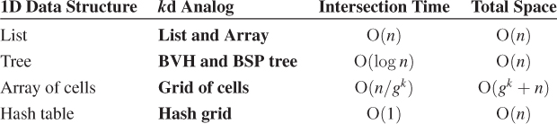
Table 37.1: Approximate time and space costs of various data structures containing n elements in k dimensions. The grids have g subdivisions per axis, which is not modeled by these expressions.
We can build some intuition for the runtimes of spatial data structures: Operations should take linear time on lists, log time on trees, and constant time on regular grids. The space requirements of a regular grid are problematic because the grid allocates memory even for areas of the scene that contain no geometry. However, using a hash table, we can store only the nonempty cells. Thus, we can expect list, tree, and hash grid structures to require only a linear amount of space in the number of primitives that they encode.
With some knowledge of the scene’s structure, one can often tune the data structures to achieve amortized constant factor speedups through architecture-independent means. These might be factors of two to ten. Those are often necessary to achieve real-time performance and enable interaction. They may not be worthwhile for smaller data sets or applications that do not have real-time constraints.
All of these observations are predicated on some informal notions of what is a “reasonable” scene and set of parameters. It is also possible to fall off the asymptotic path if the scene’s structure is poor. In fact, you can end up making computations slower than linear time. The worst-case space and time bounds for many data structures are actually unbounded. To address this, for each data structure we describe some of the major problems that people have encountered. From that you’ll be able to recognize and address the common problems. That is, the time and space bounds given in the table are only to build intuition for the general case. As discussed in the previous section, one has to assume certain distributions and large problems to prove these bounds, and doing so is probably reductive. Understanding your scenes’ geometry distributions and managing constant factors are important parts of computer graphics. Concealing those behind assumptions and abstractions is useful when learning about the data structures. Rolling back assumptions and breaking those mathematical abstractions are necessary when applying the data structures in a real implementation.
In addition to algorithmic changes and architecture-independent constant-factor optimizations, there are some big (maybe 50x over “naive” implementations) constant-factor speedups available. These are often achieved by minding details like minimizing memory traffic, avoiding unnecessary comparisons, and exploiting small-scale instruction parallelism. Which of these micro-optimizations are worthwhile depends on your target platform, scenes, and queries, and how much you are willing to tailor the data structure to them. We describe some of the more timeless conventional wisdom accumulated over a few decades of the field’s collective experience. Check the latest SIGGRAPH course notes, EGSR STAR report, and books in series like GPU Pro for the latest advice on current architectures.
37.5. List
A 1D list is an ordered set of values stored in a way that does not take advantage of the keys to lower the asymptotic order of growth time for query operations. For instance, consider the example of a mapping from student grades to student records encoded as a linked list that is described in Section 37.3.1. Each element of the list contains a record with a grade and other student information. Searching for a specific record by grade takes n comparisons for a list of n records if they are unordered. At best, we could keep the list sorted on the keys and bring this down to expected n/2 comparisons, but it is still linear and still has a worst case of n comparisons.
For the unsorted 1D list, there’s little distinction between the expected space and time costs of a dynamic array (see Listing 37.9) and a linked-list implementation (see Listing 37.8). For the sorted case, the array admits binary search while the linked list simplifies insertion and deletion. The array implementation is good for small sets of primitives with small memory footprints each; the linked list is a better underlying representation for primitives with a large memory footprint, and even more sophisticated spatial data structures are preferred for larger sets.
Listing 37.9: C++ implementation of a spatial list, using an array as the underlying structure.
1 template<class Value, class Trait = PrimitiveKeyTrait<Value> >
2 class List {
3 std::vector<Value> data
4
5 public:
6
7 int size() const {
8 return data.size();
9 }
10
11 /* O(1) time */
12 void insert(const Value& v) {
13 data.push_back(v);
14 }
15
16 /* O(1) time*/
17 void remove(const Value& v) {
18 int i = data.find(v);
19 if (i != -1) {
20 // Remove the last
21 data[i] = data[data.size() - 1];
22 data.pop();
23 }
24 }
25
26 ...
27 };
Now consider the implications of generalizing from a 1D key such as a grade to a higher-dimensional key such as a 2D location. Figure 37.6 shows a sample 2D data set with seven points labeled a–g and two alternative list implementations corresponding to those data.
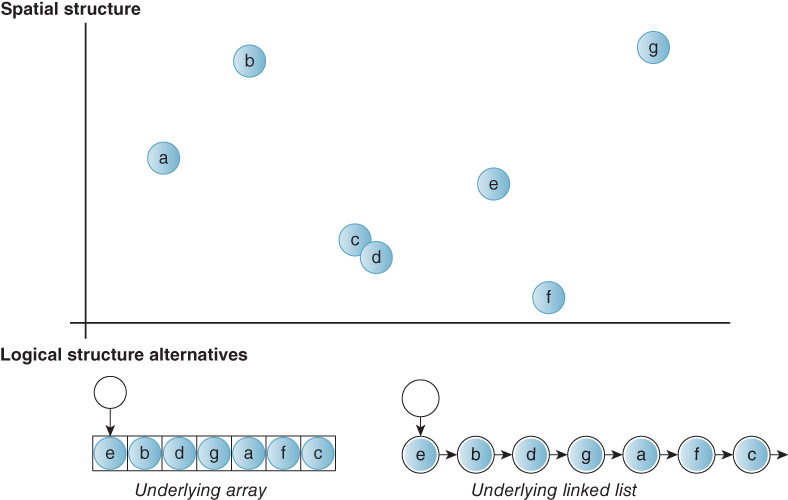
Figure 37.6: A set of points distributed in 2D and two logical data structures describing them with list semantics. The list interface on the left relies on an underlying array. The one on the right uses an underlying linked list. Note that the order of elements within the list is arbitrary.
Compared to a 1D list, there is no longer a total ordering on keys. For example, there is no general definition of “greater” between (0, 1) and (1, 0) the way that there is between 3 and 6. Note that this problem occurs because the key has two or more dimensions. There are still many cases in computer graphics where one has values that describe 3D data and associates those with 1D keys like the depth of each object in a scene from the camera. One-dimensional data structures remain as useful in graphics as in any field of computer science or software development.
Given a set of n values each paired with a kd key (Figure 37.6), a list data structure backed by a linked list or array implementation requires O(n) space. In practice, both implementations require space for more than just the n elements if the data structure is dynamic. In the linked list there is the overhead of the link pointers. A dynamic array must allocate an underlying buffer that is larger by a constant factor to amortize the cost of resizing.
Because we cannot order the values in an effective way for general queries, a query such as ray or box intersection requires n individual tests (see Listings 37.10–11). It must consider each element, even after some results that satisfy the query have been obtained. We could imagine imposing a specific ordering such as sorting by distance from the origin or by the first dimension, but unless we know that our queries will favor early termination under that sorting, this cannot even promise a constant performance improvement.
Listing 37.10: C++ implementation of ray-primitive intersection in a list. The method signature choices streamline the implementation.
1 /* O(n) time for n = size() */
2 bool firstRayIntersection(const Ray& ray, Value*& value, float& distance) const {
3 bool anyHit = false;
4
5 for (int i = 0; i < data.size(); ++i) {
6 if (Trait::intersectRay(ray, data[i], distance)) {
7 // distance was already updated for us!
8 value = &data[i];
9 anyHit = true;
10 }
11 }
12
13 return anyHit;
14 }
Listing 37.11: C++ implementation of conservative ball-primitive intersection in a list.
1 /* O(n) time for n = size() */
2 void getBallIntersection(const Ball& ball, std::vector<Value*>& result) const {
3 for (int i = 0; i < data.size(); ++i) {
4 if (Trait::intersectsBall(ray, data[i])) {
5 result.push_back(&data[i]);
6 }
7 }
8 }
Both structures allow insertion of new elements in amortized O(1) time. The linked list prefers insertion at the head and the array at the end. Finding an element to delete is a query, so it takes n operations. Once found, the linked list can delete the element in O(1) time by adjusting pointers. The array can also delete in O(1) time—it copies the last element over the one to be deleted and then reduces the element count by 1. Because the array is unordered, there is no need to copy more elements. It is critical, however, that the array and its contents be private so that there can be no external references to the now-moved last entry.
![]() There may be some advantage to the array’s packing of values in a cache-friendly fashion, but only if the elements are small. If the values are large, then they may not fit in cache lines anyway, and the cost of copying them during insertion and removal may dwarf the main memory latency and bandwidth savings.
There may be some advantage to the array’s packing of values in a cache-friendly fashion, but only if the elements are small. If the values are large, then they may not fit in cache lines anyway, and the cost of copying them during insertion and removal may dwarf the main memory latency and bandwidth savings.
37.6. Trees
Just as they do for sorted data in one dimension, trees provide substantial speedups in two or more dimensions. In 1D, “splitting” the real line is easy: We consider all numbers greater than or less than some splitting value v. In higher dimensions, we generally use hyperplanes for dividing space, and different choices for hyper-planes lead to different data structures, some of which we now describe.
37.6.1. Binary Space Partition (BSP) Trees
A 1D binary search tree recursively separates the number line with splitting points, as depicted in Figures 37.7 and 37.8. In 2D, a spatial tree separates 2-space with splitting lines, as depicted in Figure 37.9. In 3D, a spatial tree separates 3-space with splitting planes.
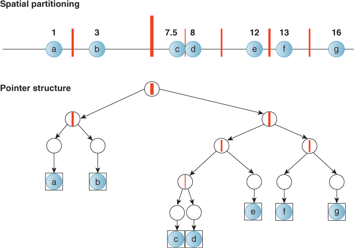
Figure 37.7: A depiction of a 1D binary tree as partitions (black lines) of values with associated keys (red disks). The thickness of the partition line represents the tree depth of that partition node in the tree; the root is the thickest.
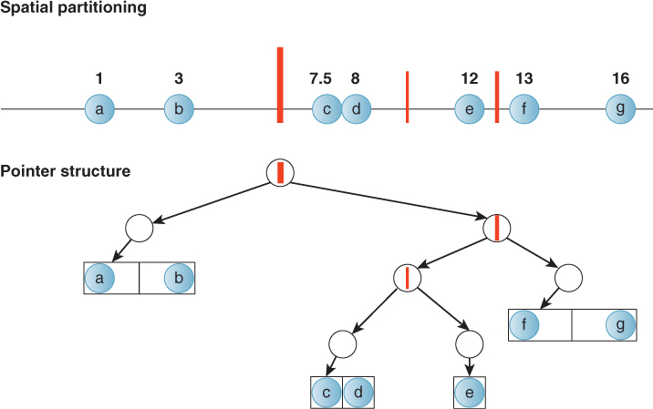
Figure 37.8: An alternative choice of tree structure for the same data shown in Figure 37.7. This tree is shallower and contains multiple primitives per node, indicated by adjacent boxes. Such a structure might be preferred if the overhead of processing a node is high.
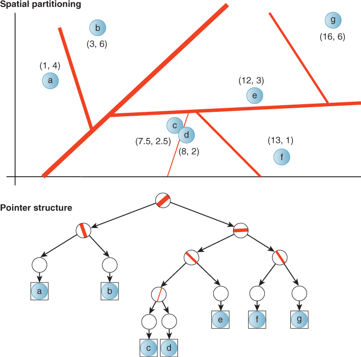
Figure 37.9: A depiction of a 2D binary space partition tree (BSP) as partitions (black lines) of values with associated keys (red disks). The thickness of the partition line represents the tree depth of that partition node in the tree; the root is the thickest.
The analogy continues to higher dimensions. For any number of dimensions, a binary space partition (BSP) tree expresses a recursive binary (i.e., two-sided) partition (i.e., division) of space [SBGS69, FUCH80]. This partitioning divides space into convex subspaces, that is, convex polygons, polyhedra, or their higher-dimensional analogs, called polytopes. The leaves of the tree correspond to these subspaces, which we’ll call polyhedra in general. The internal nodes correspond to the partition planes. They also represent convex spaces that are unions of their children.
BSP trees can support roughly logarithmic-time intersection queries under appropriate conditions. These intersection queries can be framed as intersecting some query geometry with either the convex polyhedra corresponding to the leaves, or the primitives inside the leaves. In the latter case, note that the tree is only accelerating the intersection computation on nodes. For primitives stored within a node, it delegates the intersection operation to a list data structure. That provides no further acceleration. But it allows the tree to have an interface that is more useful to an application programmer. The application programmer is primarily concerned with the primitives, and wants the tree’s structure to provide acceleration but have no semantic impact on the query result.
In addition to the ray, box, and ball queries, BSP trees can also enumerate their elements in front-to-back overlap order relative to some reference point, and they can produce a convex polyhedron bounding the empty space around a point. Many video games use the latter operation to locate the convex space that contains the viewer for efficient access to precomputed visible-surface information.
The ordered enumerations are possible because the partitions impose an ordering of the convex spaces along a ray. This allows partially ordered enumeration of primitives encountered along a ray. It is not a total ordering because some nodes may contain more than one primitive in an unordered list. The ordering of nodes allows early termination when ray casting, which is why they have been frequently employed for accelerating ray casting as described in Section 36.2.1. It also allows hierarchical culling of occluded nodes within a camera frustum and early termination in that case, as explained in Section 36.7.
The logical (i.e., pointer) structure of the tree in memory is simply that of a binary tree (see Listing 37.12), regardless of the number of spatial dimensions. Trees are typically built over primitives, such as polygons. This leaves a design choice of how to handle primitives that span a partition. In one form, primitives that span a partition plane are cut by the plane, and the leaves store lists of the cut primitives that lie entirely within their convex spaces. To preserve the precision of the input, the cutting operation may be performed while building the tree and the original primitives stored at the leaves. Under that scheme, the same primitive may appear in multiple leaves.
An alternative is to store primitives that span a partition plane in the node for that plane. This can destroy the asymptotic efficiency of the tree if many primitives span a plane near the root of the tree. However, for some scenes this problem can be avoided by choosing the partitions to avoid splitting primitives.
Listing 37.12: A C++ implementation of a binary space partition tree.
1 template<class Value, class Bounds = PrimitiveKeyTrait<Value> >
2 class BSPTree {
3 class Node {
4 public:
5 Plane partition;
6
7 /* Values at this node */
8 List<Value, Bounds> valueArray;
9
10 Node* negativeHalfSpace;
11 Node* positiveHalfSpace;
12 };
13
14 Node* root;
15
16 ...
17 };
Although all leaves represent convex spaces, the ones at the spatial extremes of the tree happen to correspond to spaces with infinite volume. For example, the rightmost space on the number line in Figure 37.7 represents the interval from 14.5 to positive infinity. Infinite volume can be awkward for some computations. It is also a strength of the tree data structure because every BSP tree can represent all of space. Thus, without even changing the structure of the tree, one can dynamically add and remove primitives from nodes. This is useful for expressing arbitrary movement of primitives through a scene. For scenes dominated by static geometry, this is a significant advantage that the tree holds over other spatial data structures such as grids that represent only finite area. Those data structures must change structure when a primitive moves outside the former bounds of the scene.
A tree containing n primitives must store at least references to all of the primitives, so its size must be at least linear in n. The smallest space behavior occurs when the tree has a small number of nodes storing a large number of primitives. It also occurs when building a highly unbalanced tree at which most nodes have only one branch, as shown in Figure 37.10.
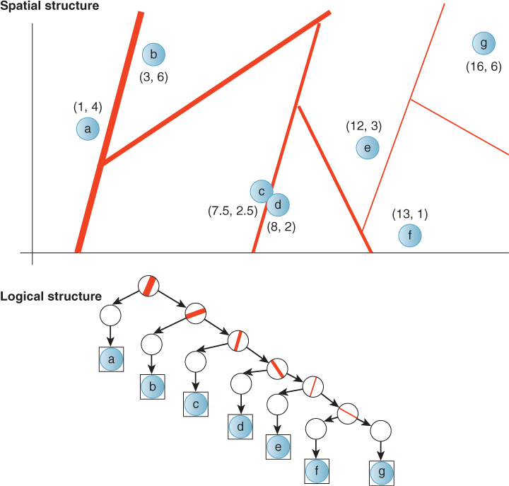
Figure 37.10: A degenerate BSP tree with the same asymptotic performance as a list. The poor performance results from an ineffective choice of partitions. This situation can arise even with a good tree-building strategy if elements move after the partitions have been placed. Even worse trees exist—there could be many empty partitions.
It is important to note that the size of the tree has no upper bound. There are two reasons for this, both of which can easily occur in practice. First, one can add partitions independent of the number of primitives. This may be useful if one expects additional primitives to be inserted later. This may occur naturally from an implementation that chooses not to remove nodes when primitives move out of them (e.g., for time efficiency in move and delete operations).
Second, in an implementation that splits primitives, poor choice of partition planes can significantly amplify the number of primitives stored. As discussed in Section 37.6.2, choosing partitions is a hard problem. For arbitrary scenes there is no reason to expect that the partitions can be chosen to avoid substantial amplification of primitives. Since sufficient amplification of the number of primitives can cancel any benefit from efficient structure, one must be careful when choosing the partition planes.
Most algorithms on trees assume that they have been built reasonably, with fewer than 2n nodes.
A balanced BSP tree can locate the leaf containing a point in O(lg n) comparisons, which is why it is common to think of tree operations as being log-time. If the tree is unbalanced but has reasonable size, this may rise as high as O(n) comparisons, as in the degenerate tree shown in Figure 37.10. For a tree with an unreasonable size there is no upper bound on the time to locate a point, just as there is no bound on the size of the tree.
Our common intersection problems—first-ray intersection, conservative ball intersection, and conservative box intersection—are all at least as hard as locating the convex region containing a point. So all intersection queries on the BSP tree take at least logarithmic expected time for a balanced tree, yet have no upper bound on runtime if the tree structure is poor. The volume (i.e., ball and box) queries are also necessarily linear in the size of the output, which can be as large as n.
The actual runtime observed for intersection queries generally grows as the amount of space covered by the query geometry increases. Fortunately, it usually grows sublinearly. The basic idea is that if a ray travels a long distance before it strikes a primitive, it probably passed through many partitions, and if it travels a short distance, it probably passed through few. The same intuition holds for the volume of primitives.
A good intuition is that the runtime might grow logarithmically with the extent of the query geometry, since for uniformly distributed primitives we would expect partitions to form a balanced tree. However, one would have to assume a lot about the distribution of primitives and partitions to prove that as a bound.
The idea of the spatial distribution of primitives is very important to the theory supporting BSP trees, despite its confounding effects on formal analysis. One typically seeks to maintain a classic binary search tree in a balanced form to minimize the length of the longest root-to-leaf path and thus minimize the expected worst-case search behavior.
Balance (and big-O analysis) helps to minimize the worst-case runtime. But under a given pattern of queries and scene distribution, you might want to find the tree structure that minimizes the overall runtime. While your algorithms book stresses the first one, what actually matters in practice is the second one.
For example, a balanced spatial data structure tree is rarely optimal in practice [Nay93]. This at first seems surprising—classic binary tree data structures are usually designed to maintain balance and thus minimize the worst case. However, since the average-case performance depends on the queries and we expect many queries for a graphics application, we should intentionally unbalance the tree to favor expected queries. This is directly analogous to the tree used to build a Huffman code for data compression. There, one knows the statistics of the input stream and wants to build a tree that minimizes the average node depth weighted by the number of occurrences of each node in the input stream. Unfortunately, we don’t know the exact queries that will be made, so we can’t apply Huffman’s algorithm exactly to building a spatial data structure. But we can choose some reasonable heuristics because our values have a spatial interpretation. For example, we might assume that queries will be equally distributed in space or that the probability of a random query returning a primitive is proportional to the size of that primitive.
Finally, because wall-clock time is what matters for this kind of analysis, we have to factor in the tree-build time and the relative costs of memory operations and comparisons when optimizing.
37.6.2. Building BSP Trees: oct tree, quad tree, BSP tree, kd tree
It is hard to choose good partition planes. There are theoretically infinitely many planes to choose from. The choice depends on the types of queries, the distribution of data, and whether one wants to optimize the worst case, the best case, or the “average” case. If the tree structure will be precomputed, the build process can be made expensive—and some algorithms take O(n2) time to build a tree on n primitives. If the tree will be built or modified frequently inside an interactive program, it is important to minimize the combination of tree-build and query time, so one might choose partitions that can be identified quickly rather than ones that give optimal query behavior.
To address the problem of considering too many choices of partition planes, it is often easier to introduce constraints so as to consider a smaller number of options. This has the added advantage of requiring fewer bits to represent the partitions, which translates to reduced storage cost and reduced memory bandwidth during queries.
One such artificial constraint is to consider only axis-aligned partitions [RR78]. The resultant BSP tree is called a kd tree (also written as “k-d tree”). The axis to split along may be chosen based on the data, or simply rotated in round-robin fashion. In the latter case, each partition plane can be represented (see Listing 37.13) by a single number representing its distance from the origin, since the plane normal is determined by the depth of a plane’s node in the tree.
Listing 37.13: kd tree representation.
1 template<class Value>
2 class KDTree {
3 class Node {
4 public:
5 float partition;
6 Node* negativeHalfSpace;
7 Node* positiveHalfSpace;
8 List<Value> valueArray;
9 };
10
11 Node* root;
12
13 ...
14 };
Regardless of restrictions, there are still many choices of where to place a partition:
• Mean split on extent
• Mean split on primitives
• Median split on primitives
• Constant ray intersection probability [Hav00]
• Clustering
Splitting along the mean of the extent of all primitives at a node along each axis yields a set of nested k-cubes [RR78]. That is, each partition is at the center of its parent’s polyhedron. In 3D, this is called an oct tree (a.k.a. “octree”) (see Listing 37.14). Although they can be represented using binary trees, for efficiency oct trees are typically implemented with eight child pointers, hence their names. They have 2D analogs in quad trees (see Figure 37.11), and can of course be extended to 1D or 4D spaces and higher.
Listing 37.14: Oct tree representation.
1 template<class Value>
2 class OctTree {
3 class Node {
4 public:
5 Node* child[8];
6 List<Value> valueArray;
7 };
8
9 Node* root;
10 Vector3 extent;
11 Point3 origin;
12 ...
13 };
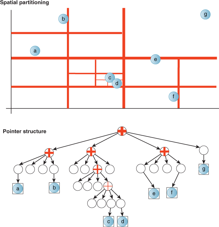
Figure 37.11: A quad tree. If a cluster of data points is not split by a low power-of-two plane position, the tree may become very deep, as near primitives c and d in this example. A better tree-building strategy for this particular data set would have been to make a second-level node containing two primitives, rather than subdividing until each node contained a single primitive. However, if c and d represented clusters of hundreds of primitives, no efficient tree would be possible—either many primitives would lie at each node, or there would be a long degenerate chain of internal nodes.
In general, building trees is a slow operation if implemented in a straightforward manner. It was classically considered a precomputation step. In that case, one avoided changing the structure of the tree at runtime.
However, if you are willing to complicate the tree-building process and work with a concurrent system, you can build trees fairly fast on modern machines. Lauterbach et al. [LGS+09] reported creating trees dynamically on a GPU at about half the speed of rasterization for a comparable number of polygons on that GPU. Having tree-building performance comparable to rasterization performance means that it can be performed on dynamic scenes. Furthermore, for many applications, most of the geometry in a scene does not change position between frames. In this case, only the subtrees containing dynamic elements need to be rebuilt. Fortunately, although implementing a fast tree-building system is difficult, there are libraries that implement the tree build for you.
Here are some conventional wisdom and details.
• Current hardware architectures favor very deep trees, so plan to keep subdividing down to one or two primitives per node [SSM+05].
• As discussed, we often want the tree to be unbalanced [SSM+05].
• Because of memory bandwidth and cache coherence, saving space saves runtime when constants are “small” (and we’re often in that case). So compact tree representations can lead to substantial speedups. Here are some tricks for reducing the memory footprint of internal nodes.
– Place children at adjacent locations in memory so that a single pointer can reference them.
– Use kd trees instead of BSP trees to limit the footprint of each node to a single offset, or oct trees so that no per-node information is required.
– Pack per-node values (such as the kd tree plane offset) directly into unused bits of the child pointer value by limiting the precision for each.
These kinds of optimizations can lead to a 10x performance increase in practice [SSM+05].
• Be careful about precision when splitting elements. Due to finite precision, the new vertices introduced will rarely lie on a splitting plane, and will thus cause the split primitives to poke slightly into the sibling node.
• Be careful about less-than versus less-than-or-equal-to comparisons. Consider what happens to a point on a splitting plane and ensure that your tree-building and tree-traversal algorithms are consistent with one another. Unfortunately, a splitting plane passing exactly through a vertex or edge is not a rare situation because you often chose splitting planes based on the primitives themselves.
37.6.3. Bounding Volume Hierarchy
A Bounding Volume Hierarchy (BVH) is a spatial tree comprising recursively nested bounding volumes, such as axis-aligned boxes [Cla76]. Figure 37.12 shows a 2D axis-aligned box bounding volume hierarchy for a set of points. Listing 37.15 shows a typical representation of the tree.
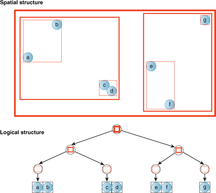
Figure 37.12: A depiction of a 2D axis-aligned box bounding volume hierarchy (BVH). This is an alternate form of tree to the binary space partition tree that provides tighter bounds but does not allow updates without modifying the tree structure.
Unlike a BSP tree, this type of tree provides tight bounds for clusters of primitives and has finite volume. BVHs are commonly built by constructing a BSP tree, and then recursively, from the leaves back to the root, constructing the bounding volumes. The bounding volumes of sibling nodes often overlap under this scheme; as with a BSP tree one can also create a BVH that splits primitives to maintain disjoint sibling spaces.
Listing 37.15: Bounding volume hierarchy using axis-aligned boxes.
1 template< class Value, class Trait = PrimitiveKeyTrait<Value> >
2 class BoxBVH {
3 class Node {
4 public:
5 std::vector<Node*> childArray;
6
7 /* Children in this leaf node. These are pointers because a value
8 may appear in two different nodes. */
9 List<Value*> valueArray;
10
11 AABox bounds;
12 };
13
14 Node* root;
15 ...
16 };
The bounding volumes chosen tend to be balls or axis-aligned boxes because those admit compact storage and intersection queries. These are also known as sphere trees or AABB trees, respectively.
37.7. Grid
37.7.1. Construction
A grid is the generalization of a radix-based 1D array. It divides a finite rectangular region of space into equal-sized grid cells or buckets (see Figure 37.13). Any point P within the extent of the grid lies in exactly one cell. The multidimensional index of that cell is given by subtracting the minimal vertex of the grid from P, dividing by the extent of one cell, and then rounding down. For a grid with the minimal corner at the origin and cells of extent one distance unit in each dimension, this is simply the “floor” of the point. Thus, if we hold cell extent constant, the containing cell can be found in constant time, but the storage space for the structure will be proportional to the sum of the number of members and the volume of the grid. Intersection queries on a grid generally run in time proportional to the volume of the query shape (or length, for a ray).
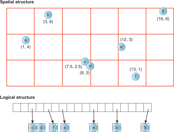
Figure 37.13: A depiction of a 2D grid of values with point keys. The logical structure is that of an implementation that unrolls the underlying 2D array in row-major order starting from the bottom row.
Grids are simple and efficient to construct compared to trees, and insertion and removal incur comparatively little memory allocation or copying overhead. They are thus well suited to dynamic data and are frequently used for collision detection and other nearest-neighbor queries on dynamic objects.
Listing 37.16 shows one possible representation of a grid in three dimensions, with some auxiliary methods. The underlying representation is a multidimensional array. As for images, which are 2D arrays of pixels, grids are frequently implemented by unrolling along each axis in turn to form a 1D array. In the listing, the cellIndex method maps points to 3D indices and the cell method returns a reference to the cell given by a 3D index in constant time.
Listing 37.16: Sample implementation of a 3D x-major grid and some helper functions.
1 struct Index3 {
2 int x, y, z;
3 };
4
5 template< class Value, class Bounds = PrimitiveKeyTrait<Value> >
6 class Grid3D {
7 /* In length units, such as meters. */
8 float cellSize;
9 Index3 numCells;
10
11 typedef List<Value, Bounds> Cell;
12
13 /* There are numCells.x * numCells.y * numCells.z cells. */
14 std::vector<Cell> cellArray;
15
16 /* Map the 1D array to a 3D array. (x,y,z) is a 3D index. */
17 Cell& cell(const Index3& i) {
18 return cellArray[i.x + numCells.x * (i.y + numCells.y * z)];
19 }
20
21 Index3 cellIndex(const Point3& P) const {
22 return Index3(floor(P.x / cellSize),
23 floor(P.y / cellSize),
24 floor(P.z / cellSize));
25 }
26
27 bool inBounds(const Index3& i) const {
28 return
29 (i.x >= 0) && (i.x < numCells.x) &&
30 (i.y >= 0) && (i.y < numCells.y) &&
31 (i.z >= 0) && (i.z < numCells.z);
32 }
33
34 ...
35 };
Since the number of operations involved in finding a grid cell is relatively small, each operation takes a large percentage of the cell dereference time and it is worth micro-optimizing them from the straightforward version shown here. If cellSize is 1.0, the divisions in cellIndex can be completely eliminated. Where that is not possible, multiplying P by a precomputed 1/cellSize value is faster on many architectures than performing the division operations. The floor operation is a relatively expensive floating-point operation that can be replaced with an intrinsic-supported truncate-and-cast-to-integer operation. When numCells.x and numCells.y are powers of two, the multiplications in the cell method become faster bit-shift operations. Finally, at the loss of some abstraction, it is sometimes worth exposing the 1D indexing scheme outside of the data structure. Callers can then iterate directly through the 1D array in steps chosen to walk along any given dimension.
By convention, elements in the 1D array varying along the lowest-indexed dimension (e.g., x) are the ones placed at adjacent memory addresses. When the iteration order is expected to favor some other axis, arranging to unroll along that axis first can yield increased cache coherence. For example, if an application is expected to trace many rays vertically, then making the vertical axis coherent is a good choice.
Sometimes the dominant ray iteration direction cannot be predicted, or iteration will be across multiple dimensions for volume queries such as ball intersection. If memory coherence is a concern for such applications, unrolling the multidimensional array along a space-filling curve can be a good solution. Curves such as the Hilbert [Hil91, Voo91] or Morton [Mor66] (a.k.a. “Z,” for its shape) curves define an indexing scheme that, on average, assign spatially local elements to spatially local memory addresses. These can typically be implemented with a few bitwise operations per index computation.
Tuning the extent of each cell, or equivalently, the number of cells for a given grid extent, requires a good understanding of the kinds of queries that will be performed and the spatial distribution of the data. This issue is best discussed after the query algorithms, so we set it aside until Section 37.7.3.
The inBounds method is convenient for identifying legal indices, which is necessary because the grid has finite extent. For some applications data sets have inherent spatial bounds. For example, in a virtual environment like a video game level with a well-defined boundary, objects will never move beyond the boundary. In this case the finite nature of the grid presents no limitation. In other cases, a scene is known to be very dense in a specific region but contains a few elements that lie far from that region, possibly without any practical spatial bound. In this situation one can extend the grid with a single additional list of elements that lie outside the grid proper. This allows the data structure to represent unbounded extent yet still provide efficient queries within the dense region. If a data set is neither spatially bounded nor primarily clustered in a dense region, the simple grid is likely a poor choice of data structure. However, the sparse hash grid described later in this section may still be appropriate.
37.7.2. Ray Intersection
To find the first intersection of a ray with the primitives in a grid, the query algorithm must walk through the cells of the grid in the order in which the ray enters them, as shown in Figure 37.14. In 2D, this is equivalent to the problem of (ordered) conservative rasterization of the line: Find all cells that touch any part of the line. In 3D, the process is called conservative voxelization.
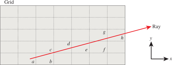
Figure 37.14: Ray traversal of a 2D grid (from [AW87]). To correctly traverse the grid, a traversal algorithm must visit cells a, b, c, d, e, f, g, and h in that order. (Reprinted from Eurographics 1987: Conference Proceedings, 1987 (ISBN 0444702911), Marechal ed., John Amanatides and Andrew Woo, pp. 1–10, “A Fast Voxel Traversal Algorithm for Ray Tracing,” Figure 1.)
Listings 37.17–37.19 give an algorithm for conservative voxelization first proposed by Amanatides and Woo [AW87]. During initialization (Listing 37.17), this algorithm finds the grid cell containing the ray origin. It then computes several vector quantities describing the relative rate of motion of a point Q(t) = P + ![]() t on the ray with origin P and direction
t on the ray with origin P and direction ![]() . From these it can iteratively march through the grid by stepping to the nearest grid line (Listing 37.19).
. From these it can iteratively march through the grid by stepping to the nearest grid line (Listing 37.19).
Listing 37.17: Interface for a 3D grid iterator.
1 class RayGridIterator {
2 public:
3 /* Current grid cell */
4 Index3 index;
5
6 /* Sign of the direction that the ray moves along each axis; +/-1 or 0 */
7 Index3 step;
8
9 /* Size of one cell in units of t along each axis. */
10 Vector3 tDelta;
11
12 /* Distance along the ray of the first intersection with the
13 current cell (i.e., that given by index). Initially zero. */
14 float tEnter;
15
16 /* Distance along the ray to the intersection with the next grid
17 cell. tEnter and tExit can be used to bracket ray ray-primitive
18 intersection tests within a cell. */
19 Vector3 tExit;
20
21 RayGridIterator(const Ray& ray, float cellSize);
22
23 /* Increment the iterator, stepping exactly one cell along exactly one axis */
24 RayGridIterator& operator++();
25 };
Listing 37.18: Initialization of a ray-grid iterator.
1 RayGridIterator::RayGridIterator(const Ray& ray, float cellSize) {
2 tEnter = 0.0f;
3
4 // Iterate over axes, treating points and vectors as linear algebra vectors
5 for (int a = 0; a < 3; ++a) {
6 index[a] = floor(ray.origin()[a] / cellSize);
7 tDelta[a] = cellSize / ray.direction()[a];
8
9 step[a] = sign(ray.direction()[a]);
10
11 float d = ray.origin()[a] - index[a]* cellSize;
12 if (step[a] > 0)
13 // Measure from the other edge
14 d = cellSize - d;
15
16 if (ray.direction()[a] != 0)
17 tExit[a] = d / ray.direction[a];
18 else
19 // Ray is parallel to this partition axis.
20 // Avoid dividing by zero, which could be NaN if d == 0
21 tExit[a] = INFINITY;
22 }
23 }
Listing 37.19: Amanatides and Woo’s algorithm for iterating over the 3D grid cells along a ray, in order.
1 RayGridIterator& operator++() {
2 tEnter = tExit;
3
4 // Find the axis of the closest partition along the ray
5 int axis = 0;
6 if (tExit.x < tExit.y)
7 if (tExit.x < tExit.z)
8 axis = 0;
9 else
10 axis = 2;
11 else if (tExit.y < tExit.z)
12 axis = 1;
13 else
14 axis = 2;
15
16 index[axis] += step[axis];
17 tExit[axis] += tDelta[axis];
18
19 return *this;
20 }
A limitation of this algorithm is that all of the t-based quantities are stored in floating point and incremented by addition. They will thus accumulate the roundoff error. If implemented in fixed-point arithmetic, the error in the intersection positions never increases, but the error in the approximation of the ray direction increases.
For points reasonably near the origin (e.g., with floating-point values less than 104) this algorithm is generally considered sufficiently robust for rendering. However, it may not be sufficiently robust for dynamics simulation, where a missed collision can result in objects becoming stuck or falling through the world.
Listing 37.20 gives the actual intersection algorithm for the grid, considering both primitives and cells. It iterates through all cells that are in bounds and along the ray. For each cell encountered, it uses the underlying list’s intersection method to find the first (if any) intersection.
Listing 37.20: Ray intersection using a 3D grid and iterator.
1 class Grid3D {
2 ...
3
4 /* Assumes that the ray begins within the grid */
5 bool firstRayIntersection(const Ray& ray, Value*& value, float& distance) const {
6
7 for (RayGridIterator it(ray, cellSize); inBounds(it.index); ++it) {
8 // Search for an intersection within this grid cell
9 const Cell& c = cell(it.index);
10 float maxdistance = min(distance, t.tExit);
11 if (c.firstRayIntersection(ray, value, maxdistance)) {
12 distance = maxdistance;
13 return true;
14 }
15 }
16
17 // Left the grid without ever finding an intersection
18 return false;
19 }
20 };
Because primitives may appear in more than one grid cell, it is essential to test only for intersections that occur before the end of the cell at each iteration. An example of a case that depends on this is shown in Figure 37.15. In that figure, consider the intersection test that occurs when the iterator is at the cell labeled b. Because the cells covered by object Y include cell b, during this iteration Y will be tested against the ray. There is in fact an intersection—yet it occurs in cell c, not cell b. Were the algorithm to return that intersection, it would miss the true first intersection, which occurs with object X in cell c.
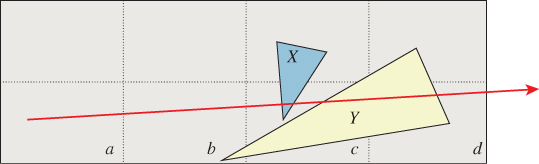
Figure 37.15: A case where it is essential only to test for intersections that lie within each cell during the ray-marching process of ray-triangle intersection accelerated by a spatial grid. (Redrawn from Eurographics 1987: Conference Proceedings, 1987 [ISBN 0444702911], Marechal ed., John Amanatides and Andrew Woo, pp. 1–10, “A Fast Voxel Traversal Algorithm for Ray Tracing,” Figure 1.)
Intuition indicates that the algorithm will run in time proportional to the number of grid cells traversed, because that is the cost of the iterator. The constant overhead of each iteration is very low—a handful of floating-point operations—so the algorithm is practical for cases where we don’t expect the ray to travel too far before striking something. A grid with g subdivisions along k dimensions contains O(gk) cells. The longest ray traversal is the O(g)-length diagonal of the grid. For a grid containing n primitives, in the worst case all of those primitives cover every grid cell along the diagonal but the ray intersects none of them. The intersection query cost is thus O(g · n).
Of course, for such a scene the grid is a poor choice of data structure, since even a spatial list beats its performance. So the worst-case bound is very different from the expected behavior. The grid is better suited to a scene containing roughly uniformly distributed primitives that tend to fit within a grid cell. Likewise, it is better suited to cases of the anticipated ray queries that will progress a small fraction of the scene before striking a primitive.
Trees will exhibit better asymptotic performance under queries than will grids for large scenes with uneven spatial distributions—we expect to see some kind of logarithmic versus linear behavior comparing these data structures in the long run. However, the iteration through empty cells in a grid is fairly fast. Thus, the constant applied to the linear (in the length of the array) time cost term is small and one can afford to traverse many cells for each ray. For scenes of bounded size, the grid may outperform the tree on ray-intersection queries, especially if the time to build the data structure is factored into the net runtime.
37.7.3. Selecting Grid Resolution
If we expect to perform many box or ball intersections, then we should size the grid based on the expected intersection object size so that the intersection algorithm will typically have to examine only a small number of cells (maybe one to four).
Ray intersection on a grid takes time linear in the length of the ray because the number of grid cells to examine is asymptotically proportional to the length of the ray. It also takes time linear in the number of primitives in the grid cells that are encountered. This creates a tension between minimizing the number of grid-intersection tests and the number of element-intersection tests. We assume that grid-intersection tests are less expensive than element intersections. The cost ratio for each kind of test is probably constant, but it may vary over a large range—say, 3:1 for ray-sphere : ray-grid time and 200:1 for ray-implicit-surface : ray-grid time. We might have millions of each kind of potential intersection with significantly varying probability of occurrence. Moreover, changing that ratio affects the space cost of the data structure, which impacts both viability and memory performance. So it is not obvious which kind of intersection test the data structure should favor for performance. The answer is that it depends on the structure of the scene as well as the cost of the intersection tests.
We do know that if we make g large, the grid squares are small, as depicted in Figure 37.16 (left). This reduces the number of elements to be tested in each nonempty cell, but it increases the number of cells that we need to examine. That is good for dense scenes. The figure depicts this by highlighting the primitives that are tested against the ray. That is a small fraction of the elements in the grid in the figure, but it is a large number of grid borders compared to the number of elements in the grid.
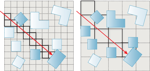
Figure 37.16: (Left) Large g gives small grid cells. A ray iterator must touch many cells (shown with solid black borders), but most of those will be empty. This is good if the cost of testing for a geometric intersection is large compared to the cost of iterating through (or storing) cells. (Right) Small g gives large grid cells. A ray iterates through few grid cells, but those contain many elements: The conservative ray-cell test produces many false positives. This is good if the cost of testing for a geometric intersection is small compared to that of iterating through cells.
If we make g small, the grid squares are large. This allows the ray to quickly step through large volumes of empty space, but it increases the number of elements that must be tested in each nonempty cell encountered. That is good for sparse scenes. Figure 37.16 (right) shows a coarse grid over the same scene from Figure 37.16 (left). For the coarse grid, there are relatively few ray-grid intersections, but many more ray-element intersection tests must be performed within each grid cell.
We describe scenes that contain a mixture of dense and sparse areas as having a nonuniform spatial distribution of elements. A grid is likely a poor data structure for ray intersection in a scene of nonuniform density because no single g constant can serve both areas well. A tree is a better choice in that case because it can adapt to varying spatial density.
There are three layers of subtlety that can subvert this conclusion. At first, it seems that a grid will rarely be a useful data structure. That is because many graphics scenes represent only surface geometry. This makes their spatial distribution of geometry inherently nonuniform, in the sense that the primitives cluster at the surfaces of objects and not on their interior.
The second point is that this characterization itself depends on scale, so it is not a safe generalization. The Manhattan area of New York City comprises tall buildings on a mostly regular grid. Figure 37.17 shows an idealized top view of such a layout. If we examined a computer graphics model of the building exteriors over a volume about the size of a single room (e.g., choosing g so that g3/n ≈ 4 × 4 × 2.5 m3), we’d find that the geometry is indeed distributed in a nonuniform fashion. That’s because a room volume overlapping the edge of a building would contain geometry, but one on the interior or completely outside the building would be empty.
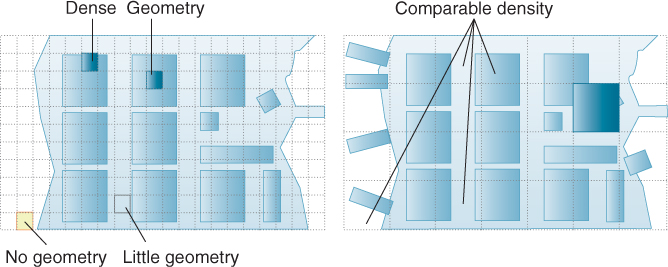
Figure 37.17: Hypothetical top view of a city on an island. (Left) Small grid cells give inhomogeneous geometric density. (Right) Sufficiently large cells produce approximately uniform density for this scene.
If we instead chose grid cells to have at least the footprint of a city block, we’d find that every cell contains about the same number of building exteriors, so the density is nearly uniform. (Of course, some buildings might have more detail in the model than others—let’s just work with a consistent tessellation level.) So part of the challenge in choosing the grid size is that the density, which affects our choice, depends on the grid size itself.
The third point is that constant factors can cause orders of magnitude in performance difference in ray-intersection times with a tree and a grid’s own subdivisions (separate from the cost of intersecting the elements within them). That is because the regular structure of the grid allows efficient memory packing and eliminates the need to explicitly store the grid’s geometry. Where a bounding volume hierarchy must explicitly encode each bounding box, the geometry of each grid cell is implicit in the grid size and requires no memory access to obtain. The process of tracing a ray through a grid is equivalent to the problem of conservatively rasterizing a line. Line rasterization algorithms tend to simplify down to one or two branches and a few additions per pixel (grid cell) on the line’s (ray’s) path. If the ray-grid cell intersection is 50x faster than the ray-tree-node intersection, we can afford to look at many empty grid cells before the inefficiency of doing so overwhelms the performance advantage.
37.8. Discussion and Further Reading
We’ve covered a lot of ground in this chapter at a bunch of different levels of detail and abstraction. Now let’s step back and review the big picture. Relatively straightforward application of basic computer science principles to spatial data structures for representing a scene can return huge speedups for rendering and collision detection. Of course, there are a lot of caveats about avoiding degenerate cases and optimizing for peak performance. But you’d be crazy not to use these kinds of structures, because no constant speedup could possibly make a program scale to large scenes as well as even the simplest spatial tree.
Common sense, backed by examples of some specific cases, led us to the following big observations.
1. Different data structures work well in different places, and the choice isn’t always determined by their asymptotic behavior. Sometimes testing in practice is the best solution.
2. Even when you’ve found the best data structure, you may need to do some tuning.
3. Hardware tricks can sometimes buy you another factor of ten or more.
These items are shown in order: You should choose the right data structure before you try to do hardware-based optimizations; you should test on sample scenes before you do your data-structure tuning.
Spatial data structures continue to be a hot topic in computer graphics. You should experiment by nesting (e.g., Grid3D< BSPTree<Triangle> >) and combine elements of different structures. It is quite common to outperform results from the literature that use more generic structures if your particular application has not been well researched; that is a large part of how the field moves forward. In any given year there will be several new papers on strategies for placing the partitions in a spatial tree or clustering for BVHs. For example, in 1987, one good idea was to build a ray-primitive intersection structure that took the ray’s direction into account [AK87]; in 2000, Havran’s work on modified surface area heuristics [Hav00] influenced the way that engineers optimized tree builds based on area; in 2010 Pantaleone and Luebke [PL10] targeted massively parallel real-time tree building and tuned for tree build time rather than absolute query time.
It is also common to store the same scene data in more than one structure. For example, you may want a list of characters in the world for efficient iteration during Artificial Intelligence simulation, a hash grid for collision detection, and a BSP tree for rendering them. Often a single complex data structure will contain multiple, simpler data structures. This presents a unified interface but allows it to combine the efficiency for different methods from different single data structures. This approach gains performance at the cost of storage space and implementation complexity. In particular, storing the same data multiple times creates potential for the duplicate state becoming desynchronized, and that must be weighed carefully against the performance advantages.
There are commonly employed data structures and increasingly exotic ones. For example, most nongraphics programs rely on a small number of classic data structures such as arrays, hash tables, and an occasional tree. Most graphics programs rely on those plus the spatial data structures presented in this chapter (with the list and BVH perhaps currently the most popular). There’s a lot of practical wisdom in primarily relying on such a small set of workhorses. It amortizes the cost of polishing and optimizing those structures, and lets the programmer using them focus on his or her application instead of learning about a new interface.
But sometimes a more exotic classic data structure is really needed. For example, if your entire program’s performance depends on having a fast priority queue for a large data set, then it may be time to read a paper about left-leaning red-black trees [Sed] and implementing one. But if your program depends heavily on ray-heightfield intersection performance, then it may be worth investing in a data structure optimized for that case, such as Musgrave’s and Amanatides’s and Woo’s grid-tracing algorithms [MKM89, AW87]. Ray-intersection data structures are a constant topic in the global illumination literature. The ray-tracing state of the art “STAR” reports are a good place to find surveys of current thought (e.g., [WMG+09]). Sphere, box and other primitive intersections often arise in the physical simulation community. The design and analysis issues presented in this chapter apply equally well to the structures already discussed and to new data structures that you will invent on your own.
We’ve used ray-triangle intersection as a motivating example throughout this chapter, in part because ray casting is a common operation in most renderers, and triangle meshes are a preferred representation for most scene geometries. But in the future (and in some contexts even today), both of these may change. It may be, for instance, that tracing frusta (essentially bundles of rays) becomes essential, or that geometry is represented primarily by points, or by spline surfaces, or by some yet-unimagined new kind of primitive. When that happens, the choices of acceleration structures will change as well, but the kinds of analysis we’ve described in this chapter will persist: Tradeoffs involving memory coherence, patterns of access, questions of whether our typical problem is of a size large enough that asymptotic analysis is informative, and the costs of implementation versus use will still guide the choices you make as you compare new structures.