
Chapter 6. Introduction to Fixed-Function 3D Graphics and Hierarchical Modeling
6.1. Introduction
You’ve been introduced to how a 3D scene is projected to 2D to produce a rendered image, and you know the basic facts (substantially clarified in later chapters) about light, reflectance, sensors, and displays. The other required ingredient for an understanding of graphics is mathematics. We’ve found that students understand mathematics better when they encounter it experimentally (as we saw with the order-of-transformations issue in Chapter 2). But performing experiments using 3D graphics requires either that you build your own graphics system, for which the preliminary mathematics is critical, or that you use something premade. WPF is a good example of the latter, providing an easy-to-use foundation for 3D experimentation.
In this chapter, you learn how to use WPF’s 3D features (which we’ll refer to as WPF 3D) to specify a 3D scene, configure lighting of the scene, and use a camera to produce a rendered image. WPF’s classic fixed-function model of light and reflectance is not based on physics directly, and does not produce images of the quality needed for entertainment products like animated films; however, because of the enormous adaptability of the human visual system, it does make pictures that our minds perceive as a 3D scene. The fixed-function model also has the advantage of being widely used in other graphics libraries; it’s a model that researchers in graphics should know due to its extensive use in early graphics research and commercial practice, even though it’s being rapidly superseded. The desire to produce more realistic pictures motivates the extensive discussions of light, materials, and reflectance found throughout the remainder of this book.
6.1.1. The Design of WPF 3D
There are dozens of commonly used 3D graphics platforms, covering a wide variety of design goals. Some are focused on image quality/realism regardless of cost (e.g., systems used to compute the frames for high-quality 3D animated films), while others target real-time interactivity with more-or-less realistic simulation of physical properties (e.g., systems used for creating 3D virtual-reality environments or video games), and yet others make compromises on image quality in order to achieve reasonably fast performance across a wide variety of hardware platforms.
As described in Chapter 2, WPF is a retained-mode (RM) platform—the application uses XAML and/or the WPF .NET API to specify and maintain a hierarchical scene graph stored in the platform. (You’ll learn in Section 6.6.4 why it’s called a “graph”; for now, just think of it as a scene database.) The platform, in conjunction with the GPU, automatically keeps the rendered image in sync with the scene graph. This kind of platform is significantly different from immediate-mode platforms such as OpenGL or Direct3D, which do not offer any editable scene retention. For a comparison of these two different architectures in the context of 3D platforms, see Chapter 16.
WPF’s primary goal is to bring 3D into the domain of interactive user interfaces, and as such it was designed to meet these requirements:
• Support a large variety of hardware platforms
• Support dynamics for low-complexity scenes with a real-time level of performance on hardware that meets basic requirements
• And provide an approximation of illumination and reflection sufficiently efficient for real-time creation of visually acceptable 3D scenes
Here we use WPF 3D to introduce some 3D modeling and lighting techniques by example, taking advantage of WPF’s easily editable scene descriptions to give you a hands-on understanding.
6.1.2. Approximating the Physics of the Interaction of Light with Objects
Each object in a 3D scene reflects a certain portion of incident light, based on the reflection characteristics of the object’s material composition. Moreover, each point on the surface of an object receives light both directly from light sources (those that are not blocked by other objects) and indirectly by light reflected from other objects in the scene. The complex physics-based algorithms that directly model the intrinsically recursive nature of interobject reflection (described in Chapters 29 through 32) require lots of processing; if real-time performance is the goal, they often require more processing power than today’s commodity hardware can provide. Thus, real-time computer graphics is currently dominated by approximation techniques that range from loosely physics-based to eye-fooling “tricks” that are not based on physical laws in any way.
The approximation techniques that generate the highest level of realism demand the most computation. Thus, interactive game applications (for which animating at a high number of frames per second is essential for success) must rely on the fast algorithms that compromise on realism. On the other hand, movie production applications have the luxury of being able to devote hours to computing a single frame of animation.
Many classic approximation algorithms were developed decades ago, when the power of computing and graphics hardware was a tiny fraction of what is available today, to meet two key goals: minimizing processing and storage requirements, and maximizing parallelism (especially in GPUs). These algorithms had their roots in software implementations that began in the late 1960s, grew in generality through the 1970s and 1980s, and were then implemented in increasingly more powerful commercial GPU hardware starting in the 1990s.
A particular sequence of the most successful of these algorithms, commonly called the fixed-function 3D graphics pipeline, has been in use for three decades and was dominant in GPU design until the late 1990s. This pipeline renders triangular meshes, approximating both polyhedral objects and curved surfaces, using simple surface lighting equations (for calculating reflected intensity at triangle vertices, as described in Sections 6.2.2 and 6.5) and shading rules (for estimating reflected intensity at interior points, as described in Sections 6.3.1 and 6.3.2). An application uses the fixed-function pipeline via software APIs of the type found in classic commodity 3D packages such as earlier versions of OpenGL and Direct3D. WPF is one of the newer APIs providing a fixed-function pipeline, and as we present its basic feature set throughout the rest of this chapter, we will provide a brief introduction to the classic approximation techniques, how well they “fool the eye,” and what their limitations are.
Although the fixed-function pipeline is an excellent way to start experimenting with the use of 3D graphics platforms (thus our choice of WPF here), it is no longer de rigueur in modern graphics applications, for which the programmable pipeline (introduced in Sections 16.1.1 and 16.3) is now the workhorse. As GPU technology continues its rapid evolution, higher-quality approximations become more feasible in real time, and the ability to simulate the physics of light–object interaction in real time becomes ever more feasible.
6.1.3. High-Level Overview of WPF 3D
WPF’s 3D support is closely integrated with the 2D feature set described in Chapter 2, and is accessed in the same way. XAML can be used to initialize scenes and implement simple animation, and procedural code can be used for interactivity and runtime dynamics. To include a 3D scene in a WPF application, you create an instance of Viewport3D (which acts as a rectangular canvas on which 3D scenes are displayed) and use a layout manager to integrate it into the rest of your application (e.g., alongside any panel of UI controls).
A Viewport3D is similar to a WPF Canvas in that it is blank until given a scene to display. To specify and render a scene, you must create and position a set of geometric objects, specify their appearance attributes, place and configure one or more lights, and place and configure a camera.
The 3D equivalent of the 2D abstract application coordinate system is the world coordinate system, with x-, y-, and z-axes in a right-handed orientation (as explained later in Figure 7.8). The unit of measurement is abstract; the application designer can choose to use a physical unit of measurement (such as millimeter, inch, etc.), or to assign no semantics to the coordinates. The scene’s objects, the camera, and the lights are placed and oriented using world coordinates.
The use of physical units is optional, but can be helpful to accurately emulate some kind of physical reality (e.g., meters for modeling an actual neighborhood’s houses and streets, or millimicrons for modeling molecules). The WPF platform itself is not informed of any semantics the application might attach to the units.
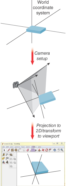
The scene is rendered to the display device via the pipeline represented at a very high level in Figure 6.1. The camera is positioned in the modeled world using world coordinates, and it is configured by specification of several parameters (e.g., field of view) that together describe a view volume—the pyramid-shaped object shown in the middle subfigure. (You’ll learn a great deal about camera specification and view volumes in Chapter 13, and we’ll examine the camera specification from the OpenGL perspective in Chapter 16.) The portion of the scene captured in the view volume is then projected to 2D, resulting in the rendering shown in the viewport, which will appear in the application’s window.
As is the case in WPF 2D, the platform automatically keeps the rendering in sync with the modeled world. For example, making a change to the scene or to the camera’s configuration automatically causes an update to the rendering in the viewport. Thus, animation is performed by editing the scene at runtime, performing actions such as the following:
• Adding or removing objects
• Changing the geometry of an object (e.g., editing its mesh specification)
• Transforming (e.g., scaling, rotating, or translating) objects, the camera, or geometric (in-scene) light sources
• Changing the properties of a material
• Changing the characteristics of the camera or lights
6.2. Introducing Mesh and Lighting Specification
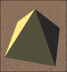
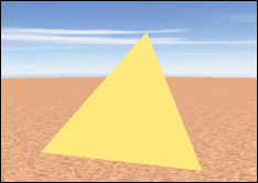
In this section, we will use XAML to build a four-sided, solid-color pyramid, depicted atop a sandy desert floor in Figure 6.2 from the point of view of a lowflying helicopter. In this section, we focus on the construction and lighting of just the pyramid (ignoring the sky and desert floor).
6.2.1. Planning the Scene
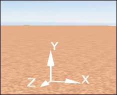
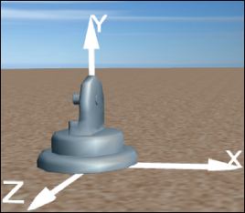
Let’s assume our desert floor is coplanar with the xz ground plane of the right-handed 3D coordinate system, as shown in Figure 6.3. To honor the great Mesoamerican Pyramid of the Sun (75 meters in height) near Mexico City, we’ll give our pyramid that height, with a base of 100 m2. As such, we’ll choose meters as our unit of measurement. We will place our pyramid so that its base is on the xz ground plane, with its center located at the origin (0, 0, 0), its four corners located at (±50, 0, ±50), and its apex located at (0, 75, 0).
6.2.1.1. Preparing a Viewport for Content
To be visible, the viewport must live inside a WPF 2D structure such as a window or a canvas. For this example, we chose to use a WPF Page as the 2D container for the viewport, as it simplifies the use of interpreted development environments such as Kaxaml. Here we create a Page and populate it with a viewport of size 640 × 480 (measured in WPF canvas coordinates, as described in Chapter 2):
1 <Page
2 xmlns="http://schemas.microsoft.com/winfx/2006/xaml/presentation"
3 xmlns:x="http://schemas.microsoft.com/winfx/2006/xaml"
4 >
5 <Page.Resources>
6 Materials and meshes will be specified here.
7 </Page.Resources>
8 <Viewport3D Width="640" Height="480">
9 The entire 3D scene, including camera, lights, model, will be specified here.
10 </Viewport3D>
11 </Page>
Note: Here again, as in Chapter 2, some of XAML’s “syntactic vinegar” will be obvious and may inspire questions. However, this chapter is not intended to be an XAML reference or to replace .NET’s documentation; our focus is on semantics, not syntax.
The camera, the lights, and the scene’s objects are specified inside the Viewport3D tag. The basic template of a viewport and its content looks like this:
1 <Viewport3D ... >
2
3 <Viewport3D.Camera>
4 <PerspectiveCamera described below />
5 </Viewport3D.Camera>
6
7 <!- The ModelVisual3D wraps around the scene’s content ->
8 <ModelVisual3D>
9 <ModelVisual3D.Content>
10 <Model3DGroup>
11 Lights and objects will be specified here.
12 </Model3DGroup>
13 </ModelVisual3D.Content>
14 </ModelVisual3D>
15 </Viewport3D>
We want the camera to be initially placed so that it lies well outside the pyramid, but is close enough to ensure that the pyramid dominates the rendered image. So we will position the camera at (57, 247, 41) and “aim” it toward the pyramid’s center point.1
1. Determining the numeric values that make a scene “look right” is often the result of trial and error; thus, scene design is greatly facilitated by interactive 3D development environments that offer instant feedback while a designer experiments with the placement and orientation of objects, cameras, and lights.
1 <PerspectiveCamera
2 Position="57, 247, 41"
3 LookDirection="-0.2, 0, -0.9"
4 UpDirection="0, 1, 0"
5 NearPlaneDistance="0.02" FarPlaneDistance="1000"
6 FieldOfView="45"
7 />
The camera is a geometric object, placed in the scene’s world coordinate system (via the Position attribute) and oriented via two vectors.
• LookDirection is a vector specifying the direction of the camera projection, in world coordinates. Think of the LookDirection as the center line of the barrel of the lens that you are pointing toward the central object.
• UpDirection rotates the camera about the look-direction vector to specify what will constitute the “up” direction to the viewer. In our example, in which the ground plane is the xz-plane, the up-direction vector [0, 1, 0]T simulates a stationary tripod on the desert sand set up to photograph the pyramid, with the image plane perpendicular to the ground plane.
Additionally, the width of the camera’s field of view can be specified as an angle in degrees; for example, a wide-angle lens can be simulated with a wide field of view such as 160°. Also, two clipping planes can be specified to prevent anomalies that occur when objects are too close to the camera (NearPlaneDistance property), and to reduce computation expense by ignoring objects that are very distant (FarPlaneDistance property) and thus too small to resolve due to perspective foreshortening.
Next we light the scene with nondirectional ambient light that applies a constant amount of illumination on all surfaces regardless of location or orientation. (We’ll supplement this with more realistic lighting later.) Ambient light ensures that each surface is illuminated to some degree, preventing unrealistic pure-black regions on surfaces facing away from light sources. (Such regions would, in the “real world,” be subjected to at least some level of interobject reflection.) The amount of ambient light is kept to a minimum when used in combination with other lighting, but in this initial scene, ambient is the only lighting type, so we’ll use full-intensity white to ensure a bright rendering. We specify this light by adding an AmbientLight element inside the Model3DGroup element:
<AmbientLight Color="white"/>
At this point, we recommend that you start running module #1 (“Modeling Polyhedra...”) of the laboratory software for this chapter, available in the online resources. We will refer to this module throughout this section.
6.2.1.2. Placing the First Triangle
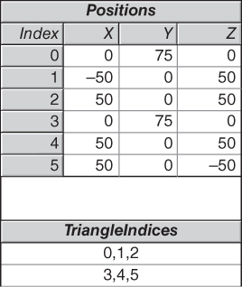
It is no coincidence that we have selected a pyramid as our first example object, since the triangular mesh is the only 3D primitive type currently supported by WPF (and is the most common format generated by interactive modeling applications). The first step in creating a 3D object is to define a resource object of type MeshGeometry3D by providing a list of 3D Positions (vertices) and a list of triangles. The latter is specified via the TriangleIndices property, in which we specify each triangle via a sequence of three integer indices into the zero-based Positions array. In this case, we are specifying a mesh containing just one triangle, the first face of our pyramid. Figure 6.4 shows a tabular representation of the mesh.
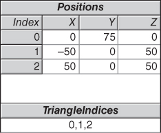
It is the programmer’s responsibility to identify the front side of each triangle, because the front/back distinction is important, as we will soon discover. Thus, when specifying a vertex triplet in the TriangleIndices array, list the vertex indices in a counterclockwise order from the point of view of someone facing the front side. For example, consider how we are presenting the vertices of the single triangle of our current model. In the TriangleIndices array, the three indices into the Positions array are in the order 0, 1, 2. Thus, the vertices are in the sequence (0, 75, 0), (–50, 0, 50), (50, 0, 50), which is a counterclockwise ordering, as shown in Figure 6.5.
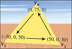
Figure 6.5: Identification of the front side of a mesh triangle via counterclockwise ordering of vertices.
The XAML representation of this mesh is as follows:
1 <MeshGeometry3D x:Key="RSRCmeshPyramid"
2 Positions="0,75,0 -50,0,50 50,0,50"
3 TriangleIndices="0 1 2" />
This mesh specification appears in the resource section of the XAML, and thus is similar to a WPF 2D template resource in that it has no effect until it is used or instantiated. So the next step is to add the 3D object to the viewport’s scene by creating an XAML element of type GeometryModel3D, whose properties include at least the following.
• The geometry specification, which will be a reference to the geometry resource we created above.
• The material specification, which is usually also a reference to a resource. The material describes the light-reflection properties of the surface; WPF’s materials model provides approximations of a variety of material types, as we shall soon see in Section 6.5.
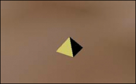
Let’s keep things basic for now, and define a basic solid-yellow material resource, earmarked for the front side of each surface, giving it a unique key for later referencing:
1 <!- Front material uses a solid-yellow brush ->
2 <DiffuseMaterial x:Key="RSRCmaterialFront" Brush="yellow"/>
We now are ready to create the element that will add this single-triangle mesh to our scene. We place this XAML as a child of the Model3DGroup element:
1 <GeometryModel3D
2 Geometry="{StaticResource RSRCmeshPyramid}"
3 Material="{StaticResource RSRCmaterialFront}"/>
Our image of the model now appears as shown in Figure 6.6.
In the lab, select the “Single face” option in the model drop-down list. If you wish, click on the XAML tab to examine the source code generating the scene. Activate the turntable to rotate this triangle around the y-axis.
If we were to rotate this triangular face 180° around the y-axis, to examine its “back side,” we would obtain the puzzling image shown in Figure 6.7.
Figure 6.7: First triangle’s back side, invisible due to lack of specification of a material for the back side.
The triangle disappears due to a rendering optimization: WPF by default does not render the back sides of faces. This behavior is satisfactory for the common case of a “closed” object (such as the pyramid we intend to construct) whose exterior is composed of the front sides of the mesh’s triangles. For such a closed figure, the back sides of the triangles, whose surface normals point toward the object’s interior, are invisible and need not be rendered.
For our current simple model—a lone triangle—it is useful to disable this optimization and show the back face in a contrasting color, by setting the BackMaterial property to refer to a solid-red material that we will add to the resource section with the key RSRCmaterialBack:
1 <GeometryModel3D
2 Geometry="{StaticResource RSRCmeshPyramid}"
3 Material="{StaticResource RSRCmaterialFront}"
4 BackMaterial="{StaticResource RSRCmaterialBack}"/>
As a result, the back face now is visible when the front faces away from the camera, as shown in Figure 6.8.
In the lab, check the box labeled “Use back material” and keep the model spinning.
With the first face of the pyramid now in place, let’s add the second face, using the strategy represented in a tabular form in Figure 6.9. Notice that the vertices shared by the two faces (V0 and V2) have separate entries in the Positions array, effectively being listed redundantly.
1 <MeshGeometry3D x:Key="RSRCmeshPyramid"
2 Positions="0,75,0 -50,0,50 50,0, 50
3 0,75,0 50,0,50 50,0,-50"
4 TriangleIndices="0 1 2 3 4 5" />
The result appears in two snapshots of the spinning model shown in Figure 6.10.
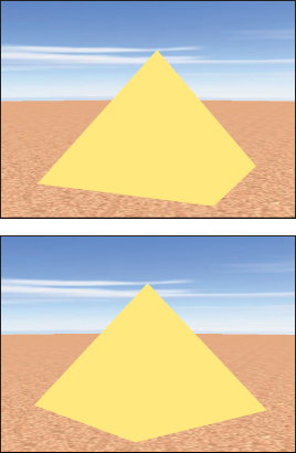
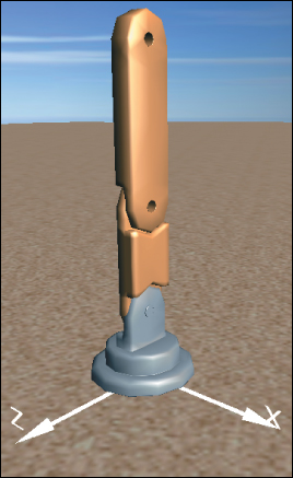
Figure 6.10: Renderings of the partial pyramid in two distinct orientations, in an environment containing only ambient light.
6.2.2. Producing More Realistic Lighting
There is an obvious problem with this rendering: A single constant color value is being applied to both faces of the model, regardless of orientation. But in a daytime desert scene, one would expect variation in the brightness of the pyramid’s faces, with a bright reflection from those facing the sun and lesser reflection from those facing away from the sun.
The use of the artificial construct of nondirectional ambient lighting as the sole light source produces this unrealistic appearance. In the real world, lights are part of the scene and the light energy hitting a point P on a surface has a direction (a vector, represented by the symbol ![]() , from the light source to point P). Moreover, the energy reflected toward the camera from P is not a constant, but instead is based on a number of variables such as the camera’s location, the surface’s orientation at P, the direction
, from the light source to point P). Moreover, the energy reflected toward the camera from P is not a constant, but instead is based on a number of variables such as the camera’s location, the surface’s orientation at P, the direction ![]() , the reflection characteristics of the object’s material, and others. In Section 6.5 we will examine a lighting equation that takes many of these kinds of variables into consideration, but here let’s take a high-level look at one example of a more realistic light source: the point light, which is a geometric light, having a position in the scene and radiating light in all directions equally (as shown in Figure 6.11). A point light’s presence can introduce a great deal of variation into a scene via its infinite set of values for
, the reflection characteristics of the object’s material, and others. In Section 6.5 we will examine a lighting equation that takes many of these kinds of variables into consideration, but here let’s take a high-level look at one example of a more realistic light source: the point light, which is a geometric light, having a position in the scene and radiating light in all directions equally (as shown in Figure 6.11). A point light’s presence can introduce a great deal of variation into a scene via its infinite set of values for ![]() , which ensures that each point on a surface facing the light receives its energy from a unique
, which ensures that each point on a surface facing the light receives its energy from a unique ![]() direction.
direction.
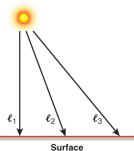
Figure 6.11: Rays emanating from a point light source in the scene, striking points on a planar surface at an infinite variety of angles.
We’ll examine the characteristics and impact of point and other geometric light sources in more detail in Section 6.5, but here let’s start with a simplification: the “degenerate case” of a point light source that is located at an infinite distance from the scene. WPF distinguishes this kind of light source from geometric ones, calling this a directional light. Its rays are parallel (with a constant ![]() , as shown in Figure 6.12), providing an approximation of light from an infinitely distant sun.
, as shown in Figure 6.12), providing an approximation of light from an infinitely distant sun.
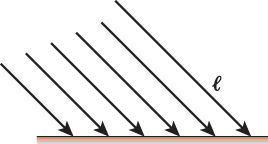
Figure 6.12: Rays emanating from a directional light source, infinitely distant from the planar surface, striking the surface’s points at identical angles.
So, let’s replace the ambient light source with a directional one. We’ll specify its color as full-intensity white, and its direction ![]() as [1, –1, –1]T to simulate the sun’s position being behind the viewer’s left shoulder:
as [1, –1, –1]T to simulate the sun’s position being behind the viewer’s left shoulder:
<DirectionalLight Color="white" Direction="1, -1, -1" />
The direction ![]() for this light (shown as a scene annotation in the lab and in Figure 6.13) is at a 45° angle relative to all three axes, and when projected onto the xz ground plane, it is a vector that travels from the (–x, +z) quadrant to the (+x, – z) quadrant.
for this light (shown as a scene annotation in the lab and in Figure 6.13) is at a 45° angle relative to all three axes, and when projected onto the xz ground plane, it is a vector that travels from the (–x, +z) quadrant to the (+x, – z) quadrant.
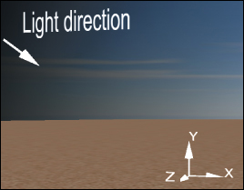
Figure 6.13: Our desert scene’s coordinate system with annotation showing the direction of the rays emanating from the directional light source.
A static 2D image is not the best way to depict 3D information like our light’s ![]() value, so we recommend that you use the lab to follow along with this section’s discussion. Select directional lighting, note the “Light direction” annotation, and use the trackball-like mouse interaction within the viewport to move around in the scene.
value, so we recommend that you use the lab to follow along with this section’s discussion. Select directional lighting, note the “Light direction” annotation, and use the trackball-like mouse interaction within the viewport to move around in the scene.
As introduced in Section 1.13.2, for a completely diffuse surface like that of our pyramid, the light is reflected with equal brightness in all viewer directions and is therefore view-angle-independent. The brightness of the reflected light is only dependent on how directly the incident light hits the surface. Figure 6.14 demonstrates how this directness is measured, by determining the angle θ between ![]() and the surface normal n. The larger the value of θ, the more oblique the light is, and thus the less energy reflected.
and the surface normal n. The larger the value of θ, the more oblique the light is, and thus the less energy reflected.
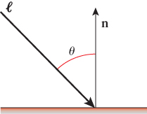
Figure 6.14: The angle θ, defined as the angle between the incoming light direction ray ![]() and the surface normal n.
and the surface normal n.
Given the angle θ and the incident light’s intensity Idir, the reflected intensity is calculated by Lambert’s cosine rule, which was introduced in Section 1.13.2:
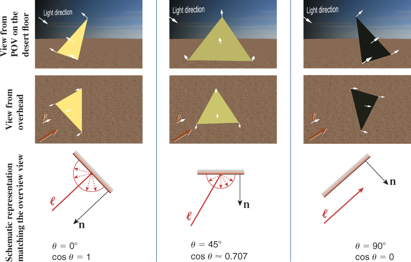
Figure 6.15 demonstrates this equation’s effect on a single-triangle model, for various values of θ achieved by rotating the pyramid on an invisible turntable. In the figure, the length of each dashed red vector depicts the intensity of the reflected energy in its indicated direction, for the given value of θ. With perfectly diffuse reflection, light is reflected with equal intensity in all directions, and therefore, that length is a constant for any given value of θ. The locus of the endpoints of the reflection vectors for all possible reflection angles is thus a perfect hemisphere in the case of diffuse reflection. (In our 2D figure, of course, this envelope appears as a semicircle.)
This equation, being independent of viewing angle, cannot simulate glossy materials such as metals and plastic that exhibit highlights at certain viewing angles. Another oversimplification in the equation is an unrealistic lossless reflection of all incoming light energy when θ = 0°. In reality, some amount of light energy is absorbed by the material and thus is not reflected. Section 6.5 describes a more complete model that corrects these and other problems.
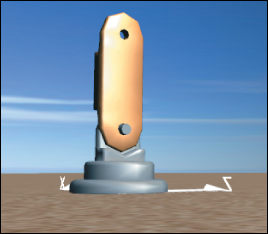
With directional lighting replacing ambient lighting, processed by the Lambert lighting model, the results are more realistic, as you can see in the images in Figures 6.16 and 6.17.
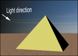
Figure 6.16: Rendering of the pyramid with directional lighting, with θ close to 90° for the rightmost visible face.
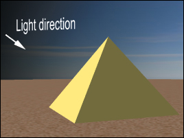
Figure 6.17: Rendering of the pyramid with directional lighting, with θ approximately 70° for the rightmost visible face.
In the lab, activate the directional lighting by selecting “directional, over left shoulder” and enabling turntable rotation. Observe the dynamic nature of the lighting of the yellow front face; it may help to occasionally pause/resume the turntable’s motion. Observe the display of the value of θ and cos θ, and note how the yellow face approaches zero illumination as θ approaches and passes 90°. Select different models and examine the two-face and full four-face models in this new lighting condition.
Lambert’s cosine rule for idealized diffuse reflection has two key characteristics: (1) The reflected intensity is independent of view angle and (2) it depends only on the cosine of the angle between the incoming light direction ![]() and the normal at a point on the surface. To gain an intuitive understanding of these phenomena, find a matte surface such as a clean chalkboard or a painted wall without any sheen, and point a bright light at the surface. Now pick a bright spot on the illuminated area and look at it from a variety of locations through a tube with a diameter so tiny that all you see is a uniformly lit “dot” (simulating what a radiometer would detect). Note that as you move your point of view, the dot’s apparent brightness will remain constant, while it would vary if you performed this same experiment with a shiny surface. Varying the angle of incidence of the light source, however, will cause the reflected brightness to vary with the cosine of the angle. If you are curious about the math behind this rule, consult Section 7.10.6.
and the normal at a point on the surface. To gain an intuitive understanding of these phenomena, find a matte surface such as a clean chalkboard or a painted wall without any sheen, and point a bright light at the surface. Now pick a bright spot on the illuminated area and look at it from a variety of locations through a tube with a diameter so tiny that all you see is a uniformly lit “dot” (simulating what a radiometer would detect). Note that as you move your point of view, the dot’s apparent brightness will remain constant, while it would vary if you performed this same experiment with a shiny surface. Varying the angle of incidence of the light source, however, will cause the reflected brightness to vary with the cosine of the angle. If you are curious about the math behind this rule, consult Section 7.10.6.
6.2.3. “Lighting” versus “Shading” in Fixed-Function Rendering
The Lambert equation presented above, and the more complete equation presented in Section 1.13.1, are examples of functions that compute the amount of light energy that is reflected from a given surface point P toward the specified camera position.
A lighting equation, like the Lambert equation, is an algorithmic representation of the way a surface’s material reflects light. From a theoretical point of view, a renderer processes a given visible surface by “loading” the lighting equation for its material, and “executing” it for points on that surface. (Interestingly, in programmable-pipeline hardware, this abstraction isn’t too far from the truth!) For which surface points should the equation be executed? A reasonable approach is to perform the calculation once for each pixel covered by the surface’s rendered image, executing the equation for a representative surface point for each such pixel. Offline rendering systems use an approach like this, but that strategy is too computationally expensive for real-time rendering systems running on today’s commodity hardware. The approach taken by many such systems—including fixed-function pipelines such as WPF’s, as well as programmable pipelines—is to compute the lighting only at key points on the surface, and to use lower-cost shading rules2 to determine values for surface points lying between the key points.
2. As discussed in Section 27.5.3, this classic use of the term “shading” to refer to efficient determination of lighting at interior points conflicts with modern uses of the terms “shading” and “shader.”
For example, let’s examine the simplest shading technique, known as flat shading or constant shading, in which one vertex of each triangle is selected as the key vertex for that triangle. The lighting equation is executed to compute the illumination value for that vertex, and the entire triangle is filled with a copy of that value. An example rendered image using flat shading is shown in Figure 6.18, in which we’ve highlighted three triangles and the key vertex that was the determinant for each.
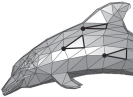
Figure 6.18: Flat-shaded rendering of a dolphin mesh model, with three triangles highlighted to demonstrate the concept of the key vertex.
Flat shading may be appropriate for pyramids, but as Figure 6.18 shows, when the triangular mesh is approximating a curved surface a more sophisticated shading technique is clearly needed. In the next section, we describe a popular real-time shading technique designed to address the problem of rendering curved surfaces.
6.3. Curved-Surface Representation and Rendering
Survey the room around you and you’ll find that most objects have some curved surfaces or rounded edges. A purely faceted polyhedron like our simple pyramid is quite rare in the “real world.” Thus, in most cases, a triangular mesh in a 3D scene is not being used to represent an object exactly, but rather is being used to approximate an object.
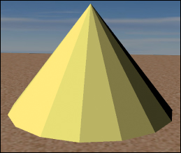
For example, we can approximate a circular cone using a many-sided pyramid. With just 16 faces, flat shading produces a fairly good approximation of a cone (as seen in Figure 6.19), but it doesn’t really “fool the eye” into accepting it as a curved surface.
Increasing the number of facets (e.g., to 64 sides, as shown in Figure 6.20) does help improve the result, but the approximation is still apparent. Attempting to solve the problem merely by increasing the mesh’s resolution is not only expensive (in terms of storage/processing costs) but also ineffective: If the camera’s position is moved toward the mesh, at some point the faceting will become apparent.
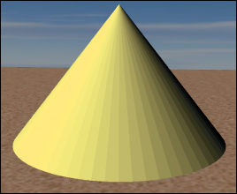
Figure 6.20: Flat-shaded rendering of a cone with 64 sides, reducing (but not eliminating) the obvious faceting.
You might want to visit the “Modeling Curved Surfaces” module of the laboratory to see the effect of changes in the facet count when flat shading is in effect. You can zoom in/out by dragging the mouse (when the cursor is within the viewport) while holding down the right mouse button. Note how increasing the number of facets can only fool the eye at a distance—zooming in exposes the fraud easily. Note also that motion of the object makes the approximation even more obvious, especially at the bottom edge.
6.3.1. Interpolated Shading (Gouraud)
The task of finding an efficient way to produce acceptable images of curved surfaces from low-resolution mesh approximations was particularly urgent in the early days of computer graphics, when computer memory was measured in kilobytes and processors were many orders of magnitude less powerful than they are today. Per-vertex lighting with flat shading was widely used, but there was an obvious need for a shading technique that would fool the eye and allow the rendered image to approximate the curved surface represented by the mesh, even for a low-resolution mesh, at minimal processor and memory cost. In the early 1970s, University of Utah Ph.D. student Henri Gouraud refined a shading technique based on interpolation of intensity values at mesh vertices, using algorithms like those described in the opening sections of Chapter 9. To appreciate the difference in quality between flat shading and Gouraud shading, compare the two renderings of the Utah teapot in Figures 6.21 and 6.22.

Let’s first examine Gouraud interpolation in two dimensions. In Figure 6.23, the curved 2D surface is shown in yellow, the approximation mesh of 2D line segments in black, and the vertices in green. At each vertex, the lighting model (in this case, diffuse Lambert illumination) has computed a color for that vertex. The result of the process of shading (to compute the color across the interior points) is shown for both flat shading and Gouraud interpolated shading.
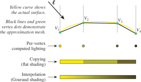
Figure 6.23: Comparison of flat shading and Gouraud shading, two different techniques for determining intensity values between the vertices at which lighting calculations were performed.
As we have seen, the Lambert lighting equation depends on the value of n, the surface normal. Thus, to produce the color value at vertex V, the renderer must determine what we call the vertex normal—that is, the surface normal at the location of V. How should this be determined?
If the curved surface is analytical, for example, a perfect sphere, the equation used to generate the surface can provide the surface normal for any point. However, the approximation mesh itself is often the only information known about the surface’s geometry. This limitation is alleviated by use of Gouraud’s simple strategy for determining the vertex normal via averaging.
In 2D, the vertex normal is computed by averaging the surface normals of the adjacent line segments, as shown in Figure 6.24. For example, the vertex normal for V2 is the average of the surface normals for the line segments ![]() and
and ![]() .
.
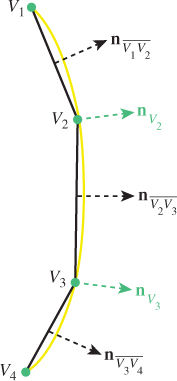
Figure 6.24: Calculating a vertex normal in 2D, as an average of the normals of the two adjacent line segments.
In 3D, the vertex normal is computed by averaging the surface normals of all adjacent triangles, as depicted in Figure 6.25 for a scenario in which four triangles share the vertex.
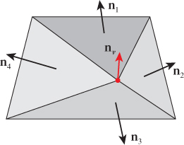
Figure 6.25: Calculating a vertex normal in 3D, as an average of the surface normals of all triangles sharing the vertex.
The success of this technique lies in the fact that, for a mesh that is sufficiently fine-grained, the vertex normal computed via averaging is typically a very good approximation of the surface normal of the actual surface being approximated. (Chapter 25 discusses some limitations of this approximation.) For example, in the 2D representation shown in Figure 6.24, note that ![]() looks like a very good estimate of the normal to the yellow surface at the location of V2. The accuracy of the computed normal is of course dependent on the granularity of the mesh, and the granularity requirement increases in areas of discontinuity.
looks like a very good estimate of the normal to the yellow surface at the location of V2. The accuracy of the computed normal is of course dependent on the granularity of the mesh, and the granularity requirement increases in areas of discontinuity.
We suggest that you return to the curved-surface module of the lab, and select “Gouraud shading.” Note the success of the interpolation even with a minimal number of facets. You will notice that, if the granularity is extremely low (e.g., 4 or 8) and/or the model is rotating, the silhouette of the cone—its bottom edge where it meets the ground—unfortunately continues to exhibit the mesh’s structure, reducing the effectiveness of the “trick.”
6.3.2. Specifying Surfaces to Achieve Faceted and Smooth Effects
WPF’s rendering engine uses Gouraud shading unconditionally; in other words, WPF does not offer a rendering “mode” allowing the application to select between flat shading and smooth shading. Yet, in Section 6.2 we were able to create a pyramid with a faceted appearance, and in Figure 6.21 we showed a WPF-generated flat-shaded depiction of the teapot. How were we able to force WPF to generate a flat look?
Examine Figure 6.9 to review how we specified the first two pyramid faces in Section 6.2. Each shared vertex was placed redundantly in the Positions list to ensure that each was referenced by only one face. This causes the calculation of the vertex normal to involve no averaging, since each vertex is attached to only one triangle. The normal at each vertex will thus match the triangle’s surface normal. Since Gouraud smoothing at edges and vertices is based on the averaging of vertex normals, the use of an unshared vertex effectively disables smoothing at that vertex.
Now, suppose that these two faces are part of a pyramid approximating a circular cone. In this case, we do want smooth shading. So, let’s specify the same two triangular faces, but in the TriangleIndices list, let’s “reuse” the vertex data for the shared apex (V0 in Figure 6.27) and the shared basepoint (V2):
1 <MeshGeometry3D x:Key="RSRCmeshPyramid"
2 Positions="0,75,0 -50,0,50 50,0, 50 50,0,-50"
3 TriangleIndices="0 1 2 0 2 3" />
In this specification (shown in Figure 6.26), vertices V0 and V2 are shared by two triangles, resulting in their vertex normals being computed via the averaging technique. The result is shown in Figure 6.28, with a smoothing of the edge between V0 and V2 being quite apparent.
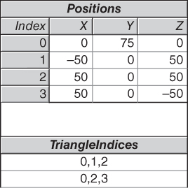
Figure 6.26: Tabular representation of geometric specification of a two-triangle mesh with reuse of shared vertices (the apex and the shared base vertex).
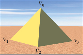
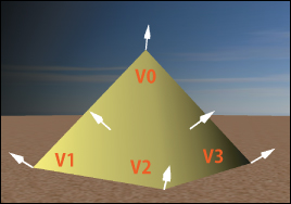
Figure 6.28: Gouraud shaded pyramid, produced in WPF by specifying that the two triangles share vertices V0 and V2, causing their vertex normals to be the average of the surface normals of the two triangles.
In summary, WPF mesh specification requires following a simple rule: You should share vertices that need to participate in Gouraud smoothing, and you should duplicate vertices (i.e., so that each is referenced by only face) that need to be points of discontinuity in the rendered image.
You will find a need for both of these techniques, because typically, complex objects are a hybrid of both smooth curved surfaces and discontinuities where a crease or seam is located and needs to be visible in the rendering. Examples of discontinuities include the location on a teapot where the spout joins the body, and the seam on an airplane where wings join the fuselage. By using vertex sharing appropriately, you can easily represent such hybrid surfaces.
6.4. Surface Texture in WPF
We posit that any computer graphics professional confronted with the question, “What was the single most effective reality-approximation trick in the early history of real-time rendering?” will scarcely skip a beat before exclaiming, “Texture mapping!” When faced with the need to display a “rough” or color-varying material such as gravel, brick, marble, or wood—or to create a background such as a grassy plain or dense forest—it is not advisable to try to create a mesh representing every detail of the fine-grained structure of the material. Consider the complexity of the mesh that would be required to model the dimples and crannies of the rough-hewn stone of an ancient pyramid—our simple four-triangle mesh would balloon into a mesh of millions of triangles, exploding the memory and processing requirements of our application.
Through the “trick” of texture mapping (wrapping a 3D surface with a 2D decal), complex materials (such as linen or asphalt) and complex scenes (such as farmland viewed from an airplane) can be roughly simulated with no increase in mesh complexity. (Chapters 14 and 20 discuss this idea in detail.) For example, the desert sand in our scene was modeled as a square (two adjacent coplanar right triangles) wrapped with the image shown in Figure 6.29.
“Texturing” a 3D surface in WPF corresponds to the act of covering an object with a stretchable sheet of decorated contact paper. Theoretically, we must specify, for each point P on the surface, exactly which point on the paper should touch point P. In practice, however, we specify this mapping only for each vertex on the surface, and interpolation is used to apply the texture to the interior points.
This specification requires a coordinate system for referring to positions within the texture image. By convention, instead of using exact integer pixel coordinates, we refer to points on the image using the floating-point texture coordinate system shown in Figure 6.30, whose axes u and v have values limited to the range 0 to 1.
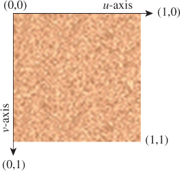
Figure 6.30: Floating-point texture coordinate system applied to the sand-pattern image, with the origin located at the upper-left corner.
In XAML, the first step is to register the image as a diffuse material in the resource dictionary. We have used a solid-color brush previously, but here we create an image brush to define the material:
1 <DiffuseMaterial x:Key="RSRCtextureSand">
2 <DiffuseMaterial.Brush>
3 <ImageBrush ImageSource="sand.gif" />
4 </DiffuseMaterial.Brush>
5 </DiffuseMaterial>
The next step is to register into the resource database the simple two-triangle mesh representing the ground, using the same technique as before, but adding a new attribute to specify the corresponding texture coordinate for each vertex in the Positions array:
1 <MeshGeometry3D x:Key="RSRCdesertFloor"
2 Positions="-9999, 0, -9999
3 9999, 0, -9999
4 9999, 0, 9999
5 -9999, 0, 9999"
6 TextureCoordinates=" 0,0 1,0 1,1 0,1 "
7 TriangleIndices="0 1 3 1 2 3"
8 />
Since this is a mapping from a square (the two coplanar triangles in the 3D model) to a square (the texture image), we declare texture coordinates that are simply the corners of the unit-square texture coordinate system, as shown in Figure 6.31.
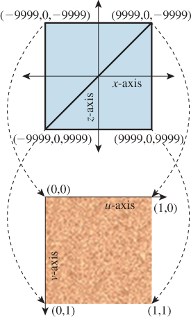
Figure 6.31: Mapping world-coordinate vertices on the two-triangle model of the desert floor to corresponding texture coordinates.
With the material and geometry registered as resources, we are ready to instantiate the desert floor:
1 <GeometryModel3D
2 Geometry="{StaticResource RSRCdesertFloor}"
3 Material="{StaticResource RSRCtextureSand}"/>
The result is shown in Figure 6.32, from a point of view high above the pyramid. The result is not acceptable; there is some subtle variation in the color of the desert floor, but the color patches are huge (in comparison with the pyramid).
The problem is that our tiny 64 × 64-pixel sand decal (which was designed to represent about one square inch of a sandy floor) has been stretched to cover the entire desert floor. The result looks nothing like sand even though our decal provides fairly good realism when viewed unscaled.
Our failure to simulate desert sand here is a case of a reasonable texture image being applied to the model incorrectly. Implementing texturing in WPF requires choosing between two mapping strategies: tiling and stretching.
6.4.1. Texturing via Tiling
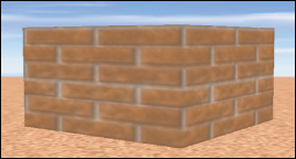
If the texture is being used to simulate a material with a consistent look and no obvious points of discontinuity (e.g., sand, asphalt, brick), the texture image is replicated as needed to cover the target surface. In this case, the texture is typically a small sample image (either synthetic or photographic) of the material, which has been designed especially to ensure that adjacent tiles fit together seamlessly. As an example, consider the texture image of Figure 6.33 showing six rows of red brick.
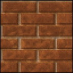
Applying it to each face of a rectangular prism without tiling produces a decent image (Figure 6.34) but the number of rows is insufficient for representing a tall brick fortress. Tiling allows the number of apparent brick rows to be multiplied, producing an image (Figure 6.35) that is more indicative of a tall fortress.
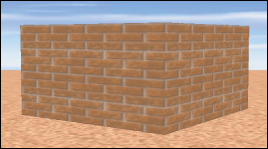
Consult the texture-mapping module of the lab for details on how to enable and configure tile-based texturing in WPF.
6.4.2. Texturing via Stretching
If a texture is being used as a substitute for a highly complex model (e.g., a city as seen from above, or a cloudy sky), the texture image is often quite large (to provide sufficiently high resolution) and may be either photographic or original artwork (e.g., if being used to represent a landscape in a fantasy world). Most importantly, this kind of texture image is a “scene” that would look unnatural if tiled. The correct application of this kind of texture image is to set the mesh’s texture coordinates in such a way as to stretch the texture image to cover the mesh.
For example, in our desert scene, the background sky (as seen often in Figures 6.5 through 6.17) is modeled as a cylinder whose interior surface is stretch-textured with the actual sky photograph shown in Figure 6.36.

Consult the texture-mapping module of the lab for details on how to enable and configure stretch-based texturing in WPF. More information, including algorithms for computing texture coordinates for curved surfaces and a discussion of common texture-mapping problems, is presented in Section 9.5 and in Chapter 20.
6.5. The WPF Reflectance Model
In Section 6.2.2, we presented Lambert’s simple cosine rule for calculating reflected light from a diffuse surface. That simple equation is just one part of the complete WPF reflectance model, which is based on a classic approximation strategy that provides results of acceptable quality, without complex physics-based calculations, on a wide variety of commodity graphics hardware.
6.5.1. Color Specification
The word “color” is used to describe multiple things: the spectral distribution of wavelengths in light, the amount of light of various wavelengths that a surface will reflect, and the perceptual sensation we experience on seeing an object. Representing color precisely is a serious matter to which Chapter 28 is dedicated. Indeed, specifying color via RGB triples—the common approach in graphics APIs and drawing/painting applications—may well be the grossest of all the approximations made in computer graphics practice!
When describing a scene, we specify the colors of the light sources and of the objects themselves. In WPF, specifying the former is straightforward (see Section 6.2.2), but describing the latter is far more complex, requiring the separation of the material into three distinct components. Section 6.5.3 is dedicated to describing this specification technique and the effects it can achieve.
6.5.2. Light Geometry
The two WPF lighting types we have used thus far (ambient and directional) are useful approximations but decidedly unrealistic: They are not considered to be emanating from a specific point in the scene, and their brightness is uniform throughout the entire scene.
A geometric light source adds realism in that it is located in the scene and is attenuated—that is, the amount of energy reaching a particular surface point P is dependent on the distance from P to the light source. WPF offers two geometric light source types.
• A point light emanates energy equally in all directions, simulating a naked bulb suspended from a ceiling without any shade or baffles. Specification parameters include its position and the attenuation type/rate (constant, linear, or quadratic, as described in Section 14.11.9). The lab software for this chapter allows experimentation with this type of light source.
• A spotlight is similar, but it simulates a theatre spotlight in that it spreads light uniformly but restricts it to a cone-shaped volume.
Geometric lights are useful but should still be considered only approximations, since real physical light sources (described in Section 14.11.6) have volume and surface area, and thus do not emit light from a single point.
6.5.3. Reflectance
In our modeling of desert scenes throughout this chapter, we have applied material to our meshes by specifying either a solid color or a texture image. However, there is more to a material than its color. If you’ve shopped for interior-wall paint, you know that you must also choose the finish (flat, eggshell, satin, semigloss), which describes how the painted surface will reflect light.
The physics of how light is reflected from a surface is extremely complex, so for decades, the fixed-function pipeline has relied on a classic approximation strategy called the Phong reflectance (lighting) model that yields an effective simulation of reflection at very little computational cost.3 In the Phong model, a material is described by configuring three distinct components of reflection: ambient (a small constant amount of light, providing a gross simulation of inter-object reflection), diffuse (representing viewer-independent light reflected equally in all directions), and specular4 (providing glossy highlights on shiny surfaces when the viewpoint is close to the reflection ray). The values calculated for the three components—Figure 6.37, (a) through (c)—are summed to produce the final appearance, shown in part (d) of that figure.
3. This non-physics-based reflectance model was invented early in the history of raster graphics and rendering research in the 1970s initially by University of Utah Ph.D. student Bui Tuong Phong and then slightly modified by Blinn, and has been remarkably long-lived, especially in real-time graphics.
4. For this chapter only, we are following the convention that “specular” refers to somewhat concentrated reflections rather than to perfect mirror reflection. Elsewhere specular means “mirrorlike,” while sort-of-specular reflection is called “glossy.” The use of “specular” for glossy follows both Phong’s original paper and the WPF convention, but conflicts with its ordinary meaning of “having the properties of a mirror.”
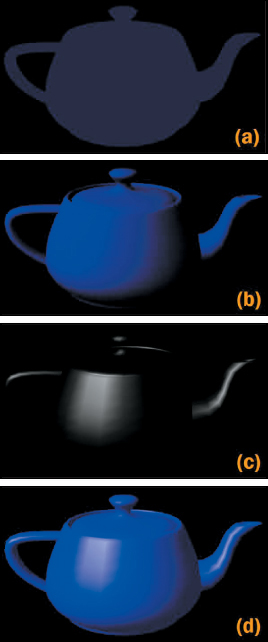
Figure 6.37: Renderings of a teapot, showing the contribution of each of the three components generated by the Phong lighting equation: (a) ambient, (b) diffuse, (c) specular, and (d) result generated by summing the contributions.
The independent nature of the diffuse and specular components allows us to generate the approximate appearance of materials having multiple layers with distinct reflectance characteristics. Consider a polished red apple: On top of its diffuse red layer lies a colorless waxy coating that provides glossy highlights based on the color of the light source (not of the apple). This same pattern of reflection is also very common in plastics, although it is not generated by a multilayer reflectance, but by the nature of the plastic material itself. Our blue plastic teapot (in Figure 6.37) shows this: Its glossy highlights have the colorless hue of the incoming white light, while the diffuse reflections have the blue hue of the plastic. In Section 6.5.3.3 we’ll provide more detail on how to produce this effect. Of course, this simplistic technique of summing noninteracting layers is inadequate for complex materials such as human skin; Section 14.4 presents an introduction to richer, more accurate material models, and Chapter 27 gives full details.
In this section, we describe the lighting equation for WPF’s reflectance model, which is heavily based on, but not completely identical to, the Phong model. Let’s first examine the equation’s inputs that are specified as properties of the material resources (e.g., in WPF elements such as DiffuseMaterial and others enumerated in this chapter’s online materials):
For a solid-color material, the innate colors for the diffuse and specular layers are constant across a surface. For a textured material, the texture image and texture algorithm together determine the diffuse-layer color at each individual surface point.
The three efficiency factors are each expressed as an RGB triple, with each entry being a number between 0 and 1, with 0 meaning “no efficiency” and 1 meaning “full efficiency.” For example, we would specify ka,R = 0.5 for a diffuse layer that reflects exactly half of the red component of the ambient light in the scene.
What we’ve called “reflection efficiency” here is closely related to the physical notion of reflectivity, which we’ll examine in detail in Chapter 26.
Next, let’s examine the inputs that are specified by or derived from the lights that have been placed in the scene, via any of WPF’s light-specification elements, such as DirectionalLight:

A geometic light’s actual contribution is subject to attenuation. The attenuation factor Fatt is calculated for each surface point P, based on the light’s characteristics and distance from P. Thus, the actual light arriving from at the surface point P from the geometric light source is
(FattIgeom,R; FattIgeom,G; FattIgeom,B).
Now that we have enumerated all of the inputs, we are ready to examine the WPF lighting equation. Here is the equation that computes the intensity of the red light that reaches the camera from a specific surface point (we examine each component in detail below):
The sums in the equations above are over all lights of various kinds, which we’ll describe shortly.
If the scene contains multiple lights, and/or if the material uses multiple components (e.g., both ambient and diffuse) with high reflection efficiency coefficients, the computed result may be greater than 100% intensity, which has no meaning since the pixel’s range of red values is limited to the range of 0% to 100% illumination. Simple lighting models simply clamp excessive values to 100%. The “extra” illumination is thus discarded, which can have a negative impact on renderings, including unintended changes in hue or saturation. More sophisticated techniques for dealing with this situation—primarily the use of physical units—are discussed in Chapters 26 and 27. This failure is a consequence of the ill-defined nature of “intensity” that we discussed earlier, and presents a practical and widespread incidence of the failure of the Wise Modeling principle. The model of intensity as a number that varies from 0 to 1 was clearly a bad choice as the scale of scenes and complexity of lighting grew.
As we present the various components of the WPF reflectance model below, you may want to experiment with the effects of the configurable terms by using the lighting/materials laboratory software, and accompanying list of suggested exercises, available in the online resources for this chapter.
6.5.3.1. Ambient Reflection
Ambient light is constant throughout the scene, so the computation of the ambient reflection component is extremely simple and devoid of geometric dependencies. In the WPF reflectance model, there is no ambient innate color, so the material’s diffuse color is used. The red component of the ambient reflection is computed via:
We encourage you to immediately perform the ambient-related experiments suggested in the lighting exercises presented online.
6.5.3.2. Diffuse Reflection
Directional light appears in the diffuse term of the reflectance model, computed by Lambert’s cosine rule described in Section 6.2.2. Here is the red portion of this term, which takes into account all the directional lights in the scene:
The sum here is over all directional lights in the scene. The angle θ will generally be different for each one, as will the intensity Idir,R.
A similar equation sums over the set of geometric light sources, to take into account their attenuation characteristics. This equation is shown as part of the diffuse term in the full equation shown in the table above.
We encourage you to immediately perform the diffuse-related experiments suggested in the lighting exercises presented online.
Note that for solid-color materials, the distinction between the two terms Cd and kd is unnecessary, as far as the math is concerned; you can think of them as a single term. That is, you can fix kd,R at 1.0 and use Cd,R to achieve any effect, and conversely you could fix Cd,R and specify only kd,R. However, the distinction between the two terms is meaningful when the innate color Cd is being provided via texture mapping; in that case, there is a need for a kd,R factor affecting the reflection of the varying color Cd specified by the texture.
6.5.3.3. Specular Reflection
The specular reflectance term is the sum of a computed intensity for each directional and geometric light in the scene. Let’s examine this sum for the directional lights:
Most materials produce a specular reflection that is some mixture of its diffuse color and the light source’s color, but the ratio of the former to the latter varies. You may have noticed that some shiny materials show a specular highlight that is essentially a brighter version of the diffuse color of the material. For example, the shiny highlights on a brass kettle illuminated by a bright light source are a “tinted” version of the light’s color, highly affected by the innate brass color. But, as explained earlier, for plasticlike materials, specular highlights take on primarily the color of the light source rather than of the diffuse color. To achieve this plasticlike appearance, ensure that the product of ks and Cs is a value not biased toward any component color (red, green, or blue) so as to preserve the hue of the incoming light.
This computation also includes a cosine-based attenuation factor, differing from that of Lambert’s law in two ways. First, Lambert’s law compares incoming light to the orientation of the surface alone, and is therefore viewpoint independent. However, specular reflection is highly viewpoint dependent, and thus relies on a different value δ, which in Phong’s original formulation measures the angle between the reflection vector r (computed via the “angle of reflection equals angle of incidence” rule mentioned in Section 1.13.1) and the surface-to-camera vector e, as shown in Figures 6.38 and 6.39. The use of cos δ ensures that the specular effect is strongest when the viewpoint lies on vector r, and weaker as the surface-to-camera vector varies more from vector r.
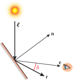
Figure 6.38: Phong’s original technique for computing specular reflection, depicted in a context in which the camera position is very close to the reflection ray.
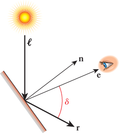
Figure 6.39: Phong’s original technique for computing specular reflection, depicted in a context in which the camera position is not close to the reflection ray. The significant difference in the value of cos δ makes an even greater difference when it’s raised to a large power, so the specular term is nearly zero for this view.
Second, whereas cos δ ensures an intensity drop-off as e varies further from r, we also need to control how “fast” that drop-off is. For a perfect mirror, there is no gradual drop-off; rather, the reflection’s intensity is at a maximum when the viewpoint is directly on vector r, and is zero if not. This binary situation doesn’t occur in real-world materials; instead, there is a large variety in fall-off velocity among different materials. Thus, the equation provides for control of the amount of specularity through the variable s, known as the specular exponent (or specular power) of the material. Values of s for highly shiny surfaces are typically around 100 to 1000, providing a very sharp fall-off. A polished apple, on the other hand, might have an s of about 10, and thus a larger but dimmer area of measurable specular contribution. The lab software lets you experiment with different values of s to become familiar with its effect on specular appearance, and we encourage you to perform the specular-lighting exercises provided in the online material.
6.5.3.4. Emissive Lighting
Many rendering systems additionally offer the artificial notion of self-luminous emissive lighting that allows a surface to “reflect” light that is not actually present externally. Emission is independent of geometry and is not subject to any attenuation. The specification is simply a single color (solid or textured), which is added to the other three components to yield the final intensity value. Note that emission is most useful when emitting a texture—for example, to emulate a nighttime cityscape background or a star-filled sky—but it can also be used to model neon lights that have the particular “look” of a neon tube, although they do not illuminate anything else in the scene. We encourage you to perform the emissive-lighting exercises provided in the online material.
6.6. Hierarchical Modeling Using a Scene Graph
What’s a desert without camels? In this section, we will design a simple articulated robotic camel with some pin joints (highlighted in Figure 6.40) supporting rigid-body rotations on a single axis. This section builds on the modeling and animation techniques you first encountered with the clock example in Chapter 2. While the XAML code examples below are particular to WPF, these techniques for composing and animating complex models are common to all scene-graph platforms.
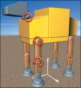
Figure 6.40: WPF’s rendering of the camel constructed via hierarchical modeling, with joints for legs and neck animation.
Throughout this section we will refer you to activities in the “Hierarchical Modeling” module of this chapter’s laboratory. We strongly recommended that you perform the lab activities while reading this section.
6.6.1. Motivation for Modular Modeling
When designing any complex model, a developer should modularize the specification of the geometry by dividing the model into parts that we call subcomponents. There are many reasons for avoiding a monolithic (single-mesh) model.
• Materials are typically specified at the level of the mesh (e.g., the GeometryModel3D element in WPF). Thus, if you want the materials to vary (e.g., to render the camel’s foot using a different material from its shin), you must use subcomponents.
• When a component appears at multiple places in the model (e.g., the camel’s four legs), it is convenient to define it once and then instantiate it as needed. Reusability of components is as fundamental to 3D modeling as it is to software construction, and is a key optimization technique for complex scenes.
• The use of subcomponents facilitates the animation/motion of subparts. If a complex object is defined via a single mesh, movement of subparts requires editing the mesh. But if the design is modular, a simple transformation (of the kind we used in animating the clock in Chapter 2) can be applied to a subcomponent to simulate a motion such as the bending of a knee.
• Pick correlation (the identification of which part of the model is the target of a user’s click/tap action) is more valuable if your model is modularized well. If the user clicks on a single-mesh camel, the result of correlation is simply the identity of the camel as a whole. But if the camel is modularized, the result includes more detail; for example, “the shin of the front-left leg.”
• Editing a single-mesh model is difficult due to interdependencies among the various parts—for example, extending the height of the camel’s legs would, as a side effect, require revising all the vertices in the camel’s head and torso. But when a model is defined using a hierarchy of subparts, the geometry of a subcomponent can be edited in isolation in its own coordinate system, and the assembly process can use transformations to integrate the parts into a unified whole.
These reasons are so compelling that we abstract them into a principle:
![]() The Hierarchical Modeling Principle
The Hierarchical Modeling Principle
Whenever possible, construct models hierarchically. Try to make the modeling hierarchy correspond to a functional hierarchy for ease of animation.
6.6.2. Top-Down Design of Component Hierarchy
One strategy for designing a complex model for animation is to analyze the target object to determine the locations of joints at which movement might be desired. For example, as depicted in Figure 6.40, we might want our camel to have knee and hip joints for leg movements, and a neck joint for head movement.5 The joint locations, along with other requirements such as variations in materials, are then used to determine the necessary component breakdown. Let’s focus first on just the camel’s leg: We need to implement hip and knee joints, and we’d like the option of a distinct material for the foot.
5. Here, our use of the term “joint” is informal and simply identifies locations at which we might want to implement an axis of rotation on a subcomponent to simulate a biological joint or a construction hinge. In sophisticated animation technologies, a joint is far more complex, may support more than one axis, and is often an actual object (distinct from the model’s subcomponents) with structure, appearance, and behaviors derived from principles of physics and biomechanics.
The hierarchy shown in Figure 6.41 fits our needs. In the figure, we distinguish between primitive nodes (meshes with associated materials) and higher-level grouping nodes that combine subordinate grouping nodes and/or primitive nodes. Also, on the lines connecting components, we distinguish between two different types of modeling transformations. As you may recall from Chapter 2, we identify two slightly different uses of modeling transformations.
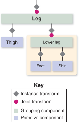
Figure 6.41: Scene graph of the camel-leg model. Here, and below, we use a beige background to highlight a portion of the graph that is being used as a component or submodel.
• An instance transform is used to position, resize, and orient a subcomponent in order to position it properly into a scene or into a higher-level composite object. In our clock application in Chapter 2, we used instance transforms to position the clock hands relative to the clock face, and to reshape a stencil clock hand to form the distinctive shapes of the hour and minute hands. Since the need for proper placement of a subcomponent may be present anytime instantiation is performed, we tend to include an instance transform on each subcomponent in our hierarchical design.
• A joint transform is used to simulate movement at a joint during animation. For example, the knee joint is implemented by a rotation transformation acting on the lower leg, and the hip joint is implemented by a rotation transformation acting on the entire leg. In our clock application, we used this to implement movement of the clock hands.
6.6.3. Bottom-Up Construction and Composition
Now we demonstrate how XAML can be used to construct the model. The order is bottom-up: first generating the primitive components (foot, shin, etc.) and then composing the parts to create the higher-level components.
The activities involved in bottom-up construction are summarized in this table:
6.6.3.1. Defining Geometries of Primitive Components
The design of each primitive component should be an independent task, with its geometry specified in its own coordinate system, as we did for the clock hand in Chapter 2. The abstract coordinate system in which an object is specified is sometimes called the object coordinate system. For convenience, the component should be at a canonical position and orientation—for example, at the origin, centered on one of the coordinate axes, resting on one of the three coordinate planes.
Choosing a physical unit of measurement is optional, but composing the parts is simpler if the dimensions of components are consistent. For example, we have designed the foot as 19 units high (Figure 6.42) and the shin as 30 units high (Figure 6.43) to ensure that composing the two (to form the lower leg) requires only translation of the shin, as shown in Figure 6.45. (We’ll work through the details of the lower leg construction in the next section.) No stretching/compressing (scaling) or rotation actions are necessary. Similarly, the thigh is consistently sized so that the full leg can be built by translating the thigh to connect it to the top of the lower leg.
Note that a typical interactive 3D modeling environment makes it very easy to build canonical, consistent atomic components, via features such as ruler overlays, templates of common volumes, and snap-to-grid editing assistance.
Naturally, if your design incorporates subcomponents obtained from third parties, inconsistencies can be expected, and additional transformations (e.g., resizing or reshaping via scaling) may be required to facilitate composing them with the components you designed. Similar transformation-based adjustments may be necessary when incorporating a completed composite model into an existing scene. For example, if we wish to place our completed camel model (which is well over 100 abstract units in height) into the pyramid scene we constructed previously, we will have to take into account that our scene’s world coordinate system is a physical one with each unit representing 1 meter. Our camel, if placed in that scene without scale adjustment, would be 100 meters tall, towering over our 75-meter pyramid!
6.6.3.2. Instantiating a Primitive Component
Once the primitive components have been designed and their meshes stored in the resource dictionary, each one can be “test-viewed” by instantiating it alone in the viewport, via creation of a GeometryModel3D element. The XAML shown below adds an instance of the foot primitive to our desert-scene viewport:
1 <ModelVisual3D.Content>
2 <Model3DGroup>
3 Lights will be specified here.
4 <GeometryModel3D Geometry="{StaticResource RSRCmeshFoot}"
5 Material=... />
6 </Model3DGroup>
7 </ModelVisual3D.Content>
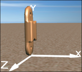
Note that the instantiated foot is not being transformed, so it will appear at the origin of the world coordinate system of the scene, as you can see in Figure 6.42.
Use the Model listbox, along with the turntable feature, to examine the various primitive components of the camel in their canonical positions at their local origins. For example, the shin in its canonical position appears as shown in Figure 6.43.
6.6.3.3. Constructing a Composite Component
A composite node is specified via the instantiation of subcomponents within a Model3DGroup element; the subcomponents are accumulated into the composite node’s own coordinate system.
6.6.3.4. Creating the Lower Leg
Here is a first draft of our camel’s lower leg:
1 <Model3DGroup x:Name="LowerLeg">
2 <GeometryModel3D Geometry="{StaticResource RSRCmeshFoot}"
3 Material=... />
4 <GeometryModel3D Geometry="{StaticResource RSRCmeshShin}"
5 Material=... />
6 </Model3DGroup>
Testing this composite by instantiating it into the viewport yields the rendering shown in Figure 6.44.
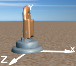
Figure 6.44: Rendering of a first draft of a lower-leg model, constructed by composing the two subcomponents without moving them from their canonical positions at the origin of the coordinate system.
This unsatisfactory result, in which the two models co-inhabit space causing the foot’s ankle region to intersect the shin, occurs because each component is, by design, positioned at the origin of its local coordinate system. When composing parts, we must use instance transforms to properly position the subcomponents relative to one another. Our goal is for the bottom of the shin to be connected to the top (ankle) part of the foot.
Thus, we need to translate the shin in the positive y direction; an offset of 13 units is satisfactory. Note that the foot is already properly positioned for its role in the lower-leg composite and thus needs no transform.
Below is our second draft of the XAML specification for this composite component (with the new lines of code highlighted). A couple of views of the result are shown in Figures 6.45 and 6.46.
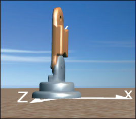
Figure 6.45: Rendering of the lower-leg model, now corrected via application of a modeling transformation on the shin subcomponent.
1 <Model3DGroup x:Name="LowerLeg">
2
3 <GeometryModel3D Geometry="{StaticResource RSRCmeshFoot}"
4 Material=... />
5
6 <GeometryModel3D Geometry="{StaticResource RSRCmeshShin}"
7 Material=... >
8 <GeometryModel3D.Transform>
9 <TranslateTransform3D OffsetY="13"/>
10 </GeometryModel3D.Transform>
11 </GeometryModel3D>@</Model3DGroup>
Return to the lab, and use the hierarchy viewer/editor to add a transform to the shin to repair the lower-leg composite.
6.6.3.5. Creating the Full Leg
Let’s continue our bottom-up implementation by going up to the next level. The “whole leg” is a composition of the lower leg (itself a composite) and the thigh (a primitive). Let’s first compose these two components to form a rigid locked object, and then we’ll attack the challenge of adding a knee joint.
As was the case for the lower leg, one of the subcomponents needs an instance transform (i.e., the thigh needs to be raised 43 units in the y direction) and the other is already at a suitable location. The resultant image is shown in Figure 6.47; the XAML code is as follows:
1 <Model3DGroup x:Name="Leg">
2
3 <!- Build the lower-leg composite (same XAML shown earlier). ->
4 <Model3DGroup x:Name="LowerLeg"> . . . </Model3DGroup>
5
6 <!- Instantiate and transform the thigh. ->
7 <GeometryModel3D Geometry="{StaticResource RSRCmeshThigh}"
8 Material=. . . >
9 <GeometryModel3D.Transform>
10 <TranslateTransform3D OffsetY="43"/>
11 </GeometryModel3D.Transform>
12 </GeometryModel3D>
13
14 </Model3DGroup>
Return to the lab, and select “Thigh” from the list of models to examine that component in isolation. Then select the model “Whole leg”. The undesired merging of the two subcomponents will be obvious. Repair by adding an instance transform to the thigh to translate it on the y-axis. (If you wish, you can jump straight to our solution by choosing “Whole leg auto-composed” from the list of models.)
6.6.3.6. Adding the Knee Joint
The leg is currently locked in a straight position. But, by adding a rotation transformation to the lower leg, we can provide a “hook” that animation logic can use to simulate bending at the knee.
Figure 6.48 shows the leg in its canonical location at the origin, but with a 37° rotation at the knee. (The invisible axis of rotation has been added to this rendered image for clarity.)
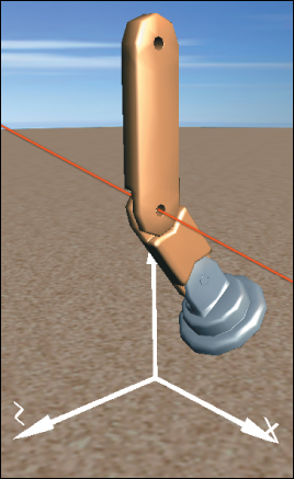
Figure 6.48: Result of specifying a 37° rotation at the knee joint, annotated with a red line through the joint, parallel to the x-axis, showing the axis of rotation.
The WPF element for expressing 3D rotation requires specification of the axis and the rotation amount. The axis is configured via two parameters: an arbitrary directional vector (e.g., [1 0 0]T representing any line that is parallel to the x-axis) and a center point lying on that vector (e.g., the center of the “knee” part of the lower leg, which is (0, 50, 0) in the lower leg’s coordinate system).
Return to the whole-leg model in the lab. Implement the simulated knee joint by adding a rotation transform to the lower-leg component. Set the rotation axis as needed, and then use the numeric spinner to change the rotation amount to produce a knee-bend animation.
The XAML for the lower leg—with the joint transformation in effect to bend the knee—now appears as follows:
1 <!- Construct the lower-leg composite (same XAML shown earlier) ->
2 <Model3DGroup x:Name="LowerLeg">
3 <Model3DGroup.Transform>
4 <!-- Joint transform for the knee -->
5 <RotateTransform3D CenterX="0" CenterY="50" CenterZ="0">
6 <RotateTransform3D.Rotation>
7 <AxisAngleRotation3D x:Name="KneeJointAngle" Angle="37" Axis="1 0 0"/>
8 </RotateTransform3D.Rotation>
9 </RotateTransform3D>
10 </Model3DGroup.Transform>
11 <GeometryModel3D Geometry="{StaticResource RSRCmeshFoot}" Material=... />
12 <GeometryModel3D Geometry="{StaticResource RSRCmeshShin}" Material=... >
13 <GeometryModel3D.Transform>
14 <TranslateTransform3D OffsetY="14"/>
15 </GeometryModel3D.Transform>
16 </GeometryModel3D>
17 </Model3DGroup>
Manipulation of the joint’s rotation amount can be performed by procedural code, or by the declarative animation features introduced in Section 2.5.1.
6.6.4. Reuse of Components
With our leg designed, let’s move up one more level and consider how we might compose the entire camel. The leg is the first component that is going to be multiply instantiated into its parent. Reusing components is fundamental to hierarchical modeling; however, there are two types of reuse, each achieving different goals and appropriate for different scenarios.
First, consider a scenario in which we must show the camel walking or galloping in a realistic way. To achieve this, we need to be able to individually control the amount of rotation at each of the four hip joints and each of the four knee joints. To achieve hip and knee rotation, we construct the camel as a tree of nodes, with each node being used only once, as shown in Figure 6.49. Thus, there are four hip joints and four knee joints, each independently manipulable.
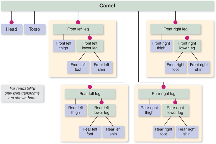
Figure 6.49: Scene graph of a camel constructed without reusable components, allowing individual control of each joint.
Is any “reuse” going on in this model? Well, you could say that we are reusing the design of the leg, since the model has four copies of the leg component hierarchy we designed above. But there is no reuse of the actual components in the constructed model. The front-left leg is a tree of components dedicated to representing only the front-left leg; there is a completely independent tree of components for each of the four legs. The advantage of this approach is that each leg is independent of the others, and the effect of manipulating one leg’s joints is limited in scope to just that leg.
It is useful to search a model for rigid subcomponents that do not have any internal joints; they are candidates for being extracted and turned into reusable components. In the model discussed above, the lower-leg component is indeed rigid, because our design does not include an ankle joint that would allow the foot to rotate relative to the shin. Thus, we can reuse the lower-leg component hierarchy without any loss of animation flexibility, by constructing the camel using the structure shown in Figure 6.50. Here, our model is no longer a tree—it is a directed acyclic graph (DAG) now that component reuse is in effect; this topology is the reason this kind of structure is known as a “scene graph.”
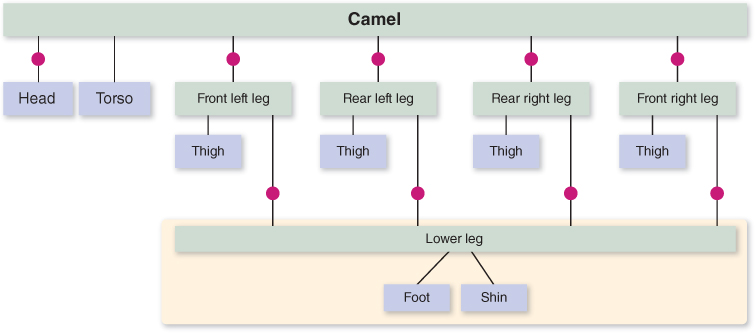
Figure 6.50: Reducing the storage cost by reusing a lower-leg submodel, with no loss of flexibility in joint control.
As the figure makes clear, each instantiation of the reusable LowerLeg has its own knee joint transform, so there is no loss in flexibility—each knee joint is still individually controllable. This DAG-based design is identical in functionality to the tree-based design above.
Thus far, we have been focused on supporting a high-fidelity animation of the camel’s movement, but there other scenarios of interest. Consider a desert scene in which hundreds of camels, seen from afar, are crossing dunes in a caravan. The amount of processing needed to animate each hip and knee joint individually might be considered not worth the cost, especially if the caravan is so far from the viewpoint that such details would not be apparent to the viewer. In such a case, we might choose a lower-fidelity motion in which the camels move in unison, with all left legs, both front and back, in the scene sharing a particular knee-bend animation, and all right legs sharing a different knee-bend animation.
A model using this approach is depicted in Figure 6.51. Here we have our first reusable components that include internal joint transforms: The reusable left leg has a left-knee joint, and the reusable right leg has its own right-knee joint. If we were to do a test instantiation of just one camel designed in this way, we would be able to control both left knees by manipulating just the one left-knee joint transform, and both right knees via the one right-knee joint transform.
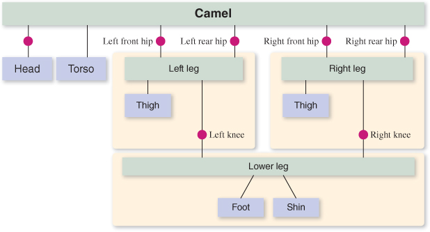
Figure 6.51: Reducing the storage cost by reusing a model for the left-side legs and a separate model for the right-side legs, with great loss of flexibility in joint control.
But the processing advantage gained by reuse becomes much more apparent if you increase the number of camels to simulate the entire caravan. Consider Figure 6.52, which depicts a model of a caravan featuring reuse of the entire camel model.
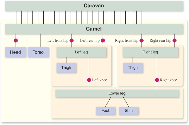
Figure 6.52: Modeling a caravan by reusing a single camel model, a highly scalable approach at the cost of excessive synchronized leg movement.
With this new scene graph, we have a caravan that is extremely scalable. No matter how many camels we place in this caravan, the number of joint transforms requiring manipulation for the animation of the legs is constant. By manipulating just four hip joints and two knee joints, the entire caravan’s leg motion will be affected. Of course, this scalability comes at a cost: the uncanny and unnatural perfect synchronization of the entire caravan. At a distance, this type of low-fidelity caravan might be perfectly adequate, but if a bit more variety is desired, we could choose to have a handful of different limb animation sequences, create a distinct reusable camel “stencil” for each such sequence, and have each camel in the caravan be an instance of one of the stencils, chosen at random. Without much loss in scalability, we could thus achieve animation that is not quite so unnatural.
Of course, our caravan needs to be moving across the desert too; otherwise, the leg motions will look awfully silly. Thus, our animation logic must perform time-based manipulation of instance transforms on the camel objects simultaneously with the manipulation of the joint transforms.
How can we make the caravan’s movement across the desert scalable? Is there a scene graph that would allow a single instance transform to move the entire caravan, without the loss of the scalable knee/hip control we just designed? What loss in realism would occur with such a plan?
If you are interested in knowing more about how to implement reusable components in XAML and WPF, consult the online materials for this chapter.
WPF is, of course, just one of many scene-graph platforms, and all implement reusability as part of their support for controlling scene complexity. For more information on scene-graph platforms, see Chapter 16.
6.7. Discussion
We have demonstrated the techniques common to most real-time fixed-function 3D platforms that are useful for displaying simple scenes composed of triangle-mesh objects, covered with solid or texture-mapped materials, and rendered using the classic Phong reflectance model with interpolated or flat shading.
Our focus on WPF as the example platform is designed to allow you to experiment and build prototype scenes using XAML, so you can exercise these techniques without the need to work with a procedural language and compile/build cycles.
It is important to note that a platform-resident scene graph is only applicable to projects for which “the picture is the thing.” For most nontrivial applications, where the image is meant to be a visualization of some application data, there is an application model (database) storing both geometric and nongeometric information, acting as the source from which a scene graph is derived for display purposes. This topic is discussed more extensively in Chapter 16.