
Chapter 10. Transformations in Two Dimensions
10.1. Introduction
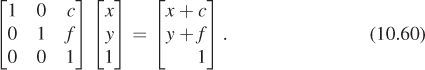
As you saw in Chapters 2 and 6, when we think about taking an object for which we have a geometric model and putting it in a scene, we typically need to do three things: Move the object to some location, scale it up or down so that it fits well with the other objects in the scene, and rotate it until it has the right orientation. These operations—translation, scaling, and rotation—are part of every graphics system. Both scaling and rotation are linear transformations on the coordinates of the object’s points. Recall that a linear transformation,
is one for which T(v + αw) = T(v) + αT(w) for any two vectors v and w in R2, and any real number α. Intuitively, it’s a transformation that preserves lines and leaves the origin unmoved.
Suppose T is linear. Insert α = 1 in the definition of linearity. What does it say? Insert v = 0 in the definition. What does it say?
When we say that a linear transformation “preserves lines,” we mean that if ![]() is a line, then the set of points T(
is a line, then the set of points T(![]() ) must also lie in some line. You might expect that we’d require that T(
) must also lie in some line. You might expect that we’d require that T(![]() ) actually be a line, but that would mean that transformations like “project everything perpendicularly onto the x-axis” would not be counted as “linear.” For this particular projection transformation, describe a line
) actually be a line, but that would mean that transformations like “project everything perpendicularly onto the x-axis” would not be counted as “linear.” For this particular projection transformation, describe a line ![]() such that T(
such that T(![]() ) is contained in a line, but is not itself a line.
) is contained in a line, but is not itself a line.
The definition of linearity guarantees that for any linear transformation T, we have T(0) = 0: If we choose v = w = 0 and α = 1, the definition tells us that
Subtracting T(0) from the first and last parts of this chain gives us 0 = T(0). This means that translation—moving every point of the plane by the same amount—is, in general, not a linear transformation except in the special case of translation by zero, in which all points are left where they are. Shortly we’ll describe a trick for putting the Euclidean plane into R3 (but not as the z = 0 plane as is usually done); once we do this, we’ll see that certain linear transformations on R3 end up performing translations on this embedded plane.
For now, let’s look at only the plane. We assume that you have some familiarity with linear transformations already; indeed, the serious student of computer graphics should, at some point, study linear algebra carefully. But one can learn a great deal about graphics with only a modest amount of knowledge of the subject, which we summarize here briefly.
In the first few sections, we use the convention of most linear-algebra texts:
The vectors are arrows at the origin, and we think of the vector ![]() as being identified with the point (u, v). Later we’ll return to the point-vector distinction.
as being identified with the point (u, v). Later we’ll return to the point-vector distinction.
For any 2 × 2 matrix M, the function v ![]() Mv is a linear transformation from R2 to R2. We refer to this as a matrix transformation. In this chapter, we look at five such transformations in detail, study matrix transformations in general, and introduce a method for incorporating translation into the matrix-transformation formulation. We then apply these ideas to transforming objects and changing coordinate systems, returning to the clock example of Chapter 2 to see the ideas in practice.
Mv is a linear transformation from R2 to R2. We refer to this as a matrix transformation. In this chapter, we look at five such transformations in detail, study matrix transformations in general, and introduce a method for incorporating translation into the matrix-transformation formulation. We then apply these ideas to transforming objects and changing coordinate systems, returning to the clock example of Chapter 2 to see the ideas in practice.
10.2. Five Examples
We begin with five examples of linear transformations in the plane; we’ll refer to these by the names T1, ..., T5 throughout the chapter.
Example 1: Rotation. Let ![]()
and
Recall that e1 denotes the vector ![]() and
and ![]() ; this transformation sends e1 to the vector
; this transformation sends e1 to the vector ![]() and e2 to
and e2 to ![]() , which are vectors that are 30° counterclockwise from the x- and y-axes, respectively (see Figure 10.1).
, which are vectors that are 30° counterclockwise from the x- and y-axes, respectively (see Figure 10.1).
There’s nothing special about the number 30 in this example; by replacing 30° with any angle, you can build a transformation that rotates things counterclockwise by that angle.
Write down the matrix transformation that rotates everything in the plane by 180° counterclockwise. Actually compute the sines and cosines so that you end up with a matrix filled with numbers in your answer. Apply this transformation to the corners of the unit square, (0, 0), (1, 0), (0, 1), and (1, 1).
Example 2: Nonuniform scaling. Let ![]() and
and
This transformation stretches everything by a factor of three in the x-direction and a factor of two in the y-direction, as shown in Figure 10.2. If both stretch factors were three, we’d say that the transformation “scaled things up by three” and is a uniform scaling transformation. T2 represents a generalization of this idea: Rather than scaling uniformly in each direction, it’s called a nonuniform scaling transformation or, less formally, a nonuniform scale.
Once again the example generalizes: By placing numbers other than 2 and 3 along the diagonal of the matrix, we can scale each axis by any amount we please. These scaling amounts can include zero and negative numbers.
Write down the matrix for a uniform scale by –1. How does your answer relate to your answer to inline Exercise 10.3? Can you explain?
Write down a transformation matrix that scales in x by zero and in y by 1. Informally describe what the associated transformation does to the house.
Example 3: Shearing. Let ![]() and
and
As Figure 10.3 shows, T3 preserves height along the y-axis but moves points parallel to the x-axis, with the amount of movement determined by the y-value. The x-axis itself remains fixed. Such a transformation is called a shearing transformation.
Generalize to build a transformation that keeps the y-axis fixed but shears vertically instead of horizontally.
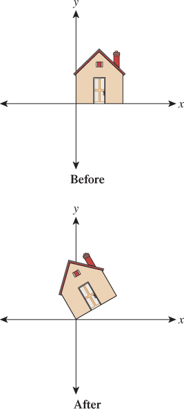
Example 4: A general transformation. Let ![]() and
and
Figure 10.4 shows the effects of T4. It distorts the house figure, but not by just a rotation or scaling or shearing along the coordinate axes.
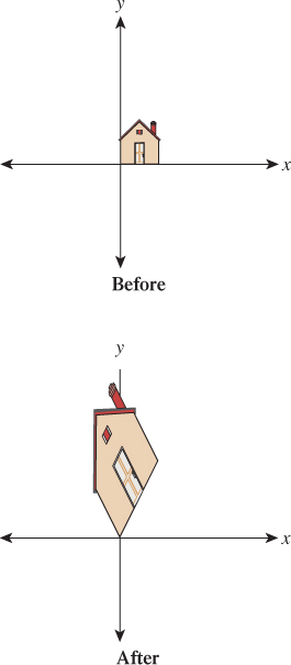
Figure 10.4: A general transformation. The house has been quite distorted, in a way that’s hard to describe simply, as we’ve done for the earlier examples.
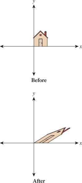
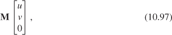
Example 5: A degenerate (or singular) transformation Let
Figure 10.5 shows why we call this transformation degenerate: Unlike the others, it collapses the whole two-dimensional plane down to a one-dimensional subspace, a line. There’s no longer a nice correspondence between points in the domain and points in the codomain: Certain points in the codomain no longer correspond to any point in the domain; others correspond to many points in the domain. Such a transformation is also called singular, as is the matrix defining it. Those familiar with linear algebra will note that this is equivalent to saying that the determinant of ![]() is zero, or saying that its columns are linearly dependent.
is zero, or saying that its columns are linearly dependent.
10.3. Important Facts about Transformations
Here we’ll describe several properties of linear transformations from R2 to R2. These properties are important in part because they all generalize: They apply (in some form) to transformations from Rn to Rk for any n and k. We’ll mostly be concerned with values of n and k between 1 and 4; in this section, we’ll concentrate on n = k = 2.
10.3.1. Multiplication by a Matrix Is a Linear Transformation
If M is a 2 × 2 matrix, then the function TM defined by
is linear. All five examples above demonstrate this.
For nondegenerate transformations, lines are sent to lines, as T1 through T4 show. For degenerate ones, a line may be sent to a single point. For instance, T5 sends the line consisting of all vectors of the form ![]() to the zero vector.
to the zero vector.
Because multiplication by a matrix M is always a linear transformation, we’ll call TM the transformation associated to the matrix M.
10.3.2. Multiplication by a Matrix Is the Only Linear Transformation
In Rn, it turns out that for every linear transform T, there’s a matrix M with T(x) = Mx, which means that every linear transformation is a matrix transformation. We’ll see in Section 10.3.5 how to find M, given T, even if T is expressed in some other way. This will show that the matrix M is completely determined by the transformation T, and we can thus call it the matrix associated to the transformation.
As a special example, the matrix I, with ones on the diagonal and zeroes off the diagonal, is called the identity matrix; the associated transformation
is special: It’s the identity transformation that leaves every vector x unchanged.
There is an identity matrix of every size: a 1 × 1 identity, a 2 × 2 identity, etc. Write out the first three.
10.3.3. Function Composition and Matrix Multiplication Are Related
If M and K are 2 × 2 matrices, then they define transformations TM and TK. When we compose these, we get the transformation
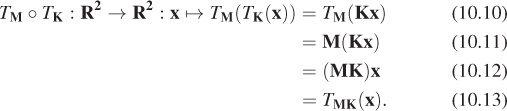
In other words, the composed transformation is also a matrix transformation, with matrix MK. Note that when we write TM(TK(x)), the transformation TK is applied first. So, for example, if we look at the transformation T2 ο T3, it first shears the house and then scales the result nonuniformly.
Describe the appearance of the house after transforming it by T1 ο T2 and after transforming it by T2 ο T1.
10.3.4. Matrix Inverse and Inverse Functions Are Related
A matrix M is invertible if there’s a matrix B with the property that BM = MB = I. If such a matrix exists, it’s denoted M–1.
If M is invertible and S(x) = M– 1x, then S is the inverse function of TM, that is,
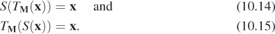
If M is not invertible, then TM has no inverse.
Let’s look at our examples. The matrix for T1 has an inverse: Simply replace 30 by −30 in all the entries. The resultant transformation rotates clockwise by 30°; performing one rotation and then the other effectively does nothing (i.e., it is the identity transformation). The inverse for the matrix for T2 is diagonal, with entries ![]() and
and ![]() . The inverse of the matrix for T3 is
. The inverse of the matrix for T3 is ![]() (note the negative sign). The associated transformation also shears parallel to the x-axis, but vectors in the upper half-plane are moved to the left, which undoes the moving to the right done by T3.
(note the negative sign). The associated transformation also shears parallel to the x-axis, but vectors in the upper half-plane are moved to the left, which undoes the moving to the right done by T3.
For these first three it was fairly easy to guess the inverse matrices, because we could understand how to invert the transformation. The inverse of the matrix for T4 is
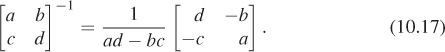
which we computed using a general rule for inverses of 2 × 2 matrices (the only such rule worth memorizing):
Finally, for T5, the matrix has no inverse; if it did, the function T5 would be invertible: It would be possible to identify, for each point in the codomain, a single point in the domain that’s sent there. But we’ve already seen this isn’t possible.
Apply the formula from Equation 10.17 to the matrix for T5 to attempt to compute its inverse. What goes wrong?
10.3.5. Finding the Matrix for a Transformation
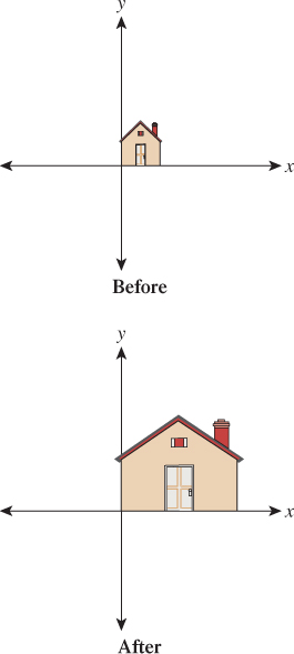
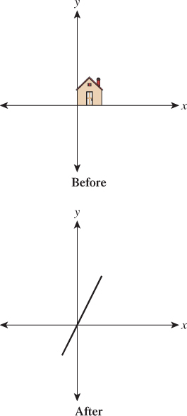
We’ve said that every linear transformation really is just multiplication by some matrix, but how do we find that matrix? Suppose, for instance, that we’d like to find a linear transformation to flip our house across the y-axis so that the house ends up on the left side of the y-axis. (Perhaps you can guess the transformation that does this, and the associated matrix, but we’ll work through the problem directly.)
The key idea is this: If we know where the transformation sends e1 and e2, we know the matrix. Why? We know that the transformation must have the form
we just don’t know the values of a, b, c, and d. Well, T(e1) is then
Similarly, T(e2) is the vector ![]() . So knowing T(e1) and T(e2) tells us all the matrix entries. Applying this to the problem of flipping the house, we know that T(e1) = – e1, because we want a point on the positive x-axis to be sent to the corresponding point on the negative x-axis, so a = –1 and c = 0. On the other hand, T(e2) = e2, because every vector on the y-axis should be left untouched, so b = 0 and d = 1. Thus, the matrix for the house-flip transformation is just
. So knowing T(e1) and T(e2) tells us all the matrix entries. Applying this to the problem of flipping the house, we know that T(e1) = – e1, because we want a point on the positive x-axis to be sent to the corresponding point on the negative x-axis, so a = –1 and c = 0. On the other hand, T(e2) = e2, because every vector on the y-axis should be left untouched, so b = 0 and d = 1. Thus, the matrix for the house-flip transformation is just
(a) Find a matrix transformation sending e1 to ![]() and e2 to
and e2 to ![]() .
.
(b) Use the relationship of matrix inverse to the inverse of a transform, and the formula for the inverse of a 2 × 2 matrix, to find a transformation sending ![]() to e1 and
to e1 and ![]() to e2 as well.
to e2 as well.
As Inline Exercise 10.11 shows, we now have the tools to send the standard basis vectors e1 and e2 to any two vectors v1 and v2, and vice versa (provided that v1 and v2 are independent, that is, neither is a multiple of the other). We can combine this with the idea that composition of linear transformations (performing one after the other) corresponds to multiplication of matrices and thus create a solution to a rather general problem.
Problem: Given independent vectors u1 and u2 and any two vectors v1 and v2, find a linear transformation, in matrix form, that sends u1 to v1 and u2 to v2.
Solution: Let M be the matrix whose columns are u1 and u2. Then
sends e1 to u1 and e2 to u2 (see Figure 10.6). Therefore,
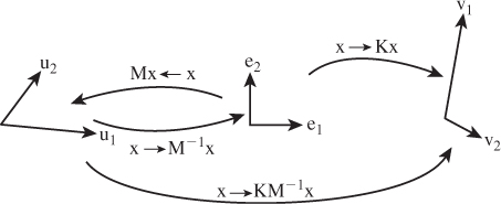
Figure 10.6: Multiplication by the matrix M takes e1 and e2 to u1 and u2, respectively, so multiplying M–1 does the opposite. Multiplying by K takes e1 and e2 to v1 and v2, so multiplying first by M– 1and then by K, that is, multiplying by KM–1, takes u1 to e1 to v1, and similarly for u2.
sends u1 to e1 and u2 to e2.
Now let K be the matrix with columns v1 and v2. The transformation
sends e1 to v1 and e2 to v2.
If we apply first S and then R to u1, it will be sent to e1 (by S), and thence to v1 by R; a similar argument applies to u2. Writing this in equations,
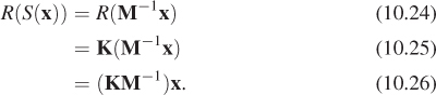
Thus, the matrix for the transformation sending the u’s to the v’s is just KM–1.
Let’s make this concrete with an example. We’ll find a matrix sending
to
respectively. Following the pattern above, the matrices M and K are
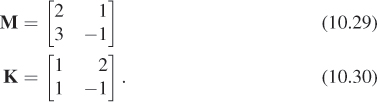
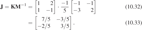
Using the matrix inversion formula (Equation 10.17), we find
so that the matrix for the overall transformation is
As you may have guessed, the kinds of transformations we used in WPF in Chapter 2 are internally represented as matrix transformations, and transformation groups are represented by sets of matrices that are multiplied together to generate the effect of the group.
Verify that the transformation associated to the matrix J in Equation 10.32 really does send u1 to v1 and u2 to v2.
Let ![]() and
and ![]() ; pick any two nonzero vectors you like as v1 and v2, and find the matrix transformation that sends each ui to the corresponding vi.
; pick any two nonzero vectors you like as v1 and v2, and find the matrix transformation that sends each ui to the corresponding vi.
The recipe above for building matrix transformations shows the following: Every linear transformation from R2 to R2 is determined by its values on two independent vectors. In fact, this is a far more general property: Any linear transformation from R2 to Rk is determined by its values on two independent vectors, and indeed, any linear transformation from Rn to Rk is determined by its values on n independent vectors (where to make sense of these, we need to extend our definition of “independence” to more than two vectors, which we’ll do presently).
10.3.6. Transformations and Coordinate Systems
We tend to think about linear transformations as moving points around, but leaving the origin fixed; we’ll often use them that way. Equally important, however, is their use in changing coordinate systems. If we have two coordinate systems on R2 with the same origin, as in Figure 10.7, then every arrow has coordinates in both the red and the blue systems. The two red coordinates can be written as a vector, as can the two blue coordinates. The vector u, for instance, has coordinates ![]() in the red system and approximately
in the red system and approximately ![]() in the blue system.
in the blue system.

Figure 10.7: Two different coordinate systems for R2; the vector u, expressed in the red coordinate system, has coordinates 3 and 2, indicated by the dotted lines, while the coordinates in the blue coordinate system are approximately −0.2 and 3.6, where we’ve drawn, in each case, the positive side of the first coordinate axis in bold.
Use a ruler to find the coordinates of r and s in each of the two coordinate systems.
We could tabulate every imaginable arrow’s coordinates in the red and blue systems to convert from red to blue coordinates. But there is a far simpler way to achieve the same result. The conversion from red coordinates to blue coordinates is linear and can be expressed by a matrix transformation. In this example, the matrix is
Multiplying M by the coordinates of u in the red system gets us
which is the coordinate vector for u in the blue system.
Confirm, for each of the other arrows in Figure 10.7, that the same transformation converts red to blue coordinates.
By the way, when creating this example we computed M just as we did at the start of the preceding section: We found the blue coordinates of each of the two basis vectors for the red coordinate system, and used these as the columns of M.
In the special case where we want to go from the usual coordinates on a vector to its coordinates in some coordinate system with basis vectors u1, u2, which are unit vectors and mutually perpendicular, the transformation matrix is one whose rows are the transposes of u1 and u2.
For example, if ![]() and
and ![]() (check for yourself that these are unit length and perpendicular), then the vector
(check for yourself that these are unit length and perpendicular), then the vector ![]() , expressed in u-coordinates, is
, expressed in u-coordinates, is
Verify for yourself that these really are the u-coordinates of v, that is, that the vector v really is the same as 4u1 + (–2) u2.
10.3.7. Matrix Properties and the Singular Value Decomposition
Because matrices are so closely tied to linear transformations, and because linear transformations are so important in graphics, we’ll now briefly discuss some important properties of matrices.
First, diagonal matrices—ones with zeroes everywhere except on the diagonal, like the matrix M2 for the transformation T2—correspond to remarkably simple transformations: They just scale up or down each axis by some amount (although if the amount is a negative number, the corresponding axis is also flipped). Because of this simplicity, we’ll try to understand other transformations in terms of these diagonal matrices.
Second, if the columns of the matrix M are v1, v2, ..., vk ![]() Rn, and they are pairwise orthogonal unit vectors, then MTM = Ik, the k × k identity matrix.
Rn, and they are pairwise orthogonal unit vectors, then MTM = Ik, the k × k identity matrix.
In the special case where k = n, such a matrix is called orthogonal. If the determinant of the matrix is 1, then the matrix is said to be a special orthogonal matrix. In R2, such a matrix must be a rotation matrix like the one in T1; in R3, the transformation associated to such a matrix corresponds to rotation around some vector by some amount.1
1. As we mentioned in Chapter 3, rotation about a vector in R3 is better expressed as rotation in a plane, so instead of speaking about rotation about z, we speak of rotation in the xy-plane. We can then say that any special orthogonal matrix in R4 corresponds to a sequence of two rotations in two planes in 4-space.
Less familiar to most students, but of enormous importance in much graphics research, is the singular value decomposition (SVD) of a matrix. Its existence says, informally, that if we have a transformation T represented by a matrix M, and if we’re willing to use new coordinate systems on both the domain and codomain, then the transformation simply looks like a nonuniform (or possibly uniform) scaling transformation. We’ll briefly discuss this idea here, along with the application of the SVD to solving equations; the web materials for this chapter show the SVD for our example transformations and some further applications of the SVD.
The singular value decomposition theorem says this:
Every n × k matrix M can be factored in the form
where U is n × r (where r = min(n, k)) with orthonormal columns, D is r × r diagonal (i.e., only entries of the form dii can be nonzero), and V is r × k with orthonormal columns (see Figure 10.8).
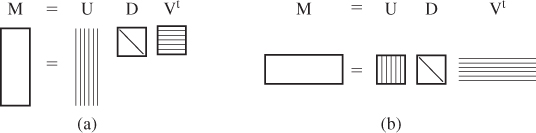
Figure 10.8: (a) An n × k matrix, with n > k, factors as a product of an n × n matrix with orthonormal columns (indicated by the vertical stripes on the first rectangle), a diagonal k×k matrix, and a k×k matrix with orthonormal rows (indicated by the horizontal stripes), which we write as UDVT, where U and V have orthonormal columns. (b) An n × k matrix with n < k is written as a similar product; note that the diagonal matrix in both cases is square, and its size is the smaller of n and k.
By convention, the entries of D are required to be in nonincreasing order (i.e., |d1,1| ≥ |d2,2| ≥ |d3,3| ...) and are indicated by single subscripts (i.e., we write d1 instead of d1,1). They are called the singular values of M. It turns out that M is degenerate (i.e., singular) exactly if any singular value is 0. As a general guideline, if the ratio of the largest to the smallest singular values is very large (say, 106), then numerical computations with the matrix are likely to be unstable.
The singular value decomposition is not unique. If we negate the first row of VT and the first column of U in the SVD of a matrix M, show that the result is still an SVD for M.
In the special case where n = k (the one we most often encounter), the matrices U and V are both square and represent change-of-coordinate transformations in the domain and codomain. Thus, we can see the transformation
as a sequence of three steps: (1) Multiplication by VT converts x to v-coordinates; (2) multiplication by D amounts to a possibly nonuniform scaling along each axis; and (3) multiplication by U treats the resultant entries as coordinates in the u-coordinate system, which then are transformed back to standard coordinates.
10.3.8. Computing the SVD
How do we find U, D, and V? In general it’s relatively difficult, and we rely on numerical linear algebra packages to do it for us. Furthermore, the results are by no means unique: A single matrix may have multiple singular value decompositions. For instance, if S is any n × n matrix with orthonormal columns, then
is one possible singular value decomposition of the identity matrix. Even though there are many possible SVDs, the singular values are the same for all decompositions.
The rank of the matrix M, which is defined as the number of linearly independent columns, turns out to be exactly the number of nonzero singular values.
10.3.9. The SVD and Pseudoinverses
Again, in the special case where n = k so that U and V are square, it’s easy to compute M–1 if you know the SVD:
where D−1 is easy to compute—you simply invert all the elements of the diagonal. If one of these elements is zero, the matrix is singular and no such inverse exists; in this case, the pseudoinverse is also often useful. It’s defined as
where D† is just D with every nonzero entry inverted (i.e., you try to invert the diagonal matrix D by inverting diagonal elements, and every time you encounter a zero on the diagonal, you ignore it and simply write down 0 in the answer). The definition of the pseudoinverse makes sense even when n ≠ k; the pseudoinverse can be used to solve “least squares” problems, which frequently arise in graphics.
The Pseudoinverse Theorem:
(a) If M is an n × k matrix with n >k, the equation Mx = b generally represents an overdetermined system of equations2 which may have no solution. The vector
2. In other words, a situation like “five equations in three unknowns.”
represents an optimal “solution” to this system, in the sense that Mx0 is as close to b as possible.
(b) If M is an n × k matrix with n < k, and rank n, the equation Mx = b represents an underdetermined system of equations.3 The vector
3. That is, a situation like “three equations in five unknowns.”
represents an optimal solution to this system, in the sense that x0 is the shortest vector satisfying Mx = b.
Here are examples of each of these cases.
Example 1: An overdetermined system
The system
has no solution: There’s simply no number t with 2t = 4 and 1t = 3 (see Figure 10.9). But among all the multiples of ![]() , there is one that’s closest to the vector
, there is one that’s closest to the vector ![]() , namely
, namely ![]() , as you can discover with elementary geometry. The theorem tells us we can compute this directly, however, using the pseudoinverse. The SVD and pseudoinverse of M are
, as you can discover with elementary geometry. The theorem tells us we can compute this directly, however, using the pseudoinverse. The SVD and pseudoinverse of M are
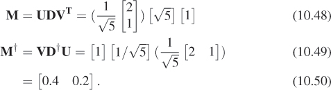
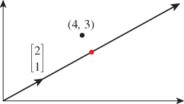
Figure 10.9: The equations ![]() have no common solution. But the multiples of the vector [2 1]T form a line in the plane that passes by the point (4, 3), and there’s a point of this line (shown in a red circle on the topmost arrow) that’s as close to (4, 3) as possible.
have no common solution. But the multiples of the vector [2 1]T form a line in the plane that passes by the point (4, 3), and there’s a point of this line (shown in a red circle on the topmost arrow) that’s as close to (4, 3) as possible.
And the solution guaranteed by the theorem is
Example 2: An underdetermined system
The system
has a great many solutions; any point (x, y) on the line x + 3y = 4 is a solution (see Figure 10.10). The solution that’s closest to the origin is the point on the line x + 3y = 4 that’s as near to (0, 0) as possible, which turns out to be x = 0.4; y = 1.2. In this case, the matrix M is [1 3]; its SVD and pseudoinverse are simply
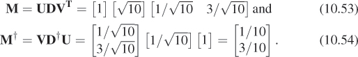
And the solution guaranteed by the theorem is
Of course, this kind of computation is much more interesting in the case where the matrices are much larger, but all the essential characteristics are present even in these simple examples.
A particularly interesting example arises when we have, for instance, two polyhedral models (consisting of perhaps hundreds of vertices joined by triangular faces) that might be “essentially identical”: One might be just a translated, rotated, and scaled version of the other. In Section 10.4, we’ll see how to represent translation along with rotation and scaling in terms of matrix multiplication. We can determine whether the two models are in fact essentially identical by listing the coordinates of the first in the columns of a matrix V and the coordinates of the second in a matrix W, and then seeking a matrix A with
This amounts to solving the “overconstrained system” problem; we find that A = V†W is the best possible solution. If, having computed A, we find that
then the models are essentially identical; if the left and right sides differ, then the models are not essentially identical. (This entire approach depends, of course, on corresponding vertices of the two models being listed in the corresponding order; the more general problem is a lot more difficult.)
10.4. Translation
We now describe a way to apply linear transformations to generate translations, and at the same time give a nice model for the points-versus-vectors ideas we’ve espoused so far.
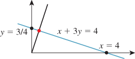
The idea is this: As our Euclidean plane (our set of points), we’ll take the plane w = 1 in xyw-space (see Figure 10.11). The use of w here is in preparation for what we’ll do in 3-space, which is to consider the three-dimensional set defined by w = 1 in xyzw-space.
Having done this, we can consider transformations that multiply such vectors by a 3 × 3 matrix M. The only problem is that the result of such a multiplication may not have a 1 as its last entry. We can restrict our attention to those that do:
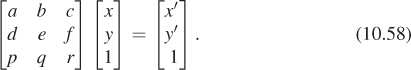
For this equation to hold for every x and y, we must have px + qy + r = 1 for all x, y. This forces p = q = 0 and r = 1.
Thus, we’ll consider transformations of the form
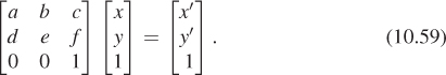
If we examine the special case where the upper-left corner is a 2 × 2 identity matrix, we get
As long as we pay attention only to the x- and y-coordinates, this looks like a translation! We’ve added c to each x-coordinate and f to each y-coordinate (see Figure 10.12). Transformations like this, restricted to the plane w = 1, are called affine transformations of the plane. Affine transformations are the ones most often used in graphics.
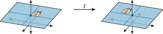
Figure 10.12: The house figure, before and after a translation generated by shearing parallel to the w = 1 plane.
On the other hand, if we make c = f = 0, then the third coordinate becomes irrelevant, and the upper-left 2 × 2 matrix can perform any of the operations we’ve seen up until now. Thus, with the simple trick of adding a third coordinate and requiring that it always be 1, we’ve managed to unify rotation, scaling, and all the other linear transformations with the new class of transformations, translations, to get the class of affine transformations.
10.5. Points and Vectors Again
Back in Chapter 7, we said that points and vectors could be combined in certain ways: The difference of points is a vector, a vector could be added to a point to get a new point, and more generally, affine combinations of points, that is, combinations of the form
were allowed if and only if α1 + α2 + ... + αk = 1.
We now have a situation in which these distinctions make sense in terms of familiar mathematics: We can regard points of the plane as being elements of R3 whose third coordinate is 1, and vectors as being elements of R3 whose third coordinate is 0.
With this convention, it’s clear that the difference of points is a vector, the sum of a vector and a point is a point, and combinations like the one in Equation 10.61 yield a point if and only if the sum of the coefficients is 1 (because the third coordinate of the result will be exactly the sum of the coefficients; for the sum to be a point, this third coordinate is required to be 1).
You may ask, “Why, when we’re already familiar with vectors in 3-space, should we bother calling some of them ‘points in the Euclidean plane’ and others ‘two-dimensional vectors’?” The answer is that the distinctions have geometric significance when we’re using this subset of 3-space as a model for 2D transformations. Adding vectors in 3-space is defined in linear algebra, but adding together two of our “points” gives a location in 3-space that’s not on the w = 1 plane or the w = 0 plane, so we don’t have a name for it at all.
Henceforth we’ll use E2 (for “Euclidean two-dimensional space”) to denote this w = 1 plane in xyw-space, and we’ll write (x, y) to mean the point of E2 corresponding to the 3-space vector ![]() . It’s conventional to speak of an affine transformation as acting on E2, even though it’s defined by a 3 × 3 matrix.
. It’s conventional to speak of an affine transformation as acting on E2, even though it’s defined by a 3 × 3 matrix.
10.6. Why Use 3 × 3 Matrices Instead of a Matrix and a Vector?
Students sometimes wonder why they can’t just represent a linear transformation plus translation in the form
where the matrix M represents the linear part (rotating, scaling, and shearing) and b represents the translation.
First, you can do that, and it works just fine. You might save a tiny bit of storage (four numbers for the matrix and two for the vector, so six numbers instead of nine), but since our matrices always have two 0s and a 1 in the third row, we don’t really need to store that column anyhow, so it’s the same. Otherwise, there’s no important difference.
Second, the reason to unify the transformations into a single matrix is that it’s then very easy to take multiple transformations (each represented by a matrix) and compose them (perform one after another): We just multiply their matrices together in the right order to get the matrix for the composed transformation. You can do this in the matrix-and-vector formulation as well, but the programming is slightly messier and more error-prone.
There’s a third reason, however: It’ll soon become apparent that we can also work with triples whose third entry is neither 1 nor 0, and use the operation of homogenization (dividing by w) to convert these to points (i.e., triples with w = 1), except when w = 0. This allows us to study even more transformations, one of which is central to the study of perspective, as we’ll see later.
The singular value decomposition provides the tool necessary to decompose not just linear transformations, but affine ones as well (i.e., combinations of linear transformations and translations).
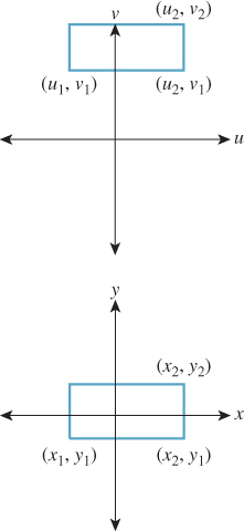
10.7. Windowing Transformations
As an application of our new, richer set of transformations, let’s examine windowing transformations, which send one axis-aligned rectangle to another, as shown in Figure 10.13. (We already discussed this briefly in Chapter 3.)
We’ll first take a direct approach involving a little algebra. We’ll then examine a more automated approach.
We’ll need to do essentially the same thing to the first and second coordinates, so let’s look at how to transform the first coordinate only. We need to send u1 to x1 and u2 to x2. That means we need to scale up any coordinate difference by the factor ![]() . So our transformation for the first coordinate has the form
. So our transformation for the first coordinate has the form
If we apply this to t = u1, we know that we want to get x1; this leads to the equation
Solving for the missing offset gives
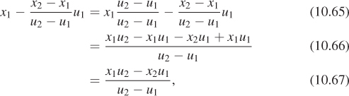
so that the transformation is
Doing essentially the same thing for the v and y terms (i.e., the second coordinate) we get the transformation, which we can write in matrix form:
where
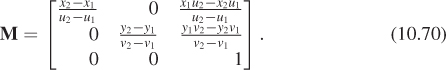
Multiply the matrix M of Equation 10.70 by the vector [u1 v1 1]T to confirm that you do get [x1 y1 1]T. Do the same for the opposite corner of the rectangle.
We’ll now show you a second way to build this transformation (and many others as well).
10.8. Building 3D Transformations
Recall that in 2D we could send the vectors e1 and e2 to the vectors v1 and v2 by building a matrix M whose columns were v1 and v2, and then use two such matrices (inverting one along the way) to send any two independent vectors v1 and v2 to any two vectors w1 and w2. We can do the same thing in 3-space: We can send the standard basis vectors e1, e2, and e3 to any three other vectors, just by using those vectors as the columns of a matrix. Let’s start by sending e1, e2, and e3 to three corners of our first rectangle—the two we’ve already specified and the lower-right one, at location (u2, v1). The three vectors corresponding to these points are
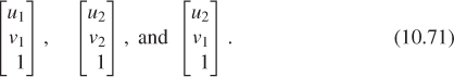
Because the three corners of the rectangle are not collinear, the three vectors are independent. Indeed, this is our definition of independence for vectors in n-space: Vectors v1, ..., vk are independent if there’s no (k–1)-dimensional subspace containing them. In 3-space, for instance, three vectors are independent if there’s no plane through the origin containing all of them.
So the matrix
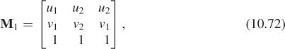
which performs the desired transformation, will be invertible.
We can similarly build the matrix M2, with the corresponding xs and ys in it. Finally, we can compute
which will perform the desired transformation. For instance, the lower-left corner of the starting rectangle will be sent, by ![]() , to e1 (because M1 sent e1 to the lower-left corner); multiplying e1 by M2 will send it to the lower-left corner of the target rectangle. A similar argument applies to all three corners. Indeed, if we compute the inverse algebraically and multiply out everything, we’ll once again arrive at the matrix given in Equation 10.7. But we don’t need to do so: We know that this must be the right matrix. Assuming we’re willing to use a matrix-inversion routine, there’s no need to think through anything more than “I want these three points to be sent to these three other points.”
, to e1 (because M1 sent e1 to the lower-left corner); multiplying e1 by M2 will send it to the lower-left corner of the target rectangle. A similar argument applies to all three corners. Indeed, if we compute the inverse algebraically and multiply out everything, we’ll once again arrive at the matrix given in Equation 10.7. But we don’t need to do so: We know that this must be the right matrix. Assuming we’re willing to use a matrix-inversion routine, there’s no need to think through anything more than “I want these three points to be sent to these three other points.”
Summary: Given any three noncollinear points P1, P2, P3 in E2, we can find a matrix transformation and send them to any three points Q1, Q2, Q3 with the procedure above.
10.9. Another Example of Building a 2D Transformation
Suppose we want to find a 3 × 3 matrix transformation that rotates the entire plane 30° counterclockwise around the point P = (2, 4), as shown in Figure 10.14. As you’ll recall, WPF expresses this transformation via code like this:
<RotateTransform Angle="-30" CenterX="2" CenterY="4"/>
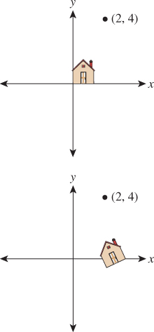
Figure 10.14: We’d like to rotate the entire plane by 30° counterclockwise about the point P = (2, 4).
An implementer of WPF then must create a matrix like the one we’re about to build.
Here are two approaches.
First, we know how to rotate about the origin by 30°; we can use the transformation T1 from the start of the chapter. So we can do our desired transformation in three steps (see Figure 10.15).
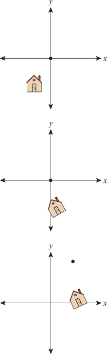
Figure 10.15: The house after translating (2, 4) to the origin, after rotating by 30°, and after translating the origin back to (2, 4).
1. Move the point (2, 4) to the origin.
2. Rotate by 30°.
3. Move the origin back to (2, 4).
The matrix that moves the point (2, 4) to the origin is
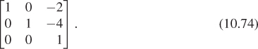
The one that moves it back is similar, except that the 2 and 4 are not negated. And the rotation matrix (expressed in our new 3 × 3 format) is
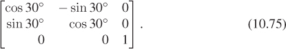
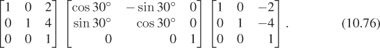
The matrix representing the entire sequence of transformations is therefore
(a) Explain why this is the correct order in which to multiply the transformations to get the desired result.
(b) Verify that the point (2, 4) is indeed left unmoved by multiplying [2 4 1]T by the sequence of matrices above.
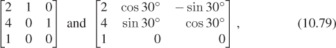
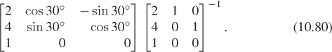
The second approach is again more automatic: We find three points whose target locations we know, just as we did with the windowing transformation above. We’ll use P = (2, 4), Q = (3, 4) (the point one unit to the right of P), and R = (2, 5) (the point one unit above P). We know that we want P sent to P, Q sent to (2 + cos 30°, 4 + sin 30°), and R sent to (2 – sin 30°, 4 + cos 30°). (Draw a picture to convince yourself that these are correct). The matrix that achieves this is just

Both approaches are reasonably easy to work with.
There’s a third approach—a variation of the second—in which we specify where we want to send a point and two vectors, rather than three points. In this case, we might say that we want the point P to remain fixed, and the vectors e1 and e2 to go to
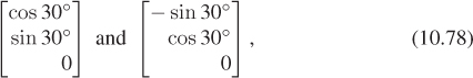
respectively. In this case, instead of finding matrices that send the vectors e1, e2, and e3 to the desired three points, before and after, we find matrices that send those vectors to the desired point and two vectors, before and after. These matrices are
so the overall matrix is
These general techniques can be applied to create any linear-plus-translation transformation of the w = 1 plane, but there are some specific ones that are good to know. Rotation in the xy-plane, by an amount θ (rotating the positive x-axis toward the positive y-axis) is given by
In some books and software packages, this is called rotation around z; we prefer the term “rotation in the xy-plane” because it also indicates the direction of rotation (from x, toward y). The other two standard rotations are
and
note that the last expression rotates z toward x, and not the opposite. Using this naming convention helps keep the pattern of plusses and minuses symmetric.
10.10. Coordinate Frames
In 2D, a linear transformation is completely specified by its values on two independent vectors. An affine transformation (i.e., linear plus translation) is completely specified by its values on any three noncollinear points, or on any point and pair of independent vectors. A projective transformation on the plane (which we’ll discuss briefly in Section 10.13) is specified by its values on four points, no three collinear, or on other possible sets of points and vectors. These facts, and the corresponding ones for transformations on 3-space, are so important that we enshrine them in a principle:
![]() The Transformation Uniqueness Principle
The Transformation Uniqueness Principle
For each class of transformations—linear, affine, and projective—and any corresponding coordinate frame, and any set of corresponding target elements, there’s a unique transformation mapping the frame elements to the correponding elements in the target frame. If the target elements themselves constitute a frame, then the transformation is invertible.
To make sense of this, we need to define a coordinate frame. As a first example, a coordinate frame for linear transformations is just a “basis”: In two dimensions, that means “two linearly independent vectors in the plane.” The elements of the frame are the two vectors. So the principle says that if u and v are linearly independent vectors in the plane, and u′ and v′ are any two vectors, then there’s a unique linear transformation sending u to u′ and v to v′. It further says that if u′ and v′ are independent, then the transformation is invertible.
More generally, a coordinate frame is a set of geometric elements rich enough to uniquely characterize a transformation in some class. For linear transformations of the plane, a coordinate frame consists of two independent vectors in the plane, as we said; for affine transforms of the plane, it consists of three noncollinear points in the plane, or of one point and two independent vectors, etc.
In cases where there are multiple kinds of coordinate frames, there’s always a way to convert between them. For 2D affine transformations, the three noncollinear points P, Q, and R can be converted to P, v1 = Q – P, and v2 = R – P; the conversion in the other direction is obvious. (It may not be obvious that the vectors v1 and v2 are linearly independent. See Exercise 10.4.)
There’s a restricted use of “coordinate frame” for affine maps that has some advantages. Based on the notion that the origin and the unit vectors along the positive directions for each axis form a frame, we’ll say that a rigid coordinate frame for the plane is a triple (P, v1, v2), where P is a point and v1 and v2 are perpendicular unit vectors with the rotation from v1 toward v2 being counterclockwise (i.e., with ![]() ). The corresponding definition for 3-space has one point and three mutually perpendicular unit vectors forming a right-hand coordinate system. Transforming one rigid coordinate frame (P, v1, v2) to another (Q, u1, u2) can always be effected by a sequence of transformation,
). The corresponding definition for 3-space has one point and three mutually perpendicular unit vectors forming a right-hand coordinate system. Transforming one rigid coordinate frame (P, v1, v2) to another (Q, u1, u2) can always be effected by a sequence of transformation,
where TP(A) = A + P is translation by P, and similarly for TQ, and R is the rotation given by
where the semicolon indicates that u1 is the first column of the first factor, etc.
The G3D library, which we use in examples in Chapters 12, 15, and 32, uses rigid coordinate frames extensively in modeling, encapsulating them in a class, CFrame.
10.11. Application: Rendering from a Scene Graph
We’ve discussed affine transformations on a two-dimensional affine space, and how, once we have a coordinate system and can represent points as triples, as in X = [x y 1]1, we can represent a transformation by a 3 × 3 matrix M. We transform the point x by multiplying it on the left by M to get Mx. With this in mind, let’s return to the clock example of Chapter 2 and ask how we could start from a WPF description and convert it to an image, that is, how we’d do some of the work that WPF does. You’ll recall that the clock shown in Figure 10.16 was created in WPF with code like this,
1 <Canvas ... >
2 <Ellipse
3 Canvas.Left="-10.0" Canvas.Top="-10.0"
4 Width="20.0" Height="20.0"
5 Fill="lightgray" />
6 <Control Name="Hour Hand" .../>
7 <Control Name="Minute Hand" .../>
8 <Canvas.RenderTransform>
9 <TransformGroup>
10 <ScaleTransform ScaleX="4.8" ScaleY="4.8" />
11 <TranslateTransform X="48" Y="48" />
12 </TransformGroup>
13 </Canvas.RenderTransform>
14 </Canvas>

where the code for the hour hand is
1 <Control Name="HourHand" Template="{StaticResource ClockHandTemplate}">
2 <Control.RenderTransform>
3 <TransformGroup>
4 <ScaleTransform ScaleX="1.7" ScaleY="0.7" />
5 <RotateTransform Angle="180"/>
6 <RotateTransform x:Name="ActualTimeHour" Angle="0"/>
7 </TransformGroup>
8 </Control.RenderTransform>
9 </Control>
and the code for the minute hand is similar, the only differences being that ActualTimeHour is replaced by ActualTimeMinute and the scale by 1.7 in X and 0.7 in Y is omitted.
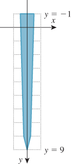
The ClockHandTemplate was a polygon defined by five points in the plane: (–0. 3, –1), (–0.2, 8), (0, 9), (0.2, 8), and (0. 3, –1) (see Figure 10.17).
We’re going to slightly modify this code so that the clock face and clock hands are both described in the same way, as polygons. We could create a polygonal version of the circular face by making a regular polygon with, say, 1000 vertices, but to keep the code simple and readable, we’ll make an octagonal approximation of a circle instead.
Now the code begins like this:
1 <Canvas ...
2 <Canvas.Resources>
3 <ControlTemplate x:Key="ClockHandTemplate">
4 <Polygon
5 Points="-0.3,-1 -0.2,8 0,9 0.2,8 0.3,-1"
6 Fill="Navy"/>
7 </ControlTemplate>
8 <ControlTemplate x:Key="CircleTemplate">
9 <Polygon
10 Points="1,0 0.707,0.707 0,1 -.707,.707
11 -1,0 -.707,-.707 0,-1 0.707,-.707"
12 Fill="LightGray"/>
13 </ControlTemplate>
14 </Canvas.Resources>
This code defines the geometry that we’ll use to create the face and hands of the clock. With this change, the circular clock face will be defined by transforming a template “circle,” represented by eight evenly spaced points on the unit circle. This form of specification, although not idiomatic in WPF, is quite similar to scene specification in many other scene-graph packages.
The actual creation of the scene now includes building the clock face from the CircleTemplate, and building the hands as before.
1 <!- 1. Background of the clock ->
2 <Control Name="Face"
3 Template="{StaticResource CircleTemplate}">
4 <Control.RenderTransform>
5 <ScaleTransform ScaleX="10" ScaleY="10" />
6 </Control.RenderTransform>
7 </Control>
8
9 <!- 2. The minute hand ->
10 <Control Name="MinuteHand"
11 Template="{StaticResource ClockHandTemplate}">
12 <Control.RenderTransform>
13 <TransformGroup>
14 <RotateTransform Angle="180" />
15 <RotateTransform x:Name="ActualTimeMinute" Angle="0" />
16 </TransformGroup>
17 </Control.RenderTransform>
18 </Control>
19
20 <!- 3. The hour hand ->
21 <Control Name="HourHand" Template="{StaticResource ClockHandTemplate}">
22 <Control.RenderTransform>
23 <TransformGroup>
24 <ScaleTransform ScaleX="1.7" ScaleY="0.7" />
25 <RotateTransform Angle="180" />
26 <RotateTransform x:Name="ActualTimeHour"
27 Angle="0" />
28 </TransformGroup>
29 </Control.RenderTransform>
30 </Control>
All that remains is the transformation from Canvas to WPF coordinates, and the timers for the animation, which set the ActualTimeMinute and ActualTimeHour values.
1 <Canvas.RenderTransform>
2 ...same as before...
3 </Canvas.RenderTransform>
4
5 <Canvas.Triggers>
6 <EventTrigger RoutedEvent="FrameworkElement.Loaded">
7 <BeginStoryboard>
8 <Storyboard>
9 <DoubleAnimation
10 Storyboard.TargetName="ActualTimeHour"
11 Storyboard.TargetProperty="Angle"
12 From="0.0" To="360.0"
13 Duration="00:00:01:0" RepeatBehavior="Forever"
14 />
15 <DoubleAnimation
16 Storyboard.TargetName="ActualTimeMinute"
17 Storyboard.TargetProperty="Angle"
18 From="0.0" To="4320.0"
19 Duration="00:00:01:0" RepeatBehavior="Forever"
20 />
21 </Storyboard>
22 </BeginStoryboard>
23 </EventTrigger>
24 </Canvas.Triggers>
25
26 </Canvas>
As a starting point in transforming this scene description into an image, we’ll assume that we have a basic graphics library that, given an array of points representing a polygon, can draw that polygon. The points will be represented by a 3×k array of homogeneous coordinate triples, so the first column of the array will be the homogeneous coordinates of the first polygon point, etc.
We’ll now explain how we can go from something like the WPF description to a sequence of drawPolygon calls. First, let’s transform the XAML code into a tree structure, as shown in Figure 10.18, representing the scene graph (see Chapter 6).
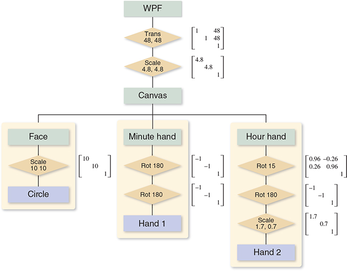
We’ve drawn transformations as diamonds, geometry as blue boxes, and named parts as beige boxes. For the moment, we’ve omitted the matter of instancing of the ClockHandTemplate and pretended that we have two separate identical copies of the geometry for a clock hand. We’ve also drawn next to each transformation the matrix representation of the transformation. We’ve assumed that the angle in ActualTimeHour is 15° (whose cosine and sine are approximately 0.96 and 0.26, respectively) and the angle in ActualTimeMinutes is 180° (i.e., the clock is showing 12:30).
(a) Remembering that rotations in WPF are specified in degrees and that they rotate objects in a clockwise direction, check that the matrix given for the rotation of the hour hand by 15° is correct.
(b) If you found that the matrix was wrong, recall that in WPF x increases to the right and y increases down. Does this change your answer? By the way, if you ran this program in WPF and debugged it and printed the matrix, you’d find the negative sign on the (2, 1) entry instead of the (1, 2) entry. That’s because WPF internally uses row vectors to represents points, and multiplies them by transformation matrices on the right.
The order of items in the tree is a little different from the textual order, but there’s a natural correspondence between the two. If you consider the hour hand and look at all transformations that occur in its associated render transform or in the render transform of anything containing it (i.e., the whole clock), those are exactly the transforms you encounter as you read from the leaf node corresponding to the hour hand up toward the root node.
Write down all transformations applied to the circle template that’s used as the clock face by reading the XAML program. Confirm that they’re the same ones you get by reading upward from the “Circle” box in Figure 10.18.
In the scene graph we’ve drawn, the transformation matrices are the most important elements. We’re now going to discuss how these matrices and the coordinates of the points in the geometry nodes interact.
Recall that there are two ways to think about transformations. The first is to say that the minute hand, for instance, has a rotation operation applied to each of its points, creating a new minute hand, which in turn has a translation applied to each point, creating yet another new minute hand, etc. The tip of the minute hand is at location (0, 9), once and for all. The tip of the rotated minute hand is somewhere else, and the tip of the translated and rotated minute hand is somewhere else again. It’s common to talk about all of these as if they were the same thing (“Now the tip of the minute hand is at (3, 17)...”), but that doesn’t really make sense—the tip of the minute hand cannot be in two different places.
The second view says that there are several different coordinate systems, and that the transformations tell you how to get from the tip’s coordinates in one system to its coordinates in another. We can then say things like, “The tip of the minute hand is at (0, 9) in object space or object coordinates, but it’s at (0, –9) in canvas coordinates.” Of course, the position in canvas coordinates depends on the amount by which the tip of the minute hand is rotated (we’ve assumed that the ActualTimeMinute rotation is 180°, so it has just undergone two 180° rotations). Similarly, the WPF coordinates for the tip of the minute hand are computed by further scaling each canvas coordinate by 4.8, and then adding 48 to each, resulting in WPF coordinates of (48, 4.8).
For this example, we have seven coordinate systems, most indicated by pale green boxes. Starting at the top, there are WPF coordinates, the coordinates used by drawPolygon(). It’s possible that internally, drawPolygon() must convert to, say, pixel coordinates, but this conversion is hidden from us, and we won’t discuss it further. Beneath the WPF coordinates are canvas coordinates, and within the canvas are the clock-face coordinates, minute-hand coordinates, and hour-hand coordinates. Below this are the hand coordinates, the coordinate system in which the single prototype hand was created, and circle coordinates, in which the prototype octagonal circle approximation was created. Notice that in our model of the clock, the clock-face, minute-hand, and hour-hand coordinates all play similar roles: In the hierarchy of coordinate systems, they’re all children of the canvas coordinate system. It might also have been reasonable to make the minute-hand and hour-hand coordinate systems children of the clock-face coordinate system. The advantage of doing so would have been that translating the clock face would have translated the whole clock, making it easier to adjust the clock’s position on the canvas. Right now, adjusting the clock’s position on the canvas requires that we adjust three different translations, which we’d have to add to the face, the minute hand, and the hour hand.
We’re hoping to draw each shape with a drawPolygon() call, which takes an array of point coordinates as an argument. For this to make sense, we have to declare the coordinate system in which the point coordinates are valid. We’ll assume that drawPolygon() expects WPF coordinates. So when we want to tell it about the tip of the minute hand, we’ll need the numbers (48, 4.8) rather than (0, 9).
Here’s a strawman algorithm for converting a scene graph into a sequence of drawPolygon() calls. We’ll work with 3×k arrays of coordinates, because we’ll represent the point (0, 9) as a homogeneous triple (0, 9, 1), which we’ll write vertically as a column of the matrix that represents the geometry.
1 for each polygonal geometry element, g
2 let v be the 3 × k array of vertices of g
3 let n be the parent node of g
4 let M be the 3 × 3 identity matrix
5 while (n is not the root)
6 if n is a transformation with matrix S
7 M = SM
8 n = parent of n
9
10 w = Mv
11 drawPolygon(w)
As you can see, we multiply together several matrices, and then multiply the result (the composite transformation matrix) by the vertex coordinates to get the WPF coordinates for each polygon, which we then draw.
(a) How many elementary operations are needed, approximately, to multiply a 3 × 3 matrix by a 3 × k matrix?
(b) If A and B are 3×3 and C is 3×1000, would you rather compute (AB)C or A(BC), where the parentheses are meant to indicate the order of calculations that you perform?
(c) In the code above, should we have multiplied the vertex coordinates by each matrix in turn, or was it wiser to accumulate the matrix product and only multiply by the vertex array at the end? Why?
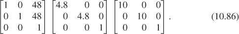
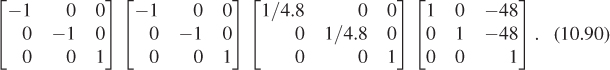
If we hand-simulate the code in the clock example, the circle template coordinates are multiplied by the matrix
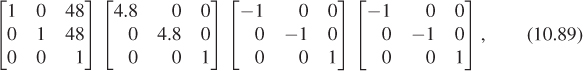
The minute-hand template coordinates are multiplied by the matrix

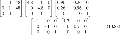
And the hour-hand template coordinates are multiplied by the matrix
Notice how much of this matrix multiplication is shared. We could have computed the product for the circle and reused it in each of the others, for instance. For a large scene graph, the overlap is often much greater. If there are 70 transformations applied to an object with only five or six vertices, the cost of multiplying matrices together far outweighs the cost of multiplying the composite matrix by the vertex coordinate array.
We can avoid duplicated work by revising our strawman algorithm. We perform a depth-first traversal of the scene graph, maintaining a stack of matrices as we do so. Each time we encounter a new transformation with matrix M, we multiply M by the current transformation matrix C (the one at the top of the stack) and push the result, MC, onto the stack. Each time our traversal rises up through a transformation node, we pop a matrix from the stack. The result is that whenever we encounter geometry (like the coordinates of the hand points, or of the ellipse points), we can multiply the coordinate array on the left by the current transformation to get the WPF coordinates of those points. In the pseudocode below, we assume that the scene graph is represented by a Scene class with a method that returns the root node of the graph, and that a transformation node has a matrix method that returns the matrix for the associated transformation, while a geometry node has a vertexCoordinateArray method that returns a 3 × k array containing the homogeneous coordinates of the k points in the polygon.
1 void drawScene(Scene myScene)
2 s = empty Stack
3 s.push( 3 × 3 identity matrix )
4 explore(myScene.rootNode(), s)
5
6
7 void explore(Node n, Stack& s)
8 if n is a transformation node
9 push n.matrix() * s.top() onto s
10
11 else if n is a geometry node
12 drawPolygon(s.top() * n.vertexCoordinateArray())
13
14 foreach child k of n
15 explore(k, s)
16
17 if n is a transformation node
18 pop top element from s
In some complex models, the cost of matrix multiplications can be enormous. If the same model is to be rendered over and over, and none of the transformations change (e.g., a model of a building in a driving-simulation game), it’s often worth it to use the algorithm above to create a list of polygons in world coordinates that can be redrawn for each frame, rather than reparsing the scene once per frame. This is sometimes referred to as prebaking or baking a model.
The algorithm above is the core of the standard one used for scene traversals in scene graphs. There are two important additions, however.
First, geometric transformations are not the only things stored in a scene graph—in some cases, attributes like color may be stored as well. In a simple version, each geometry node has a color, and the drawPolygon procedure is passed both the vertex coordinate array and the color. In a more complex version, the color attribute may be set at some node in the graph, and that color is used for all the geometry “beneath” that node. In this latter form, we can keep track of the color with a parallel stack onto which colors are pushed as they’re encountered, just as transformations are pushed onto the transformation stack. The difference is that while transformations are multiplied by the previous composite transformation before being pushed on the stack, the colors, representing an absolute rather than a relative attribute, are pushed without being combined in any way with previous color settings. It’s easy to imagine a scene graph in which color-alteration nodes are allowed (e.g., “Lighten everything below this node by 20%”); in such a structure, the stack would have to accumulate color transformations. Unless the transformations are quite limited, there’s no obvious way to combine them except to treat them as a sequence of transformations; matrix transformations are rather special in this regard.
Second, we’ve studied an example in which the scene graph is a tree, but depth-first traversal actually makes sense in an arbitrary directed acyclic graph (DAG). And in fact, our clock model, in reality, is a DAG: The geometry for the two clock hands is shared by the hands (using a WPF StaticResource). During the depth-first traversal we arrive at the hand geometry twice, and thus render two different hands. For a more complex model (e.g., a scene full of identical robots) such repeated encounters with the same geometry may be very frequent: Each robot has two identical arms that refer to the same underlying arm model; each arm has three identical fingers that refer to the same underlying finger model, etc. It’s clear that in such a situation, there’s some lost effort in retraversal of the arm model. Doing some analysis of a scene graph to detect such retraversals and avoid them by prebaking can be a useful optimization, although in many of today’s graphics applications, scene traversal is only a tiny fraction of the cost, and lighting and shading computations (for 3D models) dominate. You should avoid optimizing the scene-traversal portions of your code until you’ve verified that they are the expensive part.
10.11.1. Coordinate Changes in Scene Graphs
Returning to the scene graph and the matrix products, the transformations applied to the minute hand to get WPF coordinates,
represent the transformation from minute-hand coordinates to WPF coordinates. To go from WPF coordinates to minute-hand coordinates, we need only apply the inverse transformation. Remembering that (AB)–1 = B–1A–1, this inverse transformation is
You can similarly find the coordinate transformation matrix to get from any one coordinate system in a scene graph to any other. Reading upward, you accumulate the matrices you encounter, with the first matrix being farthest to the right; reading downward, you accumulate their inverses in the opposite order. When we build scene graphs in 3D, exactly the same rules apply.
For a 3D scene, there’s the description not only of the model, but also of how to transform points of the model into points on the display. This latter description is provided by specifying a camera. But even in 2D, there’s something closely analogous: The Canvas in which we created our clock model corresponds to the “world” of a 3D scene; the way that we transform this world to make it appear on the display (scale by (4.8, 4.8) and then translate by (48, 48)) corresponds to the viewing transformation performed by a 3D camera.
Typically the polygon coordinates (the ones we’ve placed in templates) are called modeling coordinates. Given the analogy to 3D, we can call the canvas coordinates world coordinates, while the WPF coordinates can be called image coordinates. These terms are all in common use when discussing 3D scene graphs.
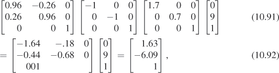
As an exercise, let’s consider the tip of the hour hand; in modeling coordinates (i.e., in the clock-hand template) the tip is located at (0, 9). In the same way, the tip of the minute hand, in modeling coordinates, is at (0, 9). What are the Canvas coordinates of the tip of the hour hand? We must multiply (reading from leaf toward root) by all the transformation matrices from the hour-hand template up to the Canvas, resulting in
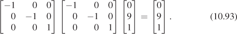
where all coordinates have been rounded to two decimal places for clarity. The Canvas coordinates of the tip of the minute hand are
We can thus compute a vector from the hour hand’s tip to the minute hand’s tip by subtracting these two, getting [–1.63 15.08 0]T. The result is the homogeneous-coordinate representation of the vector [–1.63 15.08]T in Canvas coordinates.
Suppose that we wanted to know the direction from the tip of the minute hand to the tip of the hour hand in minute-hand coordinates. If we knew this direction, we could add, within the minute-hand part of the model, a small arrow that pointed toward the hour-hand. To find this direction vector, we need to know the coordinates of the tip of the hour hand in minute-hand coordinates. So we must go from hour-hand coordinates to minute-hand coordinates, which we can do by working up the tree from the hour hand to the Canvas, and then back down to the minute hand. The location of the hour-hand tip, in minute-hand coordinates, is given by
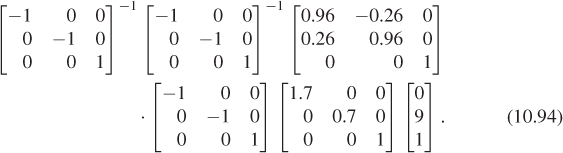
We subtract from this the coordinates, (0, 9), of the tip of the minute hand (in the minute-hand coordinate system) to get a vector from the tip of the minute hand to the tip of the hour hand.
As a final exercise, suppose we wanted to create an animation of the clock in which someone has grabbed the minute hand and held it so that the rest of the clock spins around the minute hand. How could we do this?
Well, the reason the minute hand moves from its initial 12:00 position on the Canvas (i.e., its position after it has been rotated 180° the first time) is that a sequence of further transformations have been applied to it. This sequence is rather short: It’s just the varying rotation. If we apply the inverse of this varying rotation to each of the clock elements, we’ll get the desired result. Because we apply both the rotation and its inverse to the minute hand, we could delete both, but the structure is more readable if we retain them. We could also apply the inverse rotation as part of the Canvas’s render transform.
If we want to implement the second approach—inserting the inverse rotation in the Canvas’s render transform—should it appear (in the WPF code) before or after the scale-and-translate transforms that are already there? Try it!
10.12. Transforming Vectors and Covectors
We’ve agreed to say that the point (x, y) ![]() E2 corresponds to the 3-space vector [x y 1]T, and that the vector
E2 corresponds to the 3-space vector [x y 1]T, and that the vector ![]() corresponds to the 3-space vector [u v 0]T. If we use a 3 × 3 matrix M (with last row [0 0 1]) to transform 3-space via
corresponds to the 3-space vector [u v 0]T. If we use a 3 × 3 matrix M (with last row [0 0 1]) to transform 3-space via
then the restriction of T to the w = 1 plane has its image in E2 as well, so we can write
But we also noted above that we could regard T as transforming vectors, or displacements of two-dimensional Euclidean space, which are typically written with two coordinates but which we represent in the form [u v 0]T. Because the last entry of such a “vector” is always 0, the last column of M has no effect on how vectors are transformed. Instead of computing
we could equally well compute
and the result would have a 0 in the third place. In fact, we could transform such vectors directly as two-coordinate vectors, by simply computing
For this reason, it’s sometimes said for an affine transformation of the Euclidean plane represented by multiplication by a matrix M that the associated transformation of vectors is represented by
What about covectors? Recall that a typical covector could be written in the form
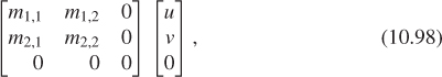
where w was some vector in R2. We’d like to transform φw in a way that’s consistent with T. Figure 10.19 shows why: We often build a geometric model of some shape and compute all the normal vectors to the shape. Suppose that n is one such surface normal. We then place that shape into 3-space by applying some “modeling transformation” TM to it, and we’d like to know the normal vectors to that transformed shape so that we can do things like compute the angle between a light-ray v and that surface normal. If we call the transformed surface normal m, we want to compute v · m. How is m related to the surface normal n of the original model?
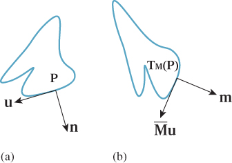
Figure 10.19: (a) A geometric shape that’s been modeled using some modeling tool; the normal vector n at a particular point P has been computed too. The vector u is tangent to the shape at P. (b) The shape has been translated, rotated, and scaled as it was placed into a scene. At the transformed location of P, we want to find the normal vector m with the property that its inner product with the transformed tangent ![]() u is still 0.
u is still 0.
The original surface normal n was defined by the property that it was orthogonal to every vector u that was tangent to the surface. The new normal vector m must be orthogonal to all the transformed tangent vectors, which are tangent to the transformed surface. In other words, we need to have
for every tangent vector u to the surface. In fact, we can go further. For any vector u, we’d like to have
that is, we’d like to be sure that the angle between an untransformed vector and n is the same as the angle between a transformed vector and m.
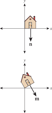
Before working through this, let’s look at a couple of examples. In the case of the transformation T1, the vector perpendicular to the bottom side of the house (we’ll use this as our vector n) should be transformed so that it’s still perpendicular to the bottom of the transformed house. This is achieved by rotating it by 30° (see Figure 10.20).
If we just translate the house, then n again should be transformed just the way we transform ordinary vectors, that is, not at all.
But what about when we shear the house, as with example transformation T3? The associated vector transformation is still a shearing transformation; it takes a vertical vector and tilts it! But the vector n, if it’s to remain perpendicular to the bottom of the house, must not be changed at all (see Figure 10.21). So, in this case, we see the necessity of transforming covectors differently from vectors.
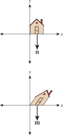
Figure 10.21: While the vertical sides of the house are sheared, the normal vector to the house’s bottom remains unchanged.
Let’s write down, once again, what we want. We’re looking for a vector m that satisfies
for every possible vector u. To make the algebra more obvious, let’s swap the order of the vectors and say that we want
Recalling that a · b can be written aTb, we can rewrite this as
Remembering that (AB)T = ATBT, and then simplifying, we get
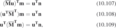
where the last step follows from the associativity of matrix multiplication. This last equality is of the form u · a = u · b for all u. Such an equality holds if and only if a = b, that is, if and only if
where we are assuming that ![]() is invertible.
is invertible.
We can therefore conclude that the covector φn transforms to the covector ![]() . For this reason, the inverse transpose is sometimes referred to as the covector transformation or (because of its frequent application to normal vectors) the normal transform. Note that if we choose to write covectors as row vectors, then the transpose is not needed, but we have to multiply the row vector on the right by
. For this reason, the inverse transpose is sometimes referred to as the covector transformation or (because of its frequent application to normal vectors) the normal transform. Note that if we choose to write covectors as row vectors, then the transpose is not needed, but we have to multiply the row vector on the right by ![]() .
.
![]() The normal transform, in its natural mathematical setting, goes in the opposite direction: It takes a normal vector in the codomain of TM and produces one in the domain; the matrix for this adjoint transformation is MT. Because we need to use it in the other direction, we end up with an inverse as well.
The normal transform, in its natural mathematical setting, goes in the opposite direction: It takes a normal vector in the codomain of TM and produces one in the domain; the matrix for this adjoint transformation is MT. Because we need to use it in the other direction, we end up with an inverse as well.
Taking our shearing transformation, T3, as an example, when written in xyw-space the matrix M for the transformation is
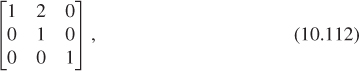
and hence ![]() is
is
while the normal transform is
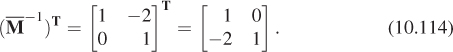
Hence the covector φn, where ![]() , for example, becomes the covector φm,
, for example, becomes the covector φm,
where ![]() .
.
(a) Find an equation (in coordinates, not vector form) for a line passing through the point P = (1, 1), with normal vector ![]() .
.
(b) Find a second point Q on this line. (c) Find P′ = T3(P) and Q′ = T3(Q), and a coordinate equation of the line joining P′ and Q′. (d) Verify that the normal to this second line is in fact proportional to ![]() , confirming that the normal transform really did properly transform the normal vector to this line.
, confirming that the normal transform really did properly transform the normal vector to this line.
We assumed that the matrix M was invertible when we computed the normal transform. Give an intuitive explanation of why, if M is degenerate (i.e., not invertible), it’s impossible to define a normal transform. Hint: Suppose that u, in the discussion above, is sent to 0 by M, but that u · n is nonzero.
10.12.1. Transforming Parametric Lines
All the transformations of the w = 1 plane we’ve looked at share the property that they send lines into lines. But more than that is true: They send parametric lines to parametric lines, by which we mean that if ![]() is the parametric line
is the parametric line ![]() = {P + t v : t εR}, and Q = P + v (i.e.,
= {P + t v : t εR}, and Q = P + v (i.e., ![]() starts at P and reaches Q at t = 1), and T is the transformation T(v) = Mv, then T(
starts at P and reaches Q at t = 1), and T is the transformation T(v) = Mv, then T(![]() ) is the line
) is the line
and in fact, the point at parameter t in ![]() (namely P + t(Q – P)) is sent by T to the point at parameter t in T(
(namely P + t(Q – P)) is sent by T to the point at parameter t in T(![]() ) (namely T(P) + t(T(Q) – T(P))).
) (namely T(P) + t(T(Q) – T(P))).
This means that for the transformations we’ve considered so far, transforming the plane commutes with forming affine or linear combinations, so you can either transform and then average a set of points, or average and then transform, for instance.
10.13. More General Transformations
Let’s look at one final transform, T, which is a prototype for transforms we’ll use when we study projections and cameras in 3D. All the essential ideas occur in 2D, so we’ll look at this transformation carefully. The matrix M for the transformation T is
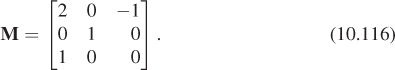
It’s easy to see that TM doesn’t transform the w = 1 plane into the w = 1 plane.
Figure 10.22 shows the w = 1 plane in blue and the transformed w = 1 plane in gray. To make the transformation T useful to us in our study of the w = 1 plane, we need to take the points of the gray plane and “return” them to the blue plane somehow. To do so, we introduce a new function, H, defined by
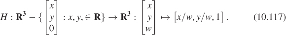
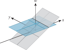
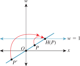
Figure 10.23 show how the analogous function in two dimensions sends every point except those on the w = 0 line to the line w = 1: For a typical point P, we connect P to the origin O with a line and see where this line meets the w = 1 line. Notice that even a point in the negative-w half-space on the same line gets sent to the same location on the w = 1 line. This connect-and-intersect operation isn’t defined, of course, for points on the x-axis, because the line connecting them to the origin is the axis itself, which never meets the w = 1 line. H is often called homogenization in graphics.
With H in hand, we’ll define a new transformation on the w = 1 plane by
This definition has a serious problem: As you can see from Figure 10.22, some points in the image of T are in the w = 0 plane, on which H is not defined so that S cannot be defined there. For now, we’ll ignore this and simply not apply S to any such points.
Find all points v = [x y 1]T of the w = 1 plane such that the w-coordinate of TM(v) is 0. These are the points on which S is undefined.
The transformation S, defined by multiplication by the matrix M, followed by homogenization, is called a projective transformation. Notice that if we followed either a linear or affine transformation with homogenization, the homogenization would have no effect. Thus, we have three nested classes of transformations: linear, affine (which includes linear and translation and combinations of them), and projective (which includes affine and transformations like S).
Figure 10.24 shows several objects in the w = 1 plane, drawn as seen looking down the w-axis, with the y-axis, on which S is undefined, shown in pale green. Figure 10.25 shows these objects after S has been applied to them. Evidently, S takes lines to lines, mostly: A line segment like the blue one in the figure that meets the y-axis in the segment’s interior turns into two rays, but the two rays both lie in the same line. We say that the line y = 0 has been “sent to infinity.” The red vertical line at x = 1 in Figure 10.24 transforms into the red vertical line at x = 0 in Figure 10.25. And every ray through the origin in Figure 10.24 turns into a horizontal line in Figure 10.25. We can say even more: Suppose that P1 denotes projection from the origin onto the x = 1 line in Figure 10.24, while P2 denotes horizontal projection onto the x = 0 line in Figure 10.25. Then
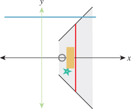
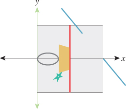
for any point X that’s not on the y-axis. In other words, S converts radial projection into parallel projection. In Chapter 13 we’ll see exactly the same trick in 3-space: We’ll convert radial projection toward the eye into parallel projection. This is useful because in parallel projection, it’s really easy to tell when one object obscures another by just comparing “depth” values!
Let’s look at how S transforms a parameterized line. Consider the line ![]() starting at a point P and passing through a point Q when t = 1,
starting at a point P and passing through a point Q when t = 1,
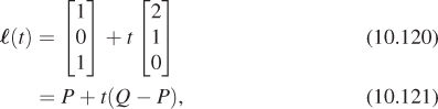
where P = [1 0 1]T and Q = [3 1 1]T so that in the w = 1 plane, the line starts at (x, y) = (1, 0) when t = 0 and goes to the right and slightly upward, arriving at (x, y) = (3, 1) when t = 1 (see Figure 10.26).
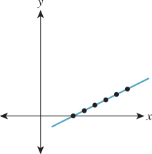
Figure 10.26: The line ![]() passes through P at t = 0 and Q at t = 1; the black points are equispaced in the interval 0 ≤ t ≤ 1.
passes through P at t = 0 and Q at t = 1; the black points are equispaced in the interval 0 ≤ t ≤ 1.
The function T transforms this to the line ![]() ′ that starts at T(P) = [1 0 1]T when t = 0 and arrives at T(Q) = [5 1 3]T when t = 1, and whose equation is
′ that starts at T(P) = [1 0 1]T when t = 0 and arrives at T(Q) = [5 1 3]T when t = 1, and whose equation is
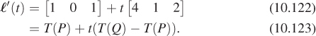
Figure 10.27 shows the line in 3-space, after transformation by TM; the point spacing remains constant.
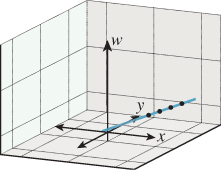
We know that this is the parametric equation of the line, because every linear transformation transforms parametric lines to parametric lines. But when we apply H, something interesting happens. Because the function H is not linear, the parametric line is not transformed to a parametric line. The point ![]() ′ (t) = [1 + 4t t 1 + 2t]T is sent to
′ (t) = [1 + 4t t 1 + 2t]T is sent to
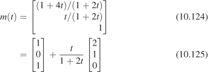
Equation 10.125 has almost the form of a parametric line, but the coefficient of the direction vector, which is proportional to S(Q) – S(P), has the form
which is called a fractional linear transformation of t. This nonstandard form is of serious importance in practice: It tells us that if we interpolate a value at the midpoint M of P and Q, for instance, from the values at P and Q, and then transform all three points by S, then S(M) will generally not be at the midpoint of S(P) and S(Q), so the interpolated value will not be the correct one to use if we need post-transformation interpolation. Figure 10.28 shows how the equally spaced points in the domain have become unevenly spaced after the projective transformation.
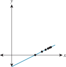
In other words, transformation by S and interpolation are not commuting operations. When we apply a transformation that includes the homogenization operation H, we cannot assume that interpolation will give the same results pre- and post-transformation. Fortunately, there’s a solution to this problem (see Section 15.6.4).
(a) Show that if n and f are distinct nonzero numbers, the transformation defined by the matrix
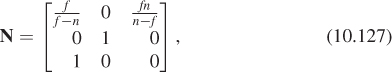
when followed by homogenization, sends the line x = 0 to infinity, the line x = n to x = 0, and the line x = f to x = 1.
(b) Figure out how to modify the matrix to send x = f to x = –1 instead.
(a) Show that if T is any linear transformation on R3, then for any nonzero α ![]() R and any vector v
R and any vector v ![]() R3, H(T(αv)) = H(T(v)). (b) Show that if K is any matrix, then H(TK(v)) = H(TαK(v)) as well. (c) Conclude that in a sequence of matrix operations in which there’s an H at the end, matrix scale doesn’t matter, that is, you can multiply a matrix by any nonzero constant without changing the end result.
R3, H(T(αv)) = H(T(v)). (b) Show that if K is any matrix, then H(TK(v)) = H(TαK(v)) as well. (c) Conclude that in a sequence of matrix operations in which there’s an H at the end, matrix scale doesn’t matter, that is, you can multiply a matrix by any nonzero constant without changing the end result.
Suppose we have a matrix transformation on 3-space given by T(v) = Kv, and T is nondegenerate (i.e., T(v) = 0 only when v = 0). Then T takes lines through the origin to lines through the origin, because if v = 0 is any nonzero vector, then {α v : α ![]() R} is the line through the origin containing v, and when we transform this, we get {αT(v) : α
R} is the line through the origin containing v, and when we transform this, we get {αT(v) : α ![]() R}, which is the line through the origin containing T(v). Thus, rather than thinking of the transformation T as moving around points in R3, we can think of it as acting on the set of lines through the origin. By intersecting each line through the origin with the w = 1 plane, we can regard T as acting on the w = 1 plane, but with a slight problem: A line through the origin in 3-space that meets the w = 1 plane may be transformed to one that does not (i.e., a horizontal line), and vice versa. So using the w = 1 plane to “understand” the lines-to-lines version of the transformation T is a little confusing.
R}, which is the line through the origin containing T(v). Thus, rather than thinking of the transformation T as moving around points in R3, we can think of it as acting on the set of lines through the origin. By intersecting each line through the origin with the w = 1 plane, we can regard T as acting on the w = 1 plane, but with a slight problem: A line through the origin in 3-space that meets the w = 1 plane may be transformed to one that does not (i.e., a horizontal line), and vice versa. So using the w = 1 plane to “understand” the lines-to-lines version of the transformation T is a little confusing.
The idea of considering linear transformations as transformations on the set of lines through the origin is central to the field of projective geometry. An understanding of projective geometry can lead to a deeper understanding of the transformations we use in graphics, but is by no means essential. Hartshorne [Har09] provides an excellent introduction for the student who has studied abstract algebra.
Transformations of the w = 1 plane like the ones we’ve been looking at in this section, consisting of an arbitrary matrix transformation on R3 followed by H, are called projective transformations. The class of projective transformations includes all the more basic operations like translation, rotation, and scaling of the plane (i.e., affine transformations of the plane), but include many others as well. Just as with linear and affine transformations, there’s a uniqueness theorem: If P, Q, R, and S are four points of the plane, no three collinear, then there’s exactly one projective transformation sending these points to (0, 0), (1, 0), (0, 1), and (1, 1), respectively. (Note that this one transformation might be described by two different matrices. For example, if K is the matrix of a projective transformation S, then 2K defines exactly the same transformation.)
For all the affine transformations we discussed in earlier sections, we’ve determined an associated transformation of vectors and of normal vectors. For projective transformations, this process is messier. Under the projective transformation shown in Figures 10.24 and 10.25, we can consider the top and bottom edges of the tan rectangle as vectors that point in the same direction. After the transformation, you can see that they have been transformed to point in different directions. There’s no single “vector” transformation to apply. If we have a vector v starting at the point P, we have to apply “the vector transformation at P” to v to find out where it will go. The same idea applies to normal vectors: There’s a different normal transformation at every point. In both cases, it’s the function H that leads to problems. The “vector” transformation for any function U is, in general, the derivative DU. In the case of a matrix transformation TM that’s being applied only to points of the w = 1 plane, the “vectors” lying in that plane all have w = 0, and so the matrix used to transform these vectors can have its third column set to be all zeroes (or can be just written as a 2 × 2 matrix operating on vectors with two entries), as we have seen earlier. But since
we have (using the multivariable chain rule)
Now, since 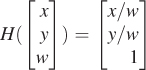 , we know that
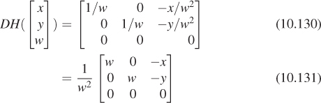
and
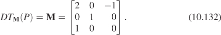
So, if P = [x, y, 1] is a point of the w = 1 plane and  is a vector in that plane, then
  and
and
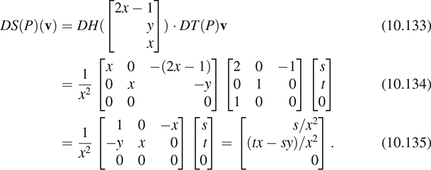
Evidently, the “vector” transformation depends on the point (x, y, 1) at which it’s applied. The normal transform, being the inverse transpose of the vector transform, has the same dependence on the point of application.
10.14. Transformations versus Interpolation
When you rotate a book on your desk by 30° counterclockwise, the book is rotated by each intermediate amount between zero and 30°. But when we “rotate” the house in our diagram by 30°, we simply compute the final position of each point of the house. In no sense has it passed through any intermediate positions. In the more extreme case of rotation by 180°, the resultant transformation is exactly the same as the “uniform scale by –1” transformation. And in the case of rotation by 360°, the resultant transformation is the identity.
This reflects a limitation in modeling. The use of matrix transformations to model transformations of ordinary objects captures only the relationship between initial and final positions, and not the means by which the object got from the initial to the final position.
Much of the time, this distinction is unimportant: We want to put an object into a particular pose, so we apply some sequence of transformations to it (or its parts). But sometimes it can be quite significant: We might instead want to show the object being transformed from its initial state to its final state. An easy, but rarely useful, approach is to linearly interpolate each point of the object from its initial to its final position. If we do this for the “rotation by 180°” example, at the halfway point the entire object is collapsed to a single point; if we do it from the “rotation by 360°” example, the object never appears to move at all! The problem is that what we really want is to find interpolated versions of our descriptions of the transformation rather than of the transformations themselves. (Thus, to go from the initial state to “rotated by 360” we’d apply “rotate by s” to the initial state, for each value of s from 0 to 360.)
But sometimes students confuse a transformation like “multiplication by the identity matrix” with the way it was specified, “rotate by 360°,” and they can be frustrated with the impossibility of “dividing by two” to get a rotation by 180°, for instance. This is particularly annoying when one has access only to the matrix form of the transformation, rather than the initial specification; in that case, as the examples show, there’s no hope for a general solution to the problem of “doing a transformation partway.” On the other hand, there is a solution that often gives reasonable results in practice, especially for the problem of interpolating two rather similar transformations (e.g., interpolating between rotating by 20° and rotating by 30°), which often arises. We’ll discuss this in Chapter 11.
10.15. Discussion and Further Reading
We’ve introduced three classes of basic transformations: linear, which you’ve already encountered in linear algebra; affine, which includes translations and can be seen as a subset of the linear transformations in xyw-space, restricted to the w = 1 plane; and projective, which arises from general linear transformations on xyw-space, restricted to the w = 1 plane and then followed by the homogenization operation that divides through by w. We’ve shown how to represent each kind of transformation by matrix multiplication, but we urge you to separate the idea of a transformation from the matrix that represents it.
For each category, there’s a theorem about uniqueness: A linear transformation on the plane is determined by its values on two independent vectors; an affine transformation is determined by its values on any three noncollinear points; a projective transformation is determined by its values on any four points, no three of which are collinear. In the next chapter we’ll see analogous results for 3-space, and in the following one we’ll see how to use these theorems to build a library for representing transformations so that you don’t have to spend a lot of time building individual matrices.
Even though matrices are not as easy for humans to interpret as “This transformation sends the points A, B, and C to A′, B′, and C′,” the matrix representation of a transformation is very valuable, mostly because composition of transformation is equivalent to multiplication of matrices; performing a complex sequence of transformations on many points can be converted to multiplying the points’ coordinates by a single matrix.
10.16. Exercises
Exercise 10.1: Use the 2D test bed to write a program to demonstrate windowing transforms. The user should click and drag two rectangles, and you should compute the transform between them. Subsequent clicks by the user within the first rectangle should be shown as small dots, and the corresponding locations in the second rectangle should also be shown as dots. Provide a Clear button to let the user restart.
Exercise 10.2: Multiply ![]() by the expression given in Equation 10.17 for its inverse to verify that the product really is the identity.
by the expression given in Equation 10.17 for its inverse to verify that the product really is the identity.
Exercise 10.3: Suppose that M is an n × n square matrix with SVD M = UDVT.
(a) Why is VTV the identity?
(b) Let i be any number from 1 to n. What is VTvi, where vi denotes the ith column of V? Hint: Use part (a).
(c) What’s DVTvi?
(d) What’s Mvi in terms of ui and di, the ith diagonal entry of D?
(e) Let ![]() . Show that M′ vi = diui.
. Show that M′ vi = diui.
(f) Explain why vi, i = 1, ..., n are linearly independent, and thus span Rn.
(g) Conclude that w ![]() Mw and w
Mw and w ![]() M′ w agree on n linearly independent vectors, and hence must be the same linear transformation of Rn.
M′ w agree on n linearly independent vectors, and hence must be the same linear transformation of Rn.
(h) Conclude that M′ = M. Thus, the singular-value decomposition proves the theorem that every matrix can be written as a sum of outer products (i.e., matrices of the form vwT).
(a) If P, Q, and R are noncollinear points in the plane, show that Q – P and R – P are linearly independent vectors.
(b) If v1 and v2 are linearly independent points in the plane, and A is any point in the plane, show that A, B = A + v1 and C = A + v2 are noncollinear points. This shows that the two kinds of affine frames are equivalent.
(c) Two forms of an affine frame in 3-space are (i) four points, no three coplanar, and (ii) one point and three linearly independent vectors. Show how to convert from one to the other, and also describe a third possible version (Three points and one vector? Two points and two vectors? You choose!) and show its equivalence as well.
Exercise 10.5: We said that if the columns of the matrix M are v1, v2, ..., vk ![]() Rn, and they are pairwise orthogonal unit vectors, then MTM = Ik, the k × k identity matrix.
Rn, and they are pairwise orthogonal unit vectors, then MTM = Ik, the k × k identity matrix.
(a) Explain why, in this situation, k ≤ n.
(b) Prove the claim that MTM = Ik.
Exercise 10.6: An image (i.e., an array of grayscale values between 0 and 1, say) can be thought of as a large matrix, M (indeed, this is how we usually represent images in our programs). Use a linear algebra library to compute the SVD M = UDVT of some image M. According to the decomposition theorem described in Exercise 10.3, this describes the image as a sum of outer products of many vectors. If we replace the last 90% of the diagonal entries of D with zeroes to get a new matrix D′, then the product M′ = UD′ V deletes 90% of the terms in this sum of outer products. In doing so, however, it deletes the smallest 90% of the terms. Display M′ and compare it to M. Experiment with values other than 90%. At what level do the two images become indistinguishable? You may encounter values less than 0 and greater than 1 during the process described in this exercise. You should simply clamp these values to the interval [0, 1].
![]() Exercise 10.7: The rank of a matrix is the number of linearly independent columns of the matrix.
Exercise 10.7: The rank of a matrix is the number of linearly independent columns of the matrix.
(a) Explain why the outer product of two nonzero vectors always has rank one.
(b) The decomposition theorem described in Exercise 10.3 expresses a matrix M as a sum of rank one matrices. Explain why the sum of the first p such outer products has rank p (assuming d1, d2,..., dp ≠ 0). In fact, this sum Mp is the rank p matrix that’s closest to M, in the sense that the sum of the squares of the entries of M – Mp is as small as possible. (You need not prove this.)
Exercise 10.8: Suppose that T : R2 ![]() R2 is a linear transformation represented by the 2 × 2 matrix M, that is, T(x) = Mx. Let K = maxx
R2 is a linear transformation represented by the 2 × 2 matrix M, that is, T(x) = Mx. Let K = maxx![]() S1 ||T(X)||2, that is, K is the maximum squared length of all unit vectors transformed by M.
S1 ||T(X)||2, that is, K is the maximum squared length of all unit vectors transformed by M.
(a) If the SVD of M is M = UDVT, show that K = d21.
(b) What is the minimum squared length among all such vectors, in terms of D?
(c) Generalize to R3.
Exercise 10.9: Show that three distinct points P, Q, and R in the Euclidean plane are collinear if and only if the corresponding vectors ( , etc.) are linearly dependent, by showing that if αPvP + αQvQ + αRvR = 0 with not all the αs being 0, then
(a) none of the αs are 0, and
(b) the point Q is an affine combination of P and R; in particular, ![]() , so Q must lie on the line between P and R.
, so Q must lie on the line between P and R.
(c) Argue why dependence and collinearity are trivially the same if two or more of the points P, Q, and R are identical.
Exercise 10.10: It’s good to be able to recognize the transformation represented by a matrix by looking at the matrix; for instance, it’s easy to recognize a 3 × 3 matrix that represents a translation in homogeneous coordinates: Its last row is [0 0 1] and its upper-left 2 × 2 block is the identity. Given a 3 × 3 matrix representing a transformation in homogeneous coordinates,
(a) how can you tell whether the transformation is affine or not?
(b) How can you tell whether the transformation is linear or not?
(c) How can you tell whether it represents a rotation about the origin? (d) How can you tell if it represents a uniform scale?
Exercise 10.11: Suppose we have a linear transformation T : R2 ![]() R2, and two coordinate systems with bases {u1, u2} and {v1, v2}; all four basis vectors are unit vectors, u2 is 90° counterclockwise from u1, and similarly v2 is 90° counterclockwise from v1. You can write down the matrix Mu for T in the u-coordinate system and the matrix Mv for T in the v-coordinate system.
R2, and two coordinate systems with bases {u1, u2} and {v1, v2}; all four basis vectors are unit vectors, u2 is 90° counterclockwise from u1, and similarly v2 is 90° counterclockwise from v1. You can write down the matrix Mu for T in the u-coordinate system and the matrix Mv for T in the v-coordinate system.
(a) If Mu is a rotation matrix ![]() , what can you say about Mv?
, what can you say about Mv?
(b) If Mu is a uniform scaling matrix, that is, a multiple of the identity, what can you say about Mv?
(c) If Mu is a nonuniform scaling matrix of the form ![]() , with a ≠ b, what can you say about Mv?
, with a ≠ b, what can you say about Mv?