
Chapter 1. Introduction
This chapter introduces computer graphics quite broadly and from several perspectives: its applications, the various fields that are involved in the study of graphics, some of the tools that make the images produced by graphics so effective, some numbers to help you understand the scales at which computer graphics works, and the elementary ideas required to write your first graphics program. We’ll discuss many of these topics in more detail elsewhere in the book.
1.1. An Introduction to Computer Graphics
Computer graphics is the science and art of communicating visually via a computer’s display and its interaction devices. The visual aspect of the communication is usually in the computer-to-human direction, with the human-to-computer direction being mediated by devices like the mouse, keyboard, joystick, game controller, or touch-sensitive overlay. However, even this is beginning to change: Visual data is starting to flow back to the computer, with new interfaces being based on computer vision algorithms applied to video or depth-camera input. But for the computer-to-user direction, the ultimate consumers of the communications are human, and thus the ways that humans perceive imagery are critical in the design of graphics1 programs—features that humans ignore need not be presented (nor computed!). Computer graphics is a cross-disciplinary field in which physics, mathematics, human perception, human-computer interaction, engineering, graphic design, and art all play important roles. We use physics to model light and to perform simulations for animation. We use mathematics to describe shape. Human perceptual abilities determine our allocation of resources—we don’t want to spend time rendering things that will not be noticed. We use engineering in optimizing the allocation of bandwidth, memory, and processor time. Graphic design and art combine with human-computer interaction to make the computer-to-human direction of communication most effective. In this chapter, we discuss some application areas, how conventional graphics systems work, and how each of these disciplines influences work in computer graphics.
1. Throughout this book, when we use the term “graphics” we mean “computer graphics.”
A narrow definition of computer graphics would state that it refers to taking a model of the objects in a scene (a geometric description of the things in the scene and a description of how they reflect light) and a model of the light emitted into the scene (a mathematical description of the sources of light energy, the directions of radiation, the distribution of light wavelengths, etc.), and then producing a representation of a particular view of the scene (the light arriving at some imaginary eye or camera in the scene). In this view, one might say that graphics is just glorified multiplication: One multiplies the incoming light by the reflectivities of objects in the scene to compute the light leaving those objects’ surfaces and repeats the process (treating the surfaces as new light sources and recursively invoking the light-transport operation), determining all light that eventually reaches the camera. (In practice, this approach is unworkable, but the idea remains.) In contrast, computer vision amounts to factoring—given a view of a scene, the computer vision system is charged with determining the illumination and/or the scene’s contents (which a graphics system could then “multiply” together to reproduce the same image). In truth, of course, the vision system cannot solve the problem as stated and typically works with assumptions about the scene, or the lighting, or both, and may also have multiple views of the scene from different cameras, or multiple views from a single camera but at different times.
In actual fact, graphics is far richer than the generalized multiplication process of rendering a view, just as vision is richer than factorization. Much of the current research in graphics is in methods for creating geometric models, methods for representing surface reflectance (and subsurface reflectance, and reflectances of participating media such as fog and smoke, etc.), the animation of scenes by physical laws and by approximations of those laws, the control of animation, interaction with virtual objects, the invention of nonphotorealistic representations, and, in recent years, an increasing integration of techniques from computer vision. As a result, the fields of computer graphics and computer vision are growing increasingly closer to each other. For example, consider Raskar’s work on a nonphotorealistic camera: The camera takes multiple photos of a single scene, illuminated by differently placed flash units. From these various images, one can use computer vision techniques to determine contours and estimate some basic shape properties for objects in the scene. These, in turn, can be used to create a nonphotorealistic rendering of the scene, as shown in Figure 1.1.

Figure 1.1: A nonphotorealistic camera can create an artistic rendering of a scene by applying computer vision techniques to multiple flash-photo images and then rerendering the scene using computer graphics techniques. At left is the original scene; at right is the new rendering of the scene. (Courtesy of Ramesh Raskar; ©2004 ACM, Inc. Included here by permission.)
In this book, we emphasize realistic image capture and rendering because this is where the field of computer graphics has had the greatest successes, representing a beautiful application of relatively new computer science to the simulation of relatively old physics models. But there’s more to graphics than realistic image capture and rendering. Animation and interaction, for instance, are equally important, and we discuss these disciplines throughout many chapters in this book as well as address them explicitly in their own chapters. Why has success in the nonsimulation areas been so comparatively hard to achieve? Perhaps because these areas are more qualitative in nature and lack existing mathematical models like those provided by physics.
This book is not filled with recipes for implementing lots of ideas in computer graphics; instead, it provides a higher-level view of the subject, with the goal of teaching you ideas that will remain relevant long after particular implementations are no longer important. We believe that by synthesizing decades of research, we can elucidate principles that will help you in your study and use of computer graphics. You’ll generally need to write your own implementations or find them elsewhere.
This is not, by any means, because we disparage such information or the books that provide it. We admire such work and learn from it. And we admire those who can synthesize it into a coherent and well-presented whole. With this in mind, we strongly recommend that as you read this book, you keep a copy of Akenine-Möller, Haines, and Hoffman’s book on real-time rendering [AMHH08] next to you. An alternative, but less good, approach is to take any particular topic that interests you and search the Internet for information about it. The mathematician Abel claimed that he managed to succeed in mathematics because he made a practice of reading the works of the masters rather than their students, and we advise that you follow his lead. The aforementioned real-time rendering book is written by masters of the subject, while a random web page may be written by anyone. We believe that it’s far better, if you want to grab something from the Internet, to grab the original paper on the subject.
Having promised principles, we offer two right away, courtesy of Michael Littman:
![]() The Know Your Problem Principle
The Know Your Problem Principle
Know what problem you are solving.
![]() The Approximate the Solution Principle
The Approximate the Solution Principle
Approximate the solution, not the problem.
Both are good guides for research in general, but for graphics in particular, where there are so many widely used approximations that it’s sometimes easy to forget what the approximation is approximating, working with the unapproxi-mated entity may lead to a far clearer path to a solution to your problem.
1.1.1. The World of Computer Graphics
The academic side of computer graphics is dominated by SIGGRAPH, the Association for Computing Machinery’s Special Interest Group on Computer Graphics and Interactive Techniques; the annual SIGGRAPH conference is the premier venue for the presentation of new results in computer graphics, as well as a large commercial trade show and several colocated conferences in related areas. The SIGGRAPH proceedings, published by the ACM, are the most important reference works that a practitioner in the field can have. In recent years these have been published as an issue of the ACM Transactions on Graphics.
Computer graphics is also an industry, of course, and it has had an enormous impact in the areas of film, television, advertising, and games. It has also changed the way we look at information in medicine, architecture, industrial process control, network operations, and our day-to-day lives as we see weather maps and other information visualizations. Perhaps most significantly, the graphical user interfaces (GUIs) on our telephones, computers, automobile dashboards, and many home electronics devices are all enabled by computer graphics.
1.1.2. Current and Future Application Areas
Computer graphics has rapidly shifted from a novelty to an everyday phenomenon. Even throwaway devices, like the handheld digital games that parents give to children to keep them occupied on airplane trips, have graphical displays and interfaces. This corresponds to two phenomena: First visual perception is powerful, and visual communication is incredibly rapid, so designers of devices of all kinds want to use it, and second, the cost to manufacture computer-based devices is decreasing rapidly. (Roy Smith [Smi], discussing in the 1980s various claims that a GPS unit was so complex that it could never cost less than $1000, said, “Anything made of silicon will someday cost five dollars.” It’s a good rule of thumb.)
As graphics has become more prevalent, user expectations have risen. Video games display many millions of polygons per second, and special effects in films are now so good that they’re no longer readily distinguishable from non-computer-generated material. Digital cameras and digital video cameras give us huge streams of pixels (the individual items in an array of dots that constitutes the image2) to be processed, and the tools for processing them are rapidly evolving. At the same time, the increased power of computers has allowed the possibility of enriched forms of graphics. With the availability of digital photography, sophisticated scanners (Figure 1.2), and other tools, one no longer needs to explicitly create models of every object to be shown: Instead, one can scan the object directly, or even ignore the object altogether and use multiple digital images of it as a proxy for the thing itself. And with the enriched data streams, the possibility of extracting more and more information about the data—using techniques from computer vision, for instance—has begun to influence the possible applications of graphics. As an example, camera-based tracking technology lets body pose or gestures control games and other applications (Figure 1.3).
2. We’ll call these display pixels to distinguish them from other uses of the term “pixel,” which we’ll introduce in later chapters.
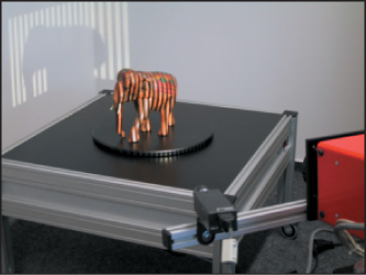
Figure 1.2: A scanner that projects stripes on a model that is slowly rotated on a turntable. The camera records the pattern of stripes in many positions to determine the object’s shape. (Courtesy of Polygon Technology, GMBH).
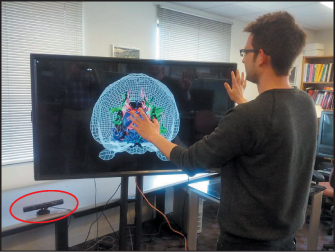
Figure 1.3: Microsoft’s Kinect interface can sense the user’s position and gestures, allowing a scientist to adjust the view of his data by “body language”, without a mouse or keyboard. (Data view courtesy of David Laid-law; image courtesy of Emanuel Zgraggen.)
While graphics has had an enormous impact on the entertainment industry, its influence in other areas—science, engineering (including computer-aided design and manufacturing), medicine, desktop publishing, website design, communication, information handling, and analysis are just a few examples—continues to grow daily. And new interaction settings ranging from large to small form factors—virtual reality, room-size displays (Figure 1.4), wearable displays containing twin LCDs in front of the user’s eyes, multitouch devices, including large-scale multitouch tables and walls (Figure 1.5), and smartphones—provide new opportunities for even greater impact.
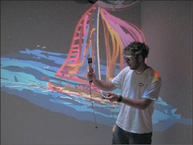
Figure 1.4: An artist stands in a Cave (a room whose walls are displays) and places paint strokes in 3D. The displays are synchronized with stereo glasses to display imagery so that it appears to float in midair in the room. Head-tracking technology allows the software to produce imagery that is correct for the user’s position and viewing direction, even as the user shifts his point of view. (Courtesy of Daniel Keefe, University of Minnesota).
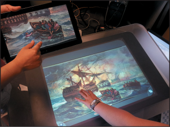
Figure 1.5: Two users interact with different portions of a large artwork on a large-scale touch-enabled display and a touch-enabled tablet display. (Courtesy of Brown Graphics Group.)
For most of the remainder of this chapter, when we speak about graphics applications we’ll have in mind applications such as video games, in which the most critical resources are the processor time, memory, and bandwidth associated with rendering—causing certain objects or images to appear on the display. There is, however, a wide range of application types, each with its own set of requirements and critical resources (see Section 1.11). A useful measure of performance to keep in mind, therefore, is primitives per second, where a primitive is some building block appropriate to the application; for an arcade-like video game it might be textured polygons, while for a fluid-flow-visualization system it might be short colored arrows. The number of primitives displayed per second is the product of the number of primitives displayed per frame (i.e., the displayed image) and the number of frames displayed per second. While some applications may choose to display more primitives per frame, to do so they will need to reduce their frame rates; others, aiming at smoothness in the animation, will want higher frame rates, and to achieve them they may need to reduce the number of primitives displayed per frame (or, perhaps, reduce the complexity of each primitive by approximating it in some way).
1.1.3. User-Interface Considerations
The defining change in computer graphics over the past 30 years might appear to be the improvement in visual fidelity of both static and dynamic images, but equally important is the new interactivity of everyday computer graphics.3 No longer do we just look at the pictures—we interact with them. Because of this, user interfaces (UIs) are increasingly important.
3. Early graphics systems used in computer-aided design/computer-aided manufacturing (CAD/CAM) were often interactive at some level, but they were so expensive and complex that ordinary computer users never encountered them.
Indeed, the field of user interfaces has evolved in its own right and can no longer be considered a tiny portion of computer graphics, but the two remain closely integrated. Unfortunately, as of this writing, the state of commercial desktop UIs has not drastically changed from the research systems of a generation ago—input to the computer is still primarily through the keyboard and mouse, and much of what we do with the mouse consists of clicking on buttons, pointing to locations in text or images, or selecting menu items. And even though this point-and-click WIMP (windows, icons, menus, and pointers) interface has dominated for the past 30 years, high-quality and well-designed interfaces are rare, and interface design, at least in the early days, was too often an afterthought. Touch-based interfaces are a step forward, but many of them still mimic the WIMP interface in various ways. With increasing user sophistication and demands, interface design is now a significant part of the development of almost any application.
Why are interfaces so important? One reason is economics. In 1960, computers took up large rooms or small buildings; they cost millions of dollars and were shared by multiple users, each with a comparatively small salary. By 2000, computers were small and their costs were a fraction of the salary of the people using them. Figure 1.6 shows the trend of the dimensionless ratio of the salary of a user to the cost of the computer used. While in 1960 it was critical that the computer be used efficiently at all times, and users were obliged to do lots of things to make that happen, by 2000 the situation was entirely reversed: The user had become the precious resource while the computer was a relatively low-cost item. The UI is the place where user time is consumed, even in large and slow-running programs: Once the user sets the program running, he or she can do other things. Hence, we should concentrate more and more effort on interfaces and interaction.
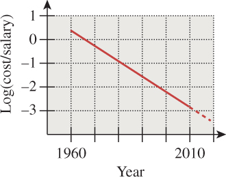
Figure 1.6: The log of the ratio between the cost of a computer and the salary of a person using the computer (roughly amortized for multiuser systems), plotted against the year.
What sorts of issues affect UI design? Many of them are related to psychology, perception, and the general area called human factors. It’s one thing to use color in your UI; it’s another to make sure the UI works for color-deficient users as well. It’s one thing to have all necessary menu items present; it’s another to order and group them so that a typical user can find what s/he is looking for quickly and select it easily: The menu items must be organized, and each item must be large enough to make the selection process easy. And it’s still another thing to be certain that your UI is appropriate for whatever kind of device you might be using: a desktop machine, a smartphone, a PDA, or a video game controller.
Despite the importance of interfaces, we will not discuss them much; UI research is now its own field, related to graphics but no longer a part of it. In some cases, there are interface elements for which those with experience in graphics can offer particular insight. Chapter 21 discusses some of these as applications of the modeling and transformation technology developed earlier in the book.
From this discussion, it’s clear that the goals of computer graphics are not purely based on physics or algorithms, but they depend critically on human beings. We don’t merely compute the transfer of light energy in a scene; we must also consider the human perception of the results: Was the extra computation time used in a way that mattered to the viewer? We don’t merely create an application program that provides functionality and performance that are appropriate for the some particular endeavor (e.g., playing music from a library or helping a physician maintain notes on patients); we also concern ourselves with whether the interface the program presents makes the program easy to use. Ease of use is obviously closely tied to human perception. We therefore present an introduction to perception in Chapter 5.
1.2. A Brief History
Graphics research has followed a goal-directed path, but one in which the goal has continued to shift; the first researchers worked in a context of limited processor power, and thus they frequently made choices that got results as quickly and easily as possible. Early efforts were divided between trying to make drawings (e.g., blueprints) and trying to make pictures (e.g., photorealistic images). In each case, many assumptions were made, usually in concession to available processor power and display technologies. When a single display cost as much or more than an engineer’s salary, every picture displayed had to have some value. When displaying a few hundred polygons took minutes, approximating curved surfaces with relatively few polygons made a lot of sense. And when processor speeds were measured in MIPS (millions of instructions per second) but images contained 250,000 or 500,000 pixels, one could not afford to perform a lot of computations per pixel. (In the 1960s and early 1970s, many institutions had at most a single graphical display!) Typical simplifying assumptions were that all objects reflected light more or less as flat latex paint does (although some more-sophisticated reflectance models were used in a few systems), that light either illuminated a surface directly or bounced around in the scene so often that it eventually provided a general ambient light that illuminated things even when they weren’t directly lit, and that the colors at the interior points of any triangle could be inferred from the colors computed at the triangle’s vertices.
Gradually, richer and richer models—of shape, of light, and of reflectance—were added, but even today the dominant model for describing the light in a scene includes the term “ambient,” meaning a certain amount of light that’s “all over the place in the scene” without any clear origin, ensuring that any object that’s visible in the scene is at least somewhat illuminated. This ad hoc term was added to address aspects of light transport, such as interobject reflections, that could not be directly computed with 1960s computers; but it remains in use today. While many books follow the historical development of light transport, we’ll choose a different approach and discuss the ideal (the physical simulation of light transport), how current algorithms approximate that ideal, how some earlier approaches did so as well, and how the vestiges of those approximations remain in common practice. The exception to this is that we’ll introduce, in Chapter 6, a reflectance model that represents the scattering of light from a surface as a sum of three terms: “diffuse,” corresponding to light that’s reflected equally in all directions; “specular,”4 used to model more directional reflection, ranging from things like rough plastic all the way to the nearly perfect reflection of mirrors; and ambient. We will refine this model somewhat in Chapter 14, and then examine it in detail in Chapter 27. The advantage of the early look is that it allows you to experiment with modeling and rendering scenes early, even before you’ve learned how light is actually reflected.
4. The word “specular” has multiple meanings in graphics, from “mirrorlike” to “anywhere from sort of glossy to a perfect mirror.” Aside from its use in Chapter 6 we’ll use “specular” as a synonym for mirror reflection, and “glossy” for things that are shiny but not exactly mirrorlike.
Graphics displays have improved enormously over the years, with a shift from vector devices to raster devices—ones that display an array of small dots, for example, like CRTs or LCD displays—in the 1970s to 1980s, and with steadily but slowly increasing resolution (the smallness of the individual dots), size (the physical dimensions of the displays), and dynamic range (the ratio of the brightest to the dimmest possible pixel values) over the past 25 years. The performance of graphics processors has also progressed in accordance with Moore’s Law (the rate of exponential improvement has been greater for graphics processors than for CPUs). Graphics processor architecture is also increasingly parallel; how far this can go is a matter of some speculation.
In both processors and displays, there have also been important leaps along with steady progress: The switch from vector devices to raster displays, and their rapid infiltration of the minicomputer and workstation market, was one of these. Another was the introduction of commodity graphics cards (and their associated software), which made it possible to write programs that ran on a wide variety of machines. At about the same time as raster displays became widely adopted another major change took place: the adoption of Xerox PARC’s WIMP GUIs. This is when graphics moved from being a laboratory research instrument to being an unspoken component of everyday interaction with the computer.
One last leap is worth noting: the introduction of the programmable graphics card. Instead of sending polygons or images to a graphics card, an application could now send certain small programs describing how subsequent polygons and images were to be processed on their way to the display. These so-called “shaders” opened up whole new realms of effects that could be generated without any additional CPU cycles (although the GPU—the Graphics Processing Unit—was working very hard!). We can anticipate further large leaps in graphics power in the next few decades.
1.3. An Illuminating Example
Let’s now look at a simple scene and ask ourselves how we can make a picture of it.
A 100 W pinpoint lamp hangs above a table that’s painted with gray latex paint at a height of 1 m, in an otherwise dark room. We look at the table from above, from 2 m away. What do we see? Regardless of the visible-light output of the lamp and the exact reflectivity of the surface, the pattern of illumination in the scene—brighter just beneath the lamp, dimmer as we move away—is determined by physics. We can do a thought experiment and imagine an ideal “picture” of this scene. And we can hope that a computer graphics system, asked to render a picture of this scene, would produce a result that would be a good approximation of this picture.
Nonetheless, it’s difficult to write a conventional program with a standard graphics package to even display the general pattern of illumination. Most standard packages have no notion of units like “meters” or “grams” or “joules”; even their descriptions of light omit any mention of wavelength. Furthermore, conventional graphics packages compute the brightness of incoming light in a way that varies with the distance from the source. However, it does not vary as 1/d2, as we know it must from physics, but rather according to a different rule. To be fair, one can make the conventional package have a quadratic falloff, but the resultant picture still looks wrong.5 That’s in part because of nonlinearities in displays and the use of a small range of values (typically 0 to 255) to represent light amounts, together with the limited dynamic range of many displays (one cannot display very brightly lit or very dimly lit things faithfully). Using a linear falloff (often with a small quadratic term mixed in) partly compensates for these and results in a better-looking picture. But it’s really just an ad hoc solution to a collection of other problems.
5. The wrongness is not from the unfamiliarity of the point-light source; even if we made a graphical model of a larger-area light source, the results would be wrong.
To correctly make a picture of the simple scene described above, it’s probably best to model the physics directly and only then worry about the display of the resultant data. By the end of Chapter 32 you’ll be able to do so.
In asking for a physically correct result in this example, we’re examining a particular area of graphics—that of realism. It’s remarkable that the quest for realism should have gone so very well in the early years of graphics, given the lack of any physical basis for most of the computations. This can be attributed to the remarkable robustness of the human visual system (HVS): When we present to the eyes anything that remotely resembles a physically realistic image, our visual system somehow makes sense of it. More recent trends in which captured imagery (e.g., digital photographs) are combined with graphics imagery have shown how important it can be to get things right: A mismatch in the brightness of real and synthetic objects is instantly noticeable.
But often in graphics we seek not a physical simulation but a way to present information visually (like a book or newspaper layout). In these cases, the typical viewing situation is a well-lit room, with light of approximately constant intensity arriving from all directions, and with the reflectance of the items on the page varying by a factor of perhaps 103. Simply setting the intensities of screen pixels to reasonable values that vary over a similar range works well, and there’s no reason to do a physical simulation of the reflecting page. However, there may be a reason to be sure that what’s displayed is faithful to the original (i.e., that the colors you see on your display are the same ones I see on mine); displays of fashion items or paint colors need to be accurate for users to understand how they really look.
Indeed, such a situation is a good opportunity for abstraction, which is a key element in visual communication in general: Because the physical characteristics of the document will not have a large impact on the viewer’s experience as s/he encounters it, one can instead discuss the document in more abstract terms of shape and color and form. It’s imperative, of course, that these abstractions capture what’s important and leave out what’s unimportant about whatever is being discussed; this is a key characteristic of the process of modeling, which we will return to frequently throughout this book.
1.4. Goals, Resources, and Appropriate Abstractions
The lightbulb example gives us another principle: In any simulation, first understand the underlying physical or mathematical processes (to the degree they’re known), and then determine which approximations will best provide the results we need (our goals), given the constraints of time, processor power, and similar factors (our resources).
This approach applies both to 2D display graphics—the kinds of graphical objects found in the interface to your web browser, for instance, like the buttons that help you navigate and the display of the successive lines of text—and to 3D renderings used for special effects. In the former case, the dominant phenomena may not be those of physics but of perception and design, but they must still be understood. In addition to choosing a rich-enough abstraction, part of modeling wisely is choosing the right representation in which to work: To represent a real-valued function on a plane, you might use a rectangular array of values; divide the plane into triangular regions of various shapes and sizes, with values stored at the triangle vertices (this is common when making models of things like fluid flow); or use a data structure that stores the rectangular value array in such a way that whenever adjacent values agree they are merged into a larger “cell” so that detail is only present in the areas where the function is changing rapidly.
We summarize the preceding discussion in a principle:
![]() The Wise Modeling Principle
The Wise Modeling Principle
When modeling a phenomenon, understand the phenomenon you’re modeling and your goal in modeling it, then choose a rich-enough abstraction, and then choose adequate representations to capture your abstraction within the bounds of your resources. Once this is done, test to verify that your abstraction was appropriate.
The testing will vary with the situation: If the design abstracts something about human perception, then the test may involve user studies; if the design abstracts something physical (“We can safely model small ocean waves with sinusoids”), then the test may be quantitative.
Barzel [Bar92] argues that most physical models for computer graphics come in three parts: the physical model itself, a mathematical model, and a numerical model. (As an example, the physical model might be that ocean waves are represented by vertical displacements of the water’s surface, and their motion is governed solely by the forces arising from differences in nearby heights [rather than by wind, for example]; the mathematical model might be that these displacements are represented by time-dependent functions defined at integer points in some coordinate grid on the ocean’s surface, with intermediate values being interpolated; and the computational model might be that the water’s state one moment in the future can be determined from its state now by approximating all derivatives with “finite differences” and then solving a linearized version of the resultant equations.) Including this separation in your programs can help you debug them. This means, however, that during debugging, you must remember your model and its level of abstraction and the limitations these impose on your intended results. (In our example, the physical model itself says that you cannot hope to see breaking waves, while the mathematical model says that you cannot hope to see details of the water’s surface at a scale smaller than the coordinate grid.) Within computer science, this is very unusual: In most other areas of computer science, you’ve got either a computational model or a machine model, and this single model provides your foundation. In graphics, we have physical, mathematical, numerical, computational, and perceptual models, all interacting with one another.
In both 2D and 3D graphics, it’s critically important to consider the eventual goal of your work, which is usually communication in some form, and usually communication to a human. This end goal influences many things that we do, and should influence everything. (This is just a restatement of the “form follows function” dictum, as valuable in graphics as it is anywhere else.) As a simple example, consider how we treat light, which is just a kind of electromagnetic radiation: Because humans can only detect certain frequencies of light with their eyes, we usually don’t worry about simulating radio waves or X-rays in graphics, even though the light emitted by conventional lamps (and the sun) includes many energies outside the visible spectrum. Hence, a limitation of the visual system becomes a computational savings for our programs. Similarly, because the eye’s sensitivity to light energy is approximately logarithmic, we build our display hardware (to a first approximation) so that equal differences in pixel values correspond to equal ratios of displayed light energy.
![]() The Visual System Impact Principle
The Visual System Impact Principle
Consider the impact of the human visual system on your problem and its models.
As another example, even in 2D display graphics there are perceptual issues to consider: The limits of human visual acuity tell us that the things we display must be of a certain size to be perceptually meaningful; at the same time, the limits of human motor control tell us that interaction must be designed in ways that fit those limits. We cannot ask a user to click on a sequence of pixels in a 1280 × 1024-pixel, 17-inch display with an ordinary mouse—clicking on a particular pixel is virtually impossible.
We don’t mean to suggest that perception should influence every decision made in graphics; in Chapter 28 we’ll see the risks that arise from treating light throughout the rendering process in a way that captures only our three-dimensional perception of color rather than the full spectral representation. However, in many situations where the range of brightness is small, the logarithmic nature of the eye’s sensitivity is not particularly important, and common practice therefore often involves such things as averaging pixel values that represent log brightnesses; such techniques often serve their purposes admirably.
1.4.1. Deep Understanding versus Common Practice
Because computer graphics is actually in use all around us, we have to make concessions to common practice, which has generally evolved because it produced good-enough results at the time it was developed. But after a discussion of common practice, we’ll often have a stand-back-and-look critique of it as well so that the reader can begin to understand the limitations of various approaches to graphics problems.
1.5. Some Numbers and Orders of Magnitude in Graphics
Because we will start our study of graphics with a discussion of light, it’s useful to have a few rough figures characterizing the light encountered in ordinary scenes. Visible light, for instance, has a wavelength between approximately 400 and 700 nanometers (a nanometer is 1.0 × 10⁻⁹ m). A human hair has a diameter of about 1.0 × 10⁻⁴ m, so it’s about 100 to 200 wavelengths thick, which helps give a human scale to the phenomena we’re discussing.
1.5.1. Light Energy and Photon Arrival Rates
A single photon (the indivisible unit of light) has an energy E that varies with the wavelength λ according to
where h ≈ 6.6 × 10⁻³⁴ J sec is Planck’s constant and c ≈ 3 × 10⁸ m/sec is the speed of light; multiplying, we get
Using 650 nm as a typical photon wavelength, we get
as the energy of a typical photon.
An ordinary 100 Watt incandescent bulb consumes 100 W, or 100 J/sec, but only a small fraction of that—perhaps 2% to 4% for the least efficient bulbs—is converted to visible light. Dividing 2 J/sec by 3 × 10–19 J, we see that such a bulb emits about 6.6 × 10¹⁸ visible photons per second. An office—say, 4 m × 4m × 2.5 m—together with some furniture has a surface area of very roughly 100 m2 = 1 × 106 cm2; thus, in such an office illuminated by a single 100 W bulb on the order of 1012 photons we arrive at a typical square centimeter of surface each second.
By contrast, direct sunlight provides roughly 1000 times this arrival rate; a bedroom illuminated by a small night-light has perhaps 1/100 the arrival rate. Thus, the range of energies that reach the eye varies over many orders of magnitude. There is some evidence that the dark-adapted eye can detect a single photon (or perhaps a few photons). At any rate, the ratio between the daytime and nighttime energies of the light reaching the eye may approach 1010.
1.5.2. Display Characteristics and Resolution of the Eye
Because we also work with computer displays, and the computers driving these displays typically draw polygons on the screen, it’s valuable to have some numbers describing these. A typical 2010 display had between 1 million and 1.5 million pixels (individually controllable parts of the display6)—which will soon grow to 4 million pixels; with displays that are 37 cm (about 15 inches) wide, the diagonal distance between pixel centers is on the order of 0.25 mm. The dynamic range of a typical monitor is about 500:1 (i.e., the brightest pixels emit 500 times the energy emitted by the darkest pixels). The display on a well-equipped 2010 desktop subtended an angle of about 25° at the viewer’s eye.
6. Each display part may actually consist of several pieces, as in a typical LCD display in which the red, green, and blue parts are three parallel vertical strips that make up a rectangle, or may be the result of a combination of multiple things, like the light emitted by the red, green, and blue phosphors of each triad of phosphors on a CRT screen.
The human eye has an angular resolution of about one minute of arc; this corresponds to about 300 mm at a 1 km distance, or (more practical for viewing computer screens) about 0.3 mm at a 1 m distance. When pixels get about half as large as they are now, it will be nearly impossible for the eye to distinguish them.7 A one-pixel shift in a single character’s position on a line of text may be completely unnoticeable. Furthermore, the eye’s resolution far from the center of the view is much less, so pixel density at the edge of the display screen may well be wasted much of the time. On the other hand, the eye is very sensitive to motion, so two adjacent pixels in a gray region that alternately flash white may give an illusion of motion that’s easily detectable, which might be useful for attracting the user’s attention.
7. This doesn’t mean it won’t be worth further reducing their size; 300 dot-per-inch (dpi) printers use dots that are about 0.1 mm, and their quality is noticeably poorer than that of 1200 dpi printers, even when viewed at a distance of a half-meter. Distinguishing between adjacent pixels and detecting the smoothness of an overall image are evidently rather different tasks.
1.5.3. Digital Camera Characteristics
The lens of a modern consumer-grade digital camera has an area of about 0.1 cm2; suppose that we use it to photograph a typical 100 W incandescent bulb, filling the frame with the image of the bulb. To do so, we place the lens 10 cm from the bulb. The surface area of a sphere with radius 10 cm is about 1200 cm2; our lens therefore receives about 1/10,000 of the light emitted by the bulb, or 6.6 × 10¹⁴ photons per second. If we take the picture with a 0.01 sec exposure and we have an approximately 1-million-pixel sensor, then each sensor pixel receives about 106 photons. Photographing a dark piece of carpet in our imaginary office above might result in each sensor pixel receiving only 100 photons.
1.5.4. Processing Demands of Complex Applications
Computer games are some of the most demanding applications at present; to make objects appear on the user’s screen, these applications send polygons to a graphics processor. These polygons have various attributes (like color, texture, and transparency) and are displayed with various technologies (antialiasing, smooth shading, and others, all of which we’ll discuss in detail later). For a polygon to be displayed, certain pixels must be colored in certain ways. Thus, polygon rate (the number of polygons displayed per second) and fill rate (the number of pixels colored per second) are both used to measure performance. The numbers are constantly changing, and there’s a huge difference between a textured, antialiased, transparent polygon covering 500 pixels and a flat-shaded 10-pixel triangle, so comparisons are difficult. But complex scenes for interactive display can easily contain 1 million polygons, of which maybe 100,000 are visible (the others being hidden by things in front of them or outside the field of view), each occupying perhaps 10 pixels on average. In many cases, a single polygon occupies less than a single pixel. This happens in part because complex shapes are often modeled with polygonal meshes (see Figure 1.7). For high-quality, noninteractive, special-effects production, the resolution of the final image may be considerably higher, but at the same time, scenes can contain many millions of polygons; the “polygon is smaller than a pixel” rule of thumb continues to apply.
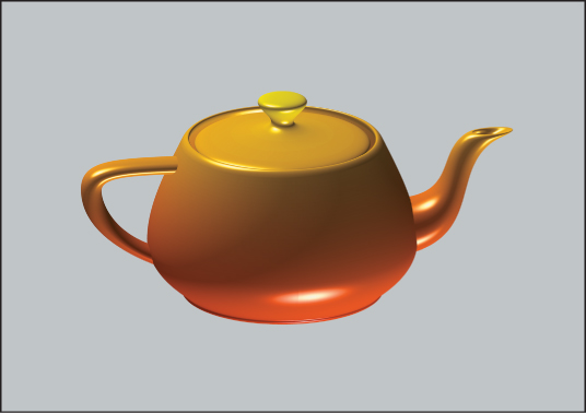
Figure 1.7: The standard teapot, created by Martin Newell, a model that’s been used thousands of times in graphics.
1.6. The Graphics Pipeline
The functioning of a standard graphics system is typically described by an abstraction called the graphics pipeline. The term “pipeline” is used because the transformation from mathematical model to pixels on the screen involves multiple steps, and in a typical architecture, these are performed in sequence; the results of one stage are pushed on to the next stage so that the first stage can begin processing the next polygon immediately.
Figure 1.8 shows a simplified view of this pipeline: Data about the scene being displayed enters at various points to produce output pixels.
For many purposes, the exact details of the pipeline do not matter; one can regard the pipeline as a black box that transforms a geometric model of a scene and produces a pixel-based perspective drawing of those polygons. (Parallel-projection drawings are also possible, but we’ll ignore these for the moment.) On the other hand, some understanding of the nature of the processing is valuable, especially in cases where efficiency is important. The details of the boxes in the pipeline will be revealed throughout the book.
Even with this simple black box you can write a great many useful programs, ignoring all physical considerations and treating the transformation from model to image as being defined by the black box rather than by physics (like the non-quadratic light-intensity falloff mentioned above).
The past decade has, to some degree, made the pipeline shown above obsolete. While graphics application programming interfaces (APIs) of the past provided useful ways to adjust the parameters of each stage of the pipeline, this fixed-function pipeline model is rapidly being superseded in many contexts. Instead, the stages of the pipeline, and in some cases the entire pipeline, are being replaced by programs called shaders. It’s easy to write a small shader that mimics what the fixed-function pipeline used to do, but modern shaders have grown increasingly complex, and they do many things that were impossible to do on the graphics card previously. Nonetheless, the fixed-function pipeline makes a good conceptual framework onto which to add variations, which is how many shaders are in fact created.
1.6.1. Texture Mapping and Approximation
One standard component of the black box is the texture map. With texture mapping, we take a polygon (or a collection of polygons) and assign a color to each point via a lookup in a texture image; the technique is a little like applying a stencil to a surface or gluing a decal onto an object. You can think of the texture image, which can be a piece of artwork scanned into the system, a photo taken with a digital camera, or an image created in a paint program, for instance, as a rubber sheet with a picture on it. The texture coordinates describe how this sheet is stretched and deformed to cover some part of the object.
The idea of using a texture to modify the color characteristics of each point of an image is only one of many applications of texture mapping. The central ideas of texture mapping have been generalized and applied to many surface properties. The appearance of a surface, for instance, depends in part on the surface’s normal vector (or normal), which is the vector that’s perpendicular to the surface at each point. This normal vector is used to compute how light reflects from the surface. Since the surface is typically represented by a mesh of polygons, these surface normal vectors are usually computed at the polygon vertices and then interpolated over the interior of the polygon to give a smooth (rather than faceted) appearance to the shape.
If instead of using the true normal to a surface (or its approximation by interpolation as above) we use a substantially different one at different points of each polygon, the surface will have a different appearance at different points, appearing to tilt more toward or away from us, for instance. If we apply this idea across a whole surface we can generate what seems to be a lumpy surface (see Figure 1.9), while the underlying shape is actually nearly smooth.
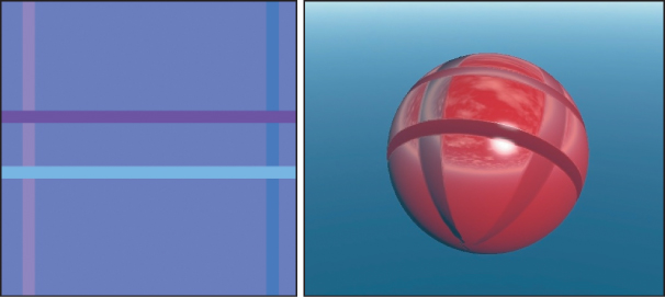
Figure 1.9: (a) The image at left depicts a normal map. Each image point has x- and y-coordinates that correspond to the latitude and longitude of a point on the sphere. The RGB color triple stored at each point determines how much to tilt the normal vector at the corresponding point of the sphere. The pale purple color indicates no tilt, while the four stripes tilt the normal vector up and down or left and right. (b) The resultant shape, which looks bumpy; you can tell it’s actually smooth by looking at the silhouette. Note that it has also been “color textured” with a reflected sky.
The surface appears to have lots of geometric variation even though it’s actually spherical. Unfortunately, near the silhouette of the surface the unvarying nature is evident; this is a common limitation of such mapping tricks. On the other hand, being able to draw just a few normal-mapped polygons instead of thousands of individual ones can be enough of an advantage to make this choice appropriate. This kind of choice is commonplace in graphics—one must decide between physical correctness (which might require huge models) and approximately correct imagery made with smaller models. If model size and processing time constitute a significant portion of your engineering budget, these are the sorts of tradeoffs you have to make.
1.6.2. The More Detailed Graphics Pipeline
As we said above, a pipeline architecture lets us process many things simultaneously: Each stage of the pipeline performs some task on a piece of data and hands the result to the next stage; the original pipeline stage can then begin performing the task on the next piece of data. When such a pipeline is properly designed this can result in improved throughput, although as stages are added, the total amount of time it takes for an input datum to produce a result continues to increase. In systems where interactive performance is critical, this lag or latency can be important.
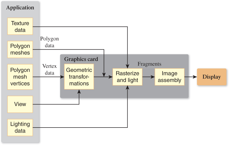
The graphics pipeline consists of four main parts: vertex geometry processing and transformation, triangle processing (through rasterization) and fragment generation, texturing and lighting, and fragment-combination operations for assembling the final image, all of which we’ll summarize presently (and which are covered in more detail in Chapters 15 and 38). You can think of this pipeline as part of a larger pipeline that captures the structure of a typical program (see Figure 1.10, in which the vertex processing portion is labeled “Geometric transformation”; the fragment generation, texturing, and lighting are collected into a single box; and the portion representing the final processing of fragments is labeled “Image assembly”).
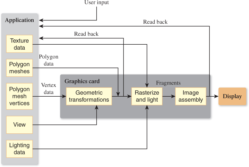
Figure 1.10: In this depiction of a larger graphics pipeline, the application program performs some work (e.g., animation) to determine the geometry to be displayed; this geometric description is handed to the graphics pipelines; the resultant image is displayed. At the same time, user input, in response to the displayed image, may affect the next operations of the application program, as may data read back from the graphics pipeline itself.
In this larger pipeline, an application program generates data to be displayed, and the graphics pipeline displays it. But there may be user input (possibly in response to the displayed images) that controls the application, as well as information read back from the graphics pipeline and also used in the computation of the next image to be shown.
Each part of the graphics pipeline may involve several tasks, all performed sequentially. The exact implementations of these tasks may vary, but the user of such a system can still regard them as sequential; graphics programmers should have this abstraction in mind while creating an application. This programmer’s model is the one provided by most APIs that are used to control the graphics pipeline. In actual practice (see Chapter 38), the exact order of the tasks within the parts (or even the parts to which they are allocated) may be altered, but a graphics system is required to produce results as if they were processed in the order described. Thus, the pipeline is an abstraction—a way to think about the work being done; regardless of the underlying implementation, the pipeline allows us to know what the results will be.
The vertex geometry part of the pipeline is responsible for taking a geometric description of an object, typically expressed in terms of the locations of certain vertices of a polygonal mesh (which you can think of informally as an arrangement of polygons sharing vertices and edges to cover an object, i.e., to approximate its surface), together with certain transformations to be applied to these vertices, and computing the actual positions of the vertices after they’ve been transformed. The polygons of the mesh, which are defined in terms of the vertices, are thus implicitly transformed as well.
The triangle-processing stage takes the polygons of the mesh—most often triangles—and a specification for a virtual camera whose view we are rendering, and processes the polygons one by one in a process called rasterization, to convert them from a continuous-geometry representation (triangle) into the discrete geometry of the pixelized display (the collection of pixels [or portions of pixels] that this triangle contains).
The resultant fragments (pixels or portions of pixels that belong to the triangle and may eventually appear on the display if they’re not obscured by some other fragment) are then assigned colors based on the lighting in the scene, the textures (e.g., a leopard’s spots) that have been assigned to the mesh, etc.
If several fragments are associated to the same pixel location, the frontmost fragment (the one closest to the viewer) is generally chosen to be drawn, although other operations can be performed on a per-pixel basis (e.g., transparency computations, or “masking” so that only certain fragments get “drawn,” while others that are masked are left unchanged).8
8. Note that the choice of a representation by a raster grid implies something about the final results: The information in the result is limited! You cannot “zoom in” to see more detail in a single pixel. But sometimes in computing, what should be displayed in a single pixel requires working with subpixel accuracy to get a satisfactory result. We’ll frequently encounter this tension between the “natural” resolution at which to work (the pixel) and the need to sometimes do subpixel computations.
In modern systems, all of this work is usually done on one or more Graphics Processing Units (GPUs), often residing on a separate graphics card that’s plugged into the computer’s communication bus. These GPUs have a somewhat idiosyncratic architecture, specially designed to support rapid and deep pipelining of the graphics pipeline; they have also become so powerful that some programmers have started treating them as coprocessors and using them to perform computations unrelated to graphics. This idea—having a separate graphics unit that eventually becomes so powerful that it gets used as a (nongraphics) coprocessor—is an old one and has been reinvented multiple times since the 1960s. In early generations, this coprocessor was typically moved closer and closer to the CPU (e.g., sharing memory with the CPU) and grew increasingly powerful until it became so much a part of the CPU that designers began creating a new graphics processor that was closely associated to the display; this was called the wheel of reincarnation in a historically important paper by Myer and Sutherland [MS68]. The notion may be slightly misleading, however, as observed by Whitted [Whi10]: “We sometimes forget that the famous ‘wheel of reincarnation’ translates as it rotates, transporting us to unfamiliar technological territory even if we recognize historical similarities.”
1.7. Relationship of Graphics to Art, Design, and Perception
The simple lamp at the top of Figure 1.11 conveys both a shape and a design style in just a few strokes. Henri Matisse’s “Face of a Woman,” shown at the bottom of Figure 1.11, contains no more than 13 pen strokes but is nonetheless able to convey an enormous amount to a human viewer; it’s far more recognizable as a face than many of the best contemporary face renderings in graphics. This is partly because of the uncanny valley—an idea from robotics [Mor70] that states that as robots got increasingly humanlike, a viewer’s sense of familiarity would increase to a point, but then it would drop precipitously until the robot was very human-like, at which point the familiarity would rise rapidly above its previous level. The uncanny valley is the region in which familiarity is low but human resemblance is high. In the same way, graphics images of humans that are “almost right” are often described as “creepy” or “weird.” But ignoring this for a moment, there’s another important difference: Matisse’s drawing is simple, whereas an enormous amount of computational effort is expended in making a realistic face rendering. This is because artists and designers have reverse-engineered the human visual system to get the greatest effect for the least amount of “drawing budget.” Looking at their work helps us understand that the goal of all graphics is communication, and that sometimes this is best achieved not with realism but with other means. Auto-repair manuals, for instance, can be illustrated with photos, but the top-quality manuals are instead illustrated with drawings (see Figure 1.12) that emphasize important details and elide other details. Which details are important? That depends on the intent of the person creating the image and on the human visual system. We know, for instance, that the human visual system is sensitive to sharp transitions in brightness and is somewhat more sensitive to vertical and horizontal lines than to diagonal ones; this partly explains why line drawings are effective, and why one can afford to leave out diagonal lines preferentially over verticals and horizontals.
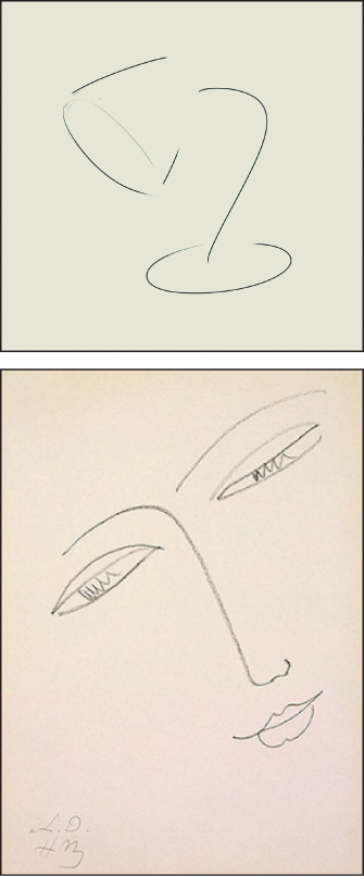
Figure 1.11: The lamp, courtesy of Jack Hughes, has just five strokes. Matisse’s “Face of a Woman” depicts both shape and mood in just 13 strokes.

In every engineering problem, there’s a budget; graphics is no different. You are limited in graphics by things like the number of polygons you can send to the pipeline before you have to draw the next frame to display, the number of pixels that can be filled, and the amount of computation you can afford to do in the CPU to decide what polygons you want to draw in the first place. Artists who are drawing something have a similar budget: the amount of effort spent in placing marks on a page, the time before the scene being rendered changes (you can’t paint a sunset-in-progress at midnight), etc. They’ve developed techniques that allow them to convey a scene on a low budget: For instance, contour drawings work well, and flat fill-in color adds contrast that helps separate individual objects, etc. We can learn from the artists’ reverse engineering of the human visual system and use their techniques to render more efficiently. And because most computer-generated images are intended to be viewed by a human, the human brain is the ultimate measurement tool for what’s satisfactory. There’s another budget to consider as well: the viewer’s attention. Graphics is also limited by the time and effort the human viewer can be expected to spend to understand what is being communicated. Of course, our standard for satisfaction varies with time: The images produced in the 1960s and 1970s seemed amazing at the time, but are completely unsatisfactory by today’s standards.
On the other hand, sometimes the nature of the visual system lets us make very effective but simple approximations of reality that are entirely convincing; early cloud models [Gar85] used extremely simple approximations of cloud shapes very effectively, because the eye is not terribly sensitive to the geometry of a cumulus cloud, as long as it looks fluffy. But all too often, such simplifications fail badly. For instance, we could attempt to make a mesh appear to have a smoothly changing color by filling each triangle with its own color (flat shading) and then making the individual triangles small so that the changes from one triangle to the next are tiny. Unfortunately, unless the triangles are very tiny, this leads to something called Mach banding (see Figure 1.13), which is extremely distracting to the eye.

Figure 1.13: Each strip is a single color, but the left side of each strip looks a little brighter and the right side looks a little darker, which has the effect of accentuating the dividing line between the strips; this effect is known as Mach banding.
1.8. Basic Graphics Systems
A modern graphics system consists of a few interaction devices (keyboard, mouse, perhaps a tablet or touch screen), a CPU, a GPU, and a display. Today’s displays are either liquid-crystal displays (LCDs) or cathode-ray tube (CRT) displays, although new technologies like plasma displays and OLEDs (organic light-emitting diodes) are constantly changing the landscape. Each displays a rectangular array of pixels, or regions that can be lit to varying degrees in varying colors by the control of three colored parts, typically red, green, and blue. In the case of a CRT, when a single pixel is turned on it produces a glowing, approximately circular area containing an RGB triad of phosphors on the screen, an area that is bright in the center and rapidly fades at the edges so that the bright areas of adjacent pixels overlap only a little. In the case of an LCD, there is a backlight behind the screen, and each pixel is a set of three small rectangles that allow some amount of the backlight in the red, green, or blue spectrum to pass through to the viewer. There is a very small space between the pixels (like the grout on a tile floor), but for most purposes we can treat the LCD pixels as completely covering the screen. The brightness of each pixel (on either type of display) can be controlled by a program; we can also assume, except in the most rigorous situations, that all pixels are capable of displaying the same brightnesses, and that there is no substantial variation of their apparent brightness with position (i.e., pixels at the display’s edge look just as bright as those at the center when they’re “turned on” to the same degree).
A typical graphics program runs on the CPU, processing input from the UI devices and sending instructions to the GPU describing what should be displayed; this, in turn, prompts further user interaction, and the cycle continues. In almost all cases, this structure is provided by a graphics platform that serves as an intermediary between a graphics application and the hardware, but for now, let’s consider the simple case where we’re building a basic graphics program from scratch. Frequently the display is steadily changing (e.g., it is being updated every 1/30 of a second), and user input may come only occasionally. The simplest model for the application program is to issue for each redisplay cycle new display instructions to the GPU, often resulting in a frame rate that’s typically 15 to 75 frames per second. Too-low frame rates can severely degrade the quality of interaction, as can too-great latency (the time between an action—be it a user-initiated click, or the initiation of a frame redisplay—and its effect), so this simple model must be used with caution.
1.8.1. Graphics Data
Typically graphical models are created in some convenient coordinate system; a cube that is to be used as one of a pair of dice might be modeled as a unit cube, centered at the origin in 3-space, with all x-, y-, and z-coordinates between –0.5 and 0.5. This coordinate system is called modeling space or object space.
This cube is then placed in a scene—a model of a collection of objects and light sources. Perhaps the dice are on a table that’s six units tall in y; in the scene description, they’re moved there by applying some transformation to the coordinates of all the vertices (the corners) of the cube. In the case of the die, perhaps all six vertices have 6.5 added to their y-coordinates so that the bottom of the die sits on the top of the table. The resultant coordinates are said to be in world space (see Figure 1.14). (Chapter 2 describes an example of this modeling process in great detail.)
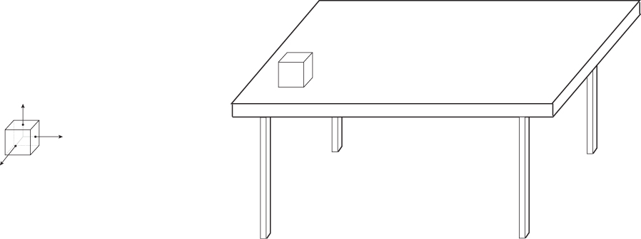
Figure 1.14: On the left, a die is centered on its own axes in modeling coordinates. The same die is placed in the world (on the right) by adding 6.5 to each y-coordinate (the y-direction points “up”) to get world coordinates for the die.
The location and direction of a virtual camera is also given in world space, as are the positions and physical characteristics of virtual lights. Consider a set of coordinate axes (see Figure 1.15) whose origin is at the center of the virtual camera, whose x-axis goes to the right side of the camera (as seen from the back), whose y-axis points up along the back of the camera, and whose negative z-axis points along the camera view. All objects in world space have coordinates in this coordinate system as well; these coordinates are called camera-space coordinates or simply camera coordinates. Computing these camera-space coordinates from world coordinates is relatively simple (Chapter 13) and is one of the services typically provided by a graphics platform.
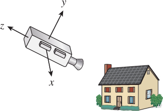
Figure 1.15: The virtual camera looks at a scene from a specified location, and with some orientation or attitude. We can create a coordinate system whose origin is at the center of the camera, whose z-axis points opposite the view direction, and whose x- and y-axes point to the right and to the top of the camera, respectively. The coordinates of points in this coordinate system are called camera coordinates.
These camera coordinates are transformed into normalized device coordinates, in which the visible objects have floating-point xy-values between –1 and 1, and whose z-coordinate is nonpositive. (Objects with xy-values outside this range are outside the camera’s field of view; objects with z > 0 are behind the camera rather than in front of it.) Finally, the visible fragments are transformed to pixel coordinates, which are integers (with (0, 0) being the upper-left corner of the display and (1280, 1024) being the lower-right corner of the display) by scaling and rounding the xy-coordinates. These resultant numbers are sometimes said to be coordinates in image space. Returning to the cube that’s to be used as one of a pair of dice, we want each side of the cube to look like the side of a die. To do this, we might use a texture map containing a picture of each side of a die. The vertices9 of each face of the cube will then also be given texture coordinates indicating what portion of the texture should be applied to them (see Figure 1.16).
9. The word “vertices” (VERT-uh-sees) is the plural of “vertex,” although “vertexes” is sometimes used. Occasionally our students mistakenly back-construct the singular “vertice.” Please avoid this. Other similarly formed plurals are index–indices and simplex–simplices.
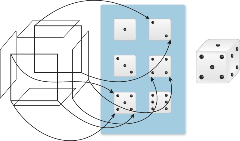
Figure 1.16: The vertices of each of the six faces of the die (shown in an exploded view) are assigned texture coordinates (a few are indicated by the arrows in the diagram); the texture image is then used to determine the appearance of each face of the die, as if the texture were a rubber sheet stretched onto the face. Note that a single 3D location may have many texture coordinates associated to it, because it is part of many different faces. In the case of the die, this is moot, because all instances of the 3D point get the same texture color assigned. Chapter 20 discusses topics like this at greater length. The resultant textured die is shown on the right.
The various conversions from the continuous geometry of Euclidean space to the rasterized geometry of the screen (with rasterized textures being used along the way) involve many subtleties, to be discussed in Chapter 18.
1.9. Polygon Drawing As a Black Box
Given the difficulties of carrying out the steps in the pipeline (especially those that involve the transformation from continuous to discrete geometry), we can, for the time being, treat polygon drawing as a black box: We have a graphics system which, when told to draw a polygon, somehow makes the right pixels on the display be illuminated with the right colors. This black-box approach will let us experiment with interaction, color, and coordinate systems. We’ll then return to the details in later chapters.
1.10. Interaction in Graphics Systems
Graphics programs that display images in some form typically feature some level of user interaction as well. For example, in many programs the user clicks on things with the mouse, selects menu items, and types at the keyboard. However, the level of interaction in some programs (indeed, in many 3D games) is far more complex.
Graphics programs typically support such interaction by having two parallel threads of execution; one thread handles the main program and the other handles the GUI. Each component of the GUI—button, checkbox, slider, etc.—is associated with a callback procedure in the main program. For instance, when the user clicks a button the GUI thread calls the button’s callback procedure. That procedure in turn may alter some data, and may also ask the GUI to change something.
As an example, imagine a trivial game in which a user has to guess a number that the computer has chosen—either one, two, or three. To do so, the user clicks on one of three buttons. If the user clicks on the correct button, the display reads “You win!”; if not, it reads “Try again.” In this scenario, when the user clicks button 2 but the secret number is 1, the button-2 callback does the following.
1. It checks to see whether 2 was the secret number.
2. Because 2 is not the secret number, it asks the GUI to display the “try again” message.
3. It asks the GUI to gray out (disable) the “2” button so that the user is not able to guess the same wrong answer more than once.
Of course, the button-1 and button-3 callbacks would be very similar, and in each case, if the guess was correct the button would ask the GUI to display the fact that the user had won.
For more complex programs, the structure of the callbacks can be far more complex, of course, but the general idea is this simple one. One speaks of the code in the callback as the button’s “behavior”; thus interaction components have both appearance and behavior. Not surprisingly, many successful interfaces correlate the two—the behavior of a component can, to some extent, be inferred by the user who is confronted with its appearance. (The simplest example of this is that of a button with text on it. A Quit button should, when clicked, cause the program [or some action] to quit!)
The entire matter of scheduling the GUI thread and the application thread is typically handled by a graphics framework, via the operating system, in a way that’s usually completely transparent to the programmer.
1.11. Different Kinds of Graphics Applications
A wide variety of applications use computer graphics, and many different characteristics determine the overall characteristics of these applications. With the current explosion of applications and application areas, it’s impossible to classify them all. Instead, we will examine how these applications differ.
The following are some of the relevant criteria.
• Is the display changing on every refresh cycle (typical of many computer games) or changing fairly rarely (typical of word processors)? • Are the coordinates used by the program described by an abstraction in which they’re treated as floating-point numbers in programs (as in many games), or are individual pixel coordinates the defining way to measure positions (as in certain early paint programs)?
• Usually a model of the data is being displayed; is the transformation from this view to the display described in terms of a camera model (typical of 3D games) or something different (like the viewable portion of a text document that one sees in a word processing program)? In each case, there’s a need to clip (not display) the part of the data that lies outside some rectangle on the display.
• Are objects being displayed with associated behaviors? The buttons and menus on a GUI are such objects; the pictures of the “bad guys” in a video game typically are not. (Clicking on a bad guy has no effect. Shooting a gun at the bad guy may kill him, but this is a separate kind of interaction, based on the game logic rather than on the interaction behavior of displayed objects.)
• Is the display trying to present a physically realistic representation of an object, or is it presenting an abstract representation of the object? A tool for creating schematic diagrams of electronic circuits does not aim to show how those diagrams, if printed on paper and viewed in a sunlit office, would appear. Instead, it presents an abstract view of the diagrams, in which all lines are equally dark and all parts of the background are equally light, and the lightness/darkness of each is a user-determined property rather than a result of some physical simulation. By contrast, the displays in 3D computer games often aim for photorealism, although some now aim for deliberately nonphotorealistic effects to convey mood.
Less critical, but still important, are the following.
• Do the abstract floating-point coordinates have units (feet, centimeters, etc.), or are they simply numbers? One advantage of having units is that a single program can adapt itself by determining what sort of display is being used—a 19-inch desktop display or a 1.5-inch cellphone display. The desktop display of, say, driving directions might show the entire route, while the cellphone display might show a scrollable and zoomable small portion. Since display pixel sizes vary widely, physical units make more sense than pixel counts in many cases.
• Does the graphics platform handle updates via a changing model? If the platform has you update a model of what is to be displayed and then automatically updates the display whenever necessary, querying that model as needed, the programming demands are relatively simple but the way in which updates are handled may be beyond your control. A system that does not provide such updating would, for example, require the application to do “damage repair” when movement of overlapped windows reveals new areas to be displayed. Programs in which screen display can be very expensive (some image-editing programs are like this) prefer to handle damage repair themselves so that when a user moves a window in which an image is displayed, the newly revealed parts are only filled in occasionally during the move, since constantly filling in the parts could make the move too slow for comfortable use.
Many 2D graphics fall into the category in which there is little physical realism, most of the objects displayed have associated behaviors, and the display is updated relatively infrequently. Much of 2.5D graphics applications, in which one works with multiple 2D objects that are “stacked one on top of the other” (the layers in many image-editing programs fit this model), also produce imagery that is far from realistic. The cost of updating the display may become a critical resource in some of these programs. By contrast, many 3D graphics applications rely on simulation and realism, and objects in 3D scenes tend to have less “behavior” in the sense of “reactions to interactions with devices like the mouse or keyboard,” although this is rapidly changing.
Not surprisingly, the different requirements of 2D, 2.5D, and 3D programs means that there is no one best answer to many questions in graphics. The circuit-design program doesn’t need physically realistic rendering capability, just as the twitch game doesn’t typically need much of an interaction-component hierarchy.
1.12. Different Kinds of Graphics Packages
The programmer who sets out to write a graphics program has a wide choice of starting points. Because graphics cards—the hardware that generates data to be displayed on a screen—or their equivalent chipsets vary widely from one machine to the next, it’s typical to use some kind of software abstraction of the capabilities of the graphics card. This abstraction is known as an application programming interface or API. A graphics API could be as simple as a single function that lets you set the colors of individual pixels on the display (although in practice this functionality is usually included as a tiny part of a more general API), or it could be as complex as a system in which the programmer describes a scene consisting of high-level objects and their properties, light sources and their properties, and cameras and their properties via the API, and the objects in the scene are then rendered as if they were illuminated by the light sources and seen from the particular cameras. Often such high-level APIs are just a part of a larger system for application development, such as modern game engines, which may also provide features like physical simulation, artificial intelligence for characters, and systems for adapting display quality to maintain frame-rates.
A range of software systems are available to assist graphics programs, from simple APIs that give fairly direct access to the hardware all the way to more complex systems that handle all interaction, display refresh, and model representation. These can reasonably be called “graphics platforms,” a term we’ve been using somewhat vaguely until now. The variety of systems and their features are the subject of Chapter 16.
1.13. Building Blocks for Realistic Rendering: A Brief Overview
When you want to go from models of reality to the creation, in the user’s mind, of the illusion of seeing something in particular, you have to have the following:
• An understanding of the physics of light
• A model for the materials with which light interacts, and for the process of interaction
• A model for the way we capture light (with either a real or a virtual camera, or with the human eye) to create an image
• An understanding of how modern display technology produces light
• An understanding of the human visual system and how it perceives incoming light
• And an understanding of a substantial amount of mathematics used in the description of many of these things
The difficulty with a bottom-up approach to this material is that you have to learn a great deal before you make your first picture; many reasonable students will ask, “Why don’t I just grab something from the Web, run it, and then start tinkering until I get what I want?” (The answer is “You can do that, but it will probably take longer for you to get to the end result than if you try to have some understanding first.”) As authors, we have to contend with this tension. Our approach is to tell you a few basic things about each of the items above—enough so that you know, as you start making your first pictures, which things you’re doing are approximations and which are correct—and then take you through some very effective approximate approaches to making pictures. Only then do we return to the higher-level goal of understanding the ideal and how we might approach it.
1.13.1. Light
Chapter 26 describes the physics of light in considerable detail. Right now, we rely on your intuitive understanding of light and lay out some basic principles that we’ll refine in later chapters.
• Light propagates along straight-line rays in empty space, stopping when it meets a surface.
• Light bounces like a billiard ball from any shiny surface that it meets, following an “angle of incidence equals angle of reflection” model, or is absorbed by the surface, or some combination of the two (e.g., 40% absorbed, 60% reflected).
• Most apparently smooth surfaces, like the surface of a piece of chalk, are microscopically rough. These behave as if they were made of many tiny, smooth facets, each following the previous rule; as a result, light hitting such a surface scatters in many directions (or is absorbed, as in the mirror-reflection case mentioned in the preceding bulleted item).
• A pinhole in a flat sheet of material admits a bundle of light rays, all of which pass through or very near to the center of the pinhole.
• A pixel of a camera, or one of the cells in the eye that detects light, sums up (by integration) all the light that arrives at a small area over a small period of time. The value of the integral is the sensor response that corresponds to how much total light, based on the number of incident photons, the pixel (or cell) “saw.”
• A pixel of a display can be adjusted to emit light of a specified intensity and color.
That’s it! This is enough of a model of light to produce very realistic pictures. Each of the bulleted items above is only approximately correct, but each is correct enough for a great many purposes. With them in hand, three big challenges remain. First, we need some data structures for representing the surfaces, camera, and lights in a scene. Second, we need an algorithm for evaluating all of the light bounces and integration. Third, and most important, both the data structures and the algorithm have to be efficient. Nature uses about 1021 photons per square meter per second to produce images of scenes lit by the sun; even if computers were a billion times more powerful than they are today, we still couldn’t afford to write loops or data structures that actually simulate the motion of every single photon.
1.13.2. Objects and Materials
Our initial assumption about objects is that they are composed of materials that either reflect or absorb light (or do both, in varying amounts) at their surfaces. We assume that air does neither—light simply passes through it. And we ignore, for the time being, materials that transmit light, like water and glass, and to some degree, materials like skin.
Because we assume that light only interacts with the surfaces of materials, we represent objects by their surfaces, which are in turn generally represented by polyhedra with triangular faces. Because the edges between faces have no surface area, we ignore them and treat all light–object interactions as happening at the interior of triangles. Each triangular facet T of a polyhedron lies in some plane, and there’s a unit vector n perpendicular to this plane that points away from the object and into the air (or empty space); we call this the normal vector to the triangle T. If the polygonal object approximates the original surface well, then this normal vector approximates (and is often treated as) the surface normal to the original surface, or a vector perpendicular to the surface at some particular point (see Figure 1.17).
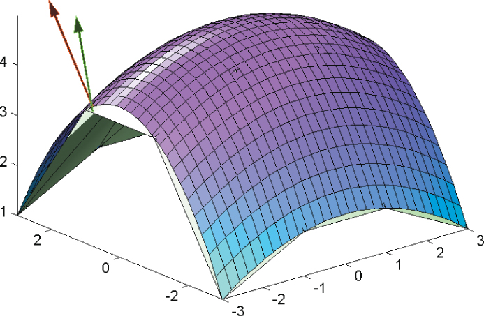
Figure 1.17: A semitransparent smooth surface and a normal vector to it (red), with a polygonal approximation (white) within, and a normal vector to the polygonal mesh at a corresponding point (green).
For a perfectly reflective surface like a mirror (a specular surface), light that arrives10 in a direction ![]() and hits the triangle T is reflected in the
and hits the triangle T is reflected in the ![]() n-plane, with the angle between the outgoing vector and n being the same as the angle between
n-plane, with the angle between the outgoing vector and n being the same as the angle between ![]() and n.
and n.
10. There are two possible choices for describing the light arriving at a surface: Either record the direction of travel of the photons (the transport-centered view), or record the direction from the surface point to the light (the reflection-centered view). For now, we’ll use ![]() for the former; many papers use L for the latter.
for the former; many papers use L for the latter.
For other surfaces, incoming light scatters in many directions.
For completely diffuse surfaces, light scatters in every direction (Figure 1.18) but the brightness of the reflected light varies in proportion to the absolute value of the dot product11 |![]() · n|, that is, the cosine of the angle between the surface normal and the incoming light direction.12 So a surface that faces the light appears bright from wherever one sees it, while a surface that’s tilted a bit away from the light appears dimmer. This kind of scattering was described by Lambert long before the development of computer graphics. As a precondition for scattering, the surface must be facing the light, that is,
· n|, that is, the cosine of the angle between the surface normal and the incoming light direction.12 So a surface that faces the light appears bright from wherever one sees it, while a surface that’s tilted a bit away from the light appears dimmer. This kind of scattering was described by Lambert long before the development of computer graphics. As a precondition for scattering, the surface must be facing the light, that is, ![]() · n < 0. (This Lambertian reflectance model is discussed further in Chapters 6 and 27.)
· n < 0. (This Lambertian reflectance model is discussed further in Chapters 6 and 27.)
11. The dot product is reviewed in Section 7.6.4.
12. This description is so vague that it’s almost meaningless; to make it sensible, we need to discuss how we measure light brightness (a term we’re using informally here), which is quite subtle. For now, you should just imagine that brightness is measured from zero to one in some unstated units.
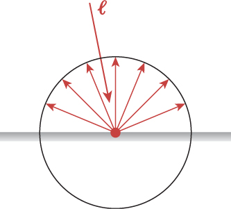
Figure 1.18: Light arrives traveling in direction ![]() ; it’s reflected in all directions. For a source of fixed brightness, the intensity of the reflected light is greatest when
; it’s reflected in all directions. For a source of fixed brightness, the intensity of the reflected light is greatest when ![]() is perpendicular to the surface.
is perpendicular to the surface.
For somewhat shiny surfaces, the appearance of the surface depends on your viewpoint; if you look at a surface in a well-lit room and move your head back and forth, you may see highlights move on the surface. This can be modeled, with an empirically decent fit, by saying that the reflected light is in proportion to (n · h)k for some exponent k, where h is computed from the average of the vector –![]() from the surface to the light and the vector e from the surface to the eye, by adjusting that vector to have unit length, that is:
from the surface to the light and the vector e from the surface to the eye, by adjusting that vector to have unit length, that is:
This model of scattering is due to Phong [Pho75] and Blinn [Bli77], and has been widely used in graphics.
For surfaces in general, the reflected light is a combination of the diffuse, somewhat shiny, and specular cases.
1.13.3. Light Capture
The sensor in a camera and the human eye both respond to light in a similar way: They accumulate light energy for some period of time and then report that accumulated energy. In the case of the sensor, the time period is determined by the shutter opening; in the case of the cell in the eye, the cell sends a signal when the accumulated light reaches some level, so the frequency of signals is proportional to the arriving light intensity. Simulating such a sensor (or cell) therefore involves computing an integral of the incoming light over the area of the sensor. Writing down an analytic solution to this integral for any but the simplest scenes is impractical. For more interesting scenes, we have to perform numerical integration. That necessarily introduces some error, but it also opens up a vast array of computational options for trading quality against time and space. We must approximate the integral by numerical integration, which involves evaluating the integrand at several places (this is called sampling) and then combining these samples to estimate the overall value. The simplest possible version of this approach is to evaluate the incoming light at the sensor center only, and multiply this sample by the area of the sensor to estimate the overall incoming light integral. If the incoming light intensity changes slowly as a function of position, this works quite well; if it changes rapidly, the single-sample approximation introduces many kinds of errors.
1.13.4. Image Display
Modern displays typically are divided into small squares called pixels; each small square13 is individually addressable and can be told to send out a mix of red, green, and blue (RGB) light by specifying a triple of numbers (r, g, b), each between 0 and 255. The amount of light emitted from the square is not directly proportional to the numbers; instead, it follows a relation so that equal differences in numbers correspond approximately to equal differences in perceived brightness. You’ve probably encountered the use of RGB triples in some photo-editing program; typically the RGB values each occupy a single byte, and hence are represented by numbers between 0 and 255, and sometimes are written as two-digit hexadecimals. Thus, a color expressed as 0xFF00CC can be read as “Red is FF, which is 255, there’s no green at all, and there’s CC worth of blue, which is 204 decimal; that means it’s a somewhat reddish purple.” It isn’t obvious what any given color triple or set of hexadecimal values will yield as a hue; color specification is discussed in Chapter 28.
13. The term “pixel” is also used to denote one of the values stored in an image, or a small physical portion of a sensor. There are subtle differences in these denotations, and you should not say “a pixel is a little square” [Smi95].
1.13.5. The Human Visual System
Our eyes respond to light that arrives at the lens, passes through the pupil, and reaches the retina. While direct sunlight is almost 1010 times as bright as the faint light in a dark bedroom, our eyes can detect and process both, but not at the same time. In fact, our eyes adapt to the general illumination around us, and once adapted we can distinguish light intensities that range over a factor of about 1000: The faintest thing we can distinguish from black is presenting light to our eyes that’s about 1/1000 the intensity of the thing we perceive as being “as bright as possible.” Our perception of brightness is not linear, however: If you print thin black stripes on a piece of white paper so that only 20% of the white paper remains visible, it will reflect only 20% of the light that falls on it. But if you place that piece of paper next to a blank piece of the same type of white paper and view both from a distance great enough that the stripes are not visible, the printed paper will appear about half as bright as the unprinted paper. Roughly speaking, for an eye adapted to a given level of light, reducing the incoming light intensity by 80% will make the light seem half as bright.
Our visual system organizes the patterns of light and darkness that arrive at the eye and attempts to make sense of them. The visual system is extremely well adapted to bad input: We can take a black-and-white photograph and add noise (grayscale variation) to it and still be able to recognize the objects in it. We can recognize our homes even in a rainstorm. We can recognize a friend in bright sunlight or in a dark room. In fact, our visual systems are so well tuned to seeing shapes that even when we are watching the static patterns on an old analog television, we occasionally believe we see recognizable patterns. One consequence of this adaptation to bad input is that any stimulus that triggers approximately the right responses leads to recognition: A photograph of a pair of dice, a pencil drawing of them, and a bad computer graphics rendering of them all generate in our brains the perception that we are seeing a pair of dice. This has proved to be a blessing and a curse for the field of computer graphics; it means that even very bad approximations of reality make images that we recognize, so it’s easy to get started in graphics. On the other hand, it’s also easy to believe that the bad approximations are correct because they “look good,” and this can impede progress in the field. The adaptability of the visual system has two effects. First, hacking away at graphics can be very satisfying, because even initial results look good enough, on account of adaptability, to make you believe you’re getting somewhere. And second, results that appear visually very close to perfect may in fact be generated by programs that are not at all correct, because your visual system is hiding errors from you. Hacking away is really fun (and we encourage you to do it at every opportunity), but it may lead you away from your real goal. We have therefore structured this book so that you get the satisfaction of making fairly good pictures right away, but you also learn, as you do so, the limitations of the techniques that you’re learning so that you’re better prepared for the more advanced techniques you’ll encounter later. If you find yourself asking, “But won’t that look wrong in such-and-such a case?” the answer is almost surely “Yes!,” and the later chapters will help you understand how to address these limitations.
To return to the importance of perception, in resource-critical applications an understanding of the perception process lets us make informed decisions about what kinds of approximations we can make while still retaining visual fidelity.
1.13.6. Mathematics
Rather than trying to briefly introduce all the mathematics involved in computer graphics, we’ll introduce the ideas as they arise; most of them are not directly relevant to a basic understanding of graphics, but rather to the efficient representation or approximation of things we use in graphics. However, after giving you a first taste of 2D and 3D graphics in Chapters 2 and 6, we will review in Chapter 7 some of the mathematics that we assume is familiar to our readers, in part to establish the notational conventions that we’ll follow throughout the book. You can write graphics programs with only a knowledge of arithmetic and algebra, but to really work with things in a reasonable way, you’ll want to be familiar with the following:
• Trigonometry
• Operations on small vectors and matrices (which we already discussed in this chapter)
• Integrals and derivatives
• And some geometric and topological notions, like continuity, the geometry of surfaces in three dimensions, and curvature
All of this is made easier by a working knowledge of basic linear algebra, which we assume throughout the book.
1.13.7. Integration and Sampling
The most fully developed area of computer graphics is photorealistic rendering—producing an image from some model of a scene and the lights in it. Each pixel of a rendered image can be thought of as representing a measurement of the light passing along certain rays in the scene, just as each pixel of a digital photograph is a measurement of all the light that hit one small region of the photo sensor in the camera. This can be seen as an integral of the incoming light energy over that region. Since it’s impractical to evaluate most such integrals exactly, we end up using approximations (e.g., the rule we mentioned earlier that states that the “integral is approximately the value at the center of the region, multiplied by the area of the region”). In doing this, we’ve replaced the desired value by a value computed from a single sample; we could have used more samples, but in practice, we’ll always be using a finite number of samples, and using these to estimate some integral. Thus, the process of sampling, and of approximating integrals through samples, is central to rendering.
![]() Every measurement in science is an act of statistics: Our measuring device may function differently from day to day; the thing we measure may be just one of many possible, nearly equivalent, measurements (think of measuring the temperature in a beaker of water; you only really measure it in one part of the beaker). In the case of rendering, the statistic is some integral; the random variable is the set of samples that we use to evaluate it, and the result is that a given rendering of a scene usually depends on some random number generator: Multiple renderings of the same scene with the same software will produce different values for any particular pixel. This distribution of values will typically cluster around some mean value, which one hopes is correct, and will have some variance. If the variance of adjacent pixels is uncorrelated, it may appear in the output as speckle, or visual noise. If it’s correlated, it may appear as jaggies—a staircaselike representation of what should be a smooth diagonal line. This means that assessing the quality of an algorithm also entails statistical measurements.
Every measurement in science is an act of statistics: Our measuring device may function differently from day to day; the thing we measure may be just one of many possible, nearly equivalent, measurements (think of measuring the temperature in a beaker of water; you only really measure it in one part of the beaker). In the case of rendering, the statistic is some integral; the random variable is the set of samples that we use to evaluate it, and the result is that a given rendering of a scene usually depends on some random number generator: Multiple renderings of the same scene with the same software will produce different values for any particular pixel. This distribution of values will typically cluster around some mean value, which one hopes is correct, and will have some variance. If the variance of adjacent pixels is uncorrelated, it may appear in the output as speckle, or visual noise. If it’s correlated, it may appear as jaggies—a staircaselike representation of what should be a smooth diagonal line. This means that assessing the quality of an algorithm also entails statistical measurements.
1.14. Learning Computer Graphics
The subject matter of computer graphics is no longer linearizable in any reasonable way. Each topic ends up so intertwined with all others that there’s no way to decide which one to discuss first, and any presentation ends up with successive disclosures: a first description, a later correction, a further improvement, etc. Readers, naturally, like books to be organized; when you want to review something about polygon meshes, you hope there will be a chapter that has all the polygon-mesh information in it, for instance. Then again, a book that treated each subject in its entirety before moving on to any other would have you make your first pictures at the end of an entire semester of study, at the earliest!
We have compromised: In this introductory chapter, we’ve given you some very informal information about light, perception, the representation of shapes, and the interaction of light with shapes so that you can understand how to make some pictures right away. When you do make pictures with these sloppy models of things, the pictures won’t be very good. Sure, your picture of a boxy robot will be recognizable as a boxy robot, but in looking at it critically, you’ll soon realize that there’s no way you could make a real robot shape (from cardboard, tape, and paint, say) and photograph it with a real camera and end up with anything like the picture you’ve made. It’s not photorealistic. But making those first pictures will give you experience with creating models, with certain applications of linear algebra, with polygonal meshes, and with some key ideas for rendering, all of which will make you better able to understand and experiment with richer or more accurate models of light, reflection, objects, etc., as you encounter them.
The next few chapters introduce Microsoft’s Windows Presentation Foundation (WPF), a framework for writing graphics programs, some basic ideas from rendering, an introduction to visual perception, and quite a lot of mathematics that’s useful throughout graphics.
Chapter 2 introduces the 2D aspects of WPF to get you familiar with drawing simple 2D shapes. WPF uses a declarative specification of graphics—in contrast to more traditional APIs—which is valuable both because it provides a higher level of abstraction and because its interpretive nature makes it very useful for rapid prototyping. Modeling in WPF is based on a hierarchical representation of shapes that’s widely used in almost all graphics APIs.
Chapter 3 describes a program for making very simple pictures of very simple 3D shapes so that you can understand from the start how simple graphics can be. Chapter 4 describes two WPF programs that you’ll use when conducting experiments in graphics throughout much of the remainder of the book.
Chapter 5, which covers perception, describes some of the most pertinent aspects of the human visual system.
In Chapter 6 we present an introduction to the 3D aspects of WPF, which also informally introduces the geometric tools used for shape modeling, and the application of the simple models of how light and objects interact that we have described in this chapter. It also continues the description of hierarchical models of compound shapes introduced in Chapter 2.
With the experience of using both the 2D and 3D versions of WPF, you will be prepared for Chapter 7’s review of mathematical essentials for graphics. Chapters 8 through 13 introduce the linear algebra that lies at the core of a great deal of computer graphics, together with certain data structures that represent the topology and geometry from which we make images.
Following this, we again discuss (in Chapter 14) the conventional approximations to reality—the models—that are used in many basic graphics systems. We describe models of light, of shape, of material, and of how light is transported in a scene, in each case with more detail than in this chapter. This rather long chapter not only prepares you for the later material on rendering, shape representation, and material representation, but also introduces many topics that are essential for understanding legacy programs.
With an understanding of basic models of light and reflection, we can make preliminary versions of two renderers: a ray tracer and a rasterizer (Chapter 15). Doing so introduces the key ideas and challenges of each kind of rendering; because our preliminary versions are so basic, Chapter 15 also introduces some of the problems of each, and of the conventional approximations to reality.
In Chapter 16 we discuss various graphics systems, comparing and contrasting them with WPF; by the end of that chapter, you will have encountered much of what was traditionally taught in computer graphics.
The remaining chapters in the book discuss images and signal processing, light, color, materials, texturing, and rendering; cover some interaction techniques, geometric algorithms and data structures that support rendering as well as many interaction methods, and various approaches to modeling shapes; and introduce animation and graphics hardware. These chapters are less sequential and more interdependent than the chapters preceding them. You can skip forward and read about splines and subdivision surfaces if you want to learn how to create interesting shapes, but you’ll find references to the ideas of convolution and filtering that were introduced in Chapters 17 through 19. You can read about some of the best available rendering algorithms in Chapter 32, but you’ll find that the discussion relies heavily on the discussion of rendering theory in Chapter 31. This should not prevent you from taking this approach; for many students, it’s the desire to make the practical algorithms work that motivates them to learn more about the theory, and if you read Chapter 31 with particular questions in mind, you may find the material easier to absorb.