
Chapter 31. Computing Solutions to the Rendering Equation: Theoretical Approaches
31.1. Introduction
In this chapter we discuss the theory of solving the rendering equation, concentrating on the mathematics of various approaches and on what kinds of approximations are involved in these approaches, deferring the implementation details to the next chapter. Fortunately, much of the mathematics can be understood by analogy with far simpler problems. When we render, we’re trying to compute values of L, the radiance field, or expressions involving combinations (typically integrals) of many values of L. Thus, the unknown is the whole function L. That’s in sharp contrast to the equations like
that we see in algebra class, where the unknown, x, is a single number. Nonetheless, such simple equations provide a useful model for the approximations made in the more complicated task of finding L; we discuss these first, and then go on to apply these ideas to rendering.
31.2. Approximate Solutions of Equations
There’s no hope of solving the rendering equation exactly for any scene with even a moderate degree of complexity. Instead, we are forced to approximate solutions. There are four common forms of approximation that are routinely used in graphics:
• Approximating the equation
• Restricting the domain
• Using statistical estimators
• And bisection/Newton’s method
Because the last of these is not used much in rendering, it’ll get brief treatment. The statistical approach, however, which now dominates rendering, will occupy much of the rest of the chapter.
We’ll discuss these in the context of a much simpler problem: Find a positive real number x for which
The numerical solution of this equation is x = 0.5265 ..., but let’s pretend that we don’t know that, and we’re restricted to computations easily done by hand, like addition, subtraction, multiplication, division, and finding integer powers of a real number.
31.3. Method 1: Approximating the Equation
Instead of solving 50x2.1 = 13, which would involve the extraction of a 2.1th root, we could solve a “nearby” equation like
which simplifies to ![]() , and get the answer x = 0.5. Since multiplication and exponentiation are both continuous, it should be no surprise that the solution to this slightly “perturbed” equation is quite close to the solution of the original (see Figure 31.1). Solving the perturbed equation is easy.
, and get the answer x = 0.5. Since multiplication and exponentiation are both continuous, it should be no surprise that the solution to this slightly “perturbed” equation is quite close to the solution of the original (see Figure 31.1). Solving the perturbed equation is easy.
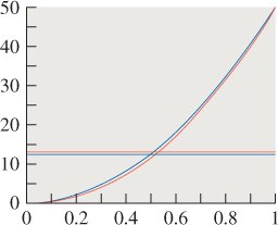
Figure 31.1: The graph of y = 50x2 (blue) is very close to that of y = 50x2.1 (just below it, in red); the x-coordinate of the intersection of the blue graph with the line y = 12.5 is very near that of the red graph with the line y = 13.
You might well complain that the word “nearby” was left undefined in the preceding paragraph. As a different example, consider solving
for x. The solution is x = 105. But if we alter the equation just a little, making the right-hand side 0 instead of 0.1, the solution becomes x = 0: A small perturbation in the equation led to a huge perturbation in the solution. Determining the sensitivity of the solution to perturbations in the equation is (for more complicated equations like the rendering equation) often extremely difficult; in practice, it’s done by saying things like, “It seems pretty obvious that the moonlight coming through my closed bedroom curtains wouldn’t look very different if the moon were oval rather than round.” In other words, it’s done by using domain expertise to decide which kinds of approximations are likely to produce only minor perturbations in the results.
An example of this in rendering is the approximation of reflection from an arbitrary surface by the Lambert reflection model, or the approximation of the “Is that light source visible from this point?” function, by the function that always says “yes.” The first leads to solutions where nothing looks shiny, and the second leads to solutions where there are no shadows; each is often a better approximation than an all-black image, and a poor approximation is frequently better than no solution at all.
31.4. Method 2: Restricting the Domain
Instead of trying to find a positive real number x satisfying
we can ask, “Is there a positive integer satisfying (or nearly satisfying) it?” (See Figure 31.2.) Such a domain restriction can simplify things enormously. In the case of this equation, we see that the left-hand side is an increasing function of x, and that when x = 1, its value is already 50. So any integer solution must lie between zero and one. We need only try these two possible solutions to see which one works (or, if none works, which is “best”). We quickly find that x = 0 gives 50x2.1 = 0, which is too small, and x = 1 gives 50, which is too large.
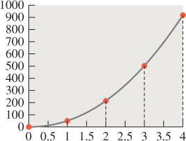
Figure 31.2: The graph of y = 50x2.1, restricted to x = 0, 1, 2, 3, 4, shown as a stem plot with small red circles, atop the graph on the whole real line (shown in gray).
We then have two choices: We can report the “best” solution in the restricted domain (x = 0), or we can perhaps say, “The ideal solution lies somewhere between 0 and 1, much closer to 0 than to 1; linear interpolation gives x = 0.26 as a best-guess answer.” (See Figure 31.3.)
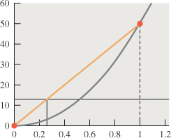
Figure 31.3: Because the value at x = 0 is too small, and at x = 1 it’s too large, we estimate the solution x by intersecting the connect-the-dots plot (orange) with the line y = 13 to get x = 0.26.
Our use of linear interpolation incorrectly assumes that the values of the left-hand side F(x) = 50x2.1 vary almost linearly as a function of x between x = 0 and x = 1, which is why the estimated answer isn’t very close to the true one. More generally, if the domain of some variable is D, and we restrict to a subset D′ ![]() D, then estimating a solution in D from approximate solutions in D′ requires that D′ is “large enough” that any point d of D lies near enough to points of D′ that F(d) can be well inferred from values of F at nearby points of D′.
D, then estimating a solution in D from approximate solutions in D′ requires that D′ is “large enough” that any point d of D lies near enough to points of D′ that F(d) can be well inferred from values of F at nearby points of D′.
We’ll see an example of domain restriction in rendering when we discuss radiosity. Note that methods 1 and 2 both violate the Approximate the Solution principle: they approximate the problem rather than the solution.
31.5. Method 3: Using Statistical Estimators
A third approach is to “estimate” the solution statistically, that is, find a way to produce a sequence of values x1, x2, ... such that each xi is a possible solution, and such that the average an of x1, x2, ..., xn gets closer and closer to a solution as n gets large.
In this case, we’re trying to solve
whose solution is
This can be easily evaluated on a computer, but we’re assuming we lack the ability to compute anything more complicated than an integer power of a real number. (When we look at the rendering equation, the corresponding statement will be, “Suppose we lack the ability to compute anything except an integral number of bounces of a ray of light,” which is very reasonable: It’s hard to imagine what it might mean to compute 2.1 bounces of a light ray!) We can still find a solution using the binomial theorem, which says that
where
is defined for any real number α and for k = 0, 1, .... We’ll be applying this to the case ![]() and
and ![]() , so that
, so that ![]() , so that evaluating Equation 31.8 will give us the value of the solution in Equation 31.7.
, so that evaluating Equation 31.8 will give us the value of the solution in Equation 31.7.
To do so requires summing an infinite series, however. The great insight is the realization that the sum of an infinite series can be estimated by looking at individual elements of the series.
31.5.1. Summing a Series by Sampling and Estimation
We now lay the foundations for all the Monte Carlo approaches to rendering, starting with a few simple applications of probability theory.
31.5.1.1. Finite Series
Suppose that we have a finite series
and we want to estimate the sum, A. We can do the following: Pick a random integer i between 1 and 20 (with probability 1/20 of picking each possible number), and let X = 20ai. Then X is a random variable. Its expected value is the weighted average of its values, with weights being the probabilities, that is,
We’ve got a random variable whose expected value is the sum we’re seeking! By actually taking samples of this random variable and averaging them, we can approximate the sum.
Suppose that all 20 numbers a1, a2, ... are equal. What’s the variance of the random variable X? How many samples of X do you need to take to get a good estimate of A in this case?
In general, the variance of X is related to how much the terms in the sequence vary: If all the terms are identical, then X has no variance, for instance. It’s also related to the way we chose the terms, which happens to have been uniform, but we’ll use nonuniform samples in other examples later. When we apply these ideas to rendering, we will end up sampling among various paths along which light can travel; the value being computed will be the light transport along the path. Since some paths carry a lot of light (e.g., a direct path from a light source to your eye) and some carry very little, a large variance is present; to make estimates accurate will require lots of samples, or some other approach to reducing variance. For a basic ray tracer, this means you may need to trace many rays per pixel to get a good estimate of the radiance arriving at a single image pixel.
31.5.1.2. Infinite Series
It’s tempting to generalize to infinite series A = a1 + a2 + ... in the obvious way: Pick a non-negative integer i, and let X = ai; make all choices of i equally probable, and then the expected value of X should be A. There are two problems with this, however. First, there’s the missing factor of 20. In the finite example, we multiplied each ai by 20 because the probability of picking it was 1/20. This means that in the infinite case, we’d need to multiply each ai by infinity, because the probability of picking it is infinitesimal. This doesn’t make any sense at all. Second, the idea of picking a positive integer uniformly at random sounds good, but it’s mathematically not possible. We need a slightly different approach, motivated by Equation 31.11, in which each term of the series is multiplied by the probability of picking that term (1/20) and by the inverse of that probability (20). All we need to do is abandon the idea of a uniform distribution.
To sum the series
we can pick a non-negative integer j with probability 1/2j so that the probability of picking j = 1 is 1/2 and the probability of picking j = 10 is 1/210 = 1/1024. (This particular choice of probabilities was made because it’s easy to work with, and it’s obvious that the probabilities sum to 1, but any other collection of positive numbers that sum to 1 would work equally well.)
We then let
Just as before, the expected value of X is
And just as before, the variance in the estimate is related to the terms of the series. If aj happens to be 2-j, then the variance is zero and the estimator is great. If aj = 1/j2, then the variance is considerably larger, and we’ll need to average lots of samples to get a low-variance estimate of the result.
As we said, the particular choice we made in picking j—the choice to select j with probability 2-j—was simple, but we could have used some other probability distribution on the positive integers; depending on which distribution we choose, the estimator may have lower or higher variance.
When it comes to applying this approach to rendering, the choice of j will become the choice of “how many bounces the light takes.” If we have a scene in which the albedo of every surface is about 50%, then we expect only about half as much light to travel along paths of length k + 1 as did along paths of length k.
In this case, assigning half the probability to each successive path length makes some sense. In general, picking the right sampling distribution is at the heart of making such Monte Carlo approaches work well.
31.5.1.3. Solving 50x2.1 = 13 Stochastically
Applying these methods to our particular equation, we know that
and that in general we can transform the right-hand side of the equation using the binomial theorem
Doing so, with ![]() and
and ![]() , we get
, we get
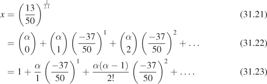
Now, to estimate a solution, we pick a positive integer j with probability 2–j, and evaluate the jth term. As we wrote this chapter, we flipped coins and counted the number of flips until heads, generating the sequence 3, 3, 1; our three estimates of x are thus the third, third, and first terms of the series, multiplied by 8, 8, and 2, respectively:
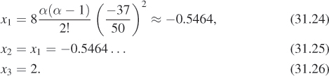
Recall that the correct solution to the problem is 0.5265. The average of our three samples is x = .3024, which admittedly is not a very good estimate of the solution. When we used 10,000 terms, the estimate was 0.5217, which is considerably closer (see Figure 31.4).
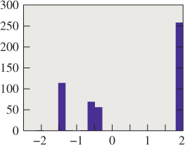
Figure 31.4: A histogram of 500 estimates of the root of 50x2.1 = 13; their average is quite near 0.5625.
You may be concerned that we’ve assumed we can write a power series for x, but that when we get to the rendering equation, such a rewrite may not be so easy. Fortunately, in the case of the rendering equation, the rewrite as an infinite series is actually quite easy, although estimating the sum of the resultant series still involves the same randomized approaches.
31.6. Method 4: Bisection
Our final approach to solving the equation is to find a value of x for which 50x2.1 is less than 13 (such as x = 0) and one for which it’s greater than 13 (such as x = 1). Since f(x) = 50x2.1 is a continuous function of x, it must take on the value 13 somewhere between x = 0 and x = 1. We can evaluate ![]() and find that it’s less than 13; we now know that the solution’s between
and find that it’s less than 13; we now know that the solution’s between ![]() and 1. Repeatedly evaluating f at the midpoint of an interval that we know contains the answer, and then discarding half the interval on the basis of the result, rapidly converges on a very small interval that must contain the solution.
and 1. Repeatedly evaluating f at the midpoint of an interval that we know contains the answer, and then discarding half the interval on the basis of the result, rapidly converges on a very small interval that must contain the solution.
This can be seen as a kind of binary search on the real line. There are also “higher order” methods, like Newton’s method, in which we start at some proposed solution x0 and say, “If f were linear, then we could write it as y = f(x0) + f′(x0)(x – x0).” But that function is zero at ![]() . So let’s evaluate f at x1 and see whether it’s any smaller there, and iterate. If x0 happens to be near a root of f, this tends to converge to a root quite fast. If it’s not (or if f′(x0) = 0), then it doesn’t work so well.
. So let’s evaluate f at x1 and see whether it’s any smaller there, and iterate. If x0 happens to be near a root of f, this tends to converge to a root quite fast. If it’s not (or if f′(x0) = 0), then it doesn’t work so well.
Despite the appeal of these approaches, there’s no easy analog in the case of functional equations (ones where the answer is a function rather than a number) like the rendering equation. There’s no simple way to generalize the notion of one number being between two others to the more general category of functions.
Nonetheless, bisection gets used a lot in graphics, and these four approaches to solving equations serve as archetypes for solving equations throughout the field.
31.7. Other Approaches
There are other approaches to equations that cannot be easily illustrated with our 50x2.1 = 13 example. For instance, you might say, “I can solve systems of two linear equations in two unknowns ...but only if the coefficients are integers rather than arbitrary real numbers.” In doing so, you’re not really solving the general problem (“two linear equations in two unknowns”), but it may be that the subclass of problems you can solve is interesting enough to merit attention. In graphics, for instance, early rendering algorithms could only work with a few point lights rather than arbitrary illumination; some later algorithms could only work on scenes where all surfaces were Lambertian reflectors, etc.
As a second example, you may arrive at a method of solution that’s too complex, and choose to approximate the method of solution rather than the original equation. For instance, the Monte Carlo approach used to sum an infinite series above might seem overly complicated, and you might choose to just sum the first four terms. This sounds laughable, but in practice it can often work quite well. Most basic ray tracers, for instance, trace secondary rays only to a predetermined depth, which amounts to truncating a series solution after a fixed number of terms.
31.8. The Rendering Equation, Revisited
Recall that a radiance field is a function on the set ![]() of all surface points in our scene, and that it takes a point, P
of all surface points in our scene, and that it takes a point, P ![]()
![]() , and a direction, ω, and returns a real number indicating the radiance along a ray leaving P in direction ω. Our model of the radiance field is a function L :
, and a direction, ω, and returns a real number indicating the radiance along a ray leaving P in direction ω. Our model of the radiance field is a function L : ![]() × S2
× S2 ![]() R.
R.
There is a subtlety here that we discussed in Section 29.4: There are some “sur-face points” that are part of two surfaces. For instance, if we have a solid glass sphere (see Figure 31.5), the point at the north pole of the sphere is really best thought of as two points: one on the “outside” and the other on the “inside.” Light traveling northward at the outer point is either reflected or transmitted, while light traveling northward at the inner point is arriving there and is about to be transmitted or reflected by the glass-air interface. As we suggested, we can enhance the notion of the light field to take three arguments—a point, a direction, and a normal vector that defines the “outside” for this point—but in the remainder of this chapter, we’re going to instead discuss only reflection (except at a few carefully indicated points), since (a) the two-points-in-one-place idea complicates the notation, which is complex enough already, and (b) the actual changes in the programs that we’ll see in Chapter 32 to account for transmission are relatively minor and straightforward. As for the matter of keeping two separate copies of the north pole, in practice, as we’ll discuss in Chapter 32, we’ll only keep a single copy of the geometry, and there will be no explicit representation of the light field; on the other hand, the meaning of an arriving light ray, and how it is treated, will depend on the dot product of its direction with the unit normal n, resulting in several if-else clauses in our programs.
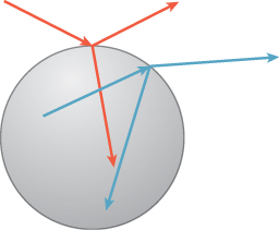
Figure 31.5: Light from above the sphere both reflects and refracts, as does light in the inside of the sphere.
We’ll continue to write fs for the scattering function, however, but you’ll need to remember that in the case of transmission, some ω · n terms may need absolute-value signs on them.
The rendering equation characterizes the radiance field (P, ω) ![]() L(P, ω) in a scene by saying that the radiance at some surface point, in some direction, is a sum of (a) the radiance emitted at that point in that direction, and (b) all the incoming light at that point that is scattered in that direction. This equation has the form
L(P, ω) in a scene by saying that the radiance at some surface point, in some direction, is a sum of (a) the radiance emitted at that point in that direction, and (b) all the incoming light at that point that is scattered in that direction. This equation has the form
Recall the meaning of the terms:
• E is the emitted radiance field, with E(P, ω) = 0 unless P is a point of some luminaire, and ω is a direction in which that luminaire emits light from P.
• T(L) is the scattered radiance field due to L;T(L)(P, ωo) is the light scattered from the point P in the direction ωo when the radiance field for the whole scene is L.1
1. We use the letter T rather than S (for “scattering”) because S will be used later in describing various light paths.
To be specific, T is defined by
The critical feature of this expression, for our current discussion, is that L appears in the integral.
Note that if we solve Equation 31.27 for the unknown L, we don’t yet have a picture! We have a function, L, which can be evaluated at a bunch of places to build a picture. In particular, we might evaluate L(P, ω) for each pixel-center P and the corresponding vector ω from the pinhole of a pinhole camera through P (assuming a physical camera, in which the film plane is behind the pinhole).
What are the domain and codomain of T? In other words, what sort of object does T operate on, and what sort of result does it produce? The answer to the latter question is not “It produces real numbers.”
![]() The function T is a higher-order function: It takes in functions and produces new functions. You’ve seen other such higher-order functions, like the derivative, in calculus class, and perhaps have encountered programming languages like ML, Lisp, and Scheme, in which such higher-order functions are commonplace.
The function T is a higher-order function: It takes in functions and produces new functions. You’ve seen other such higher-order functions, like the derivative, in calculus class, and perhaps have encountered programming languages like ML, Lisp, and Scheme, in which such higher-order functions are commonplace.
![]() Let’s consider this integral from the computer science point of view. We have a well-defined problem we want to solve (“find L”), and we can examine how difficult a problem this is. First, for even fairly trivial scenes, it’s provable that there’s no simple closed-form solution. Second, observe that the domain of L is not discrete, like most of the things we see in computer science, but instead is a rather large continuum—there are three spatial coordinates and two direction coordinates in the arguments to L, so it’s a function of five real variables. (Note: In graphics, it’s common to call this a “five-dimensional function,” but it’s more accurate to say that it’s a function whose domain is five-dimensional.) In computer science terminology, we’d call a classic problem like a traveling salesman problem or 3-SAT “difficult,” because the only known way to solve such a problem is no simpler, in big-O terms, than enumerating all potential solutions. By comparison, because of the continuous domain, the rendering equation is even harder, because it’s infeasible even to enumerate all potential solutions. Your next thought may be to develop a nondeterministic approach to approximate the solution. That’s a good intuition, and it’s what most rendering algorithms do. But unlike many of the nondeterministic algorithms you’ve studied, while we can characterize the runtime of these randomized graphics algorithms, that in itself isn’t meaningful, because the errors in the approximation are unbounded in the general case: Because the domain is continuous, and we can only work with finitely many samples, it’s always possible to construct a scene in which all the light is carried by a few sparse paths that our samples miss.
Let’s consider this integral from the computer science point of view. We have a well-defined problem we want to solve (“find L”), and we can examine how difficult a problem this is. First, for even fairly trivial scenes, it’s provable that there’s no simple closed-form solution. Second, observe that the domain of L is not discrete, like most of the things we see in computer science, but instead is a rather large continuum—there are three spatial coordinates and two direction coordinates in the arguments to L, so it’s a function of five real variables. (Note: In graphics, it’s common to call this a “five-dimensional function,” but it’s more accurate to say that it’s a function whose domain is five-dimensional.) In computer science terminology, we’d call a classic problem like a traveling salesman problem or 3-SAT “difficult,” because the only known way to solve such a problem is no simpler, in big-O terms, than enumerating all potential solutions. By comparison, because of the continuous domain, the rendering equation is even harder, because it’s infeasible even to enumerate all potential solutions. Your next thought may be to develop a nondeterministic approach to approximate the solution. That’s a good intuition, and it’s what most rendering algorithms do. But unlike many of the nondeterministic algorithms you’ve studied, while we can characterize the runtime of these randomized graphics algorithms, that in itself isn’t meaningful, because the errors in the approximation are unbounded in the general case: Because the domain is continuous, and we can only work with finitely many samples, it’s always possible to construct a scene in which all the light is carried by a few sparse paths that our samples miss.
![]() One strategy for generating approximate solutions is to discretize the domain in some way so that we can bound the error. That’s also a good idea, because we might then be able to enumerate some sizable portion of the solution space. I can’t look at light transport for every point on a curved surface, but I can look at it for every vertex of a triangle-mesh approximation of that surface. Graphics isn’t unique in this. The moment you take computer science out of pure theory and start applying it to physics, you’ll find that problems are often of more than exponential complexity, and you often need to find good approximations that work well on the general case, even if you can’t bound the error in all cases.
One strategy for generating approximate solutions is to discretize the domain in some way so that we can bound the error. That’s also a good idea, because we might then be able to enumerate some sizable portion of the solution space. I can’t look at light transport for every point on a curved surface, but I can look at it for every vertex of a triangle-mesh approximation of that surface. Graphics isn’t unique in this. The moment you take computer science out of pure theory and start applying it to physics, you’ll find that problems are often of more than exponential complexity, and you often need to find good approximations that work well on the general case, even if you can’t bound the error in all cases.
Recall from Chapter 29 the division of light in a scene into two categories (see Figure 31.6): At a point of a surface, light may be arriving from various points in the distance, a condition called field radiance. This light hits the surface and is scattered; the resultant outgoing radiance is called surface radiance.
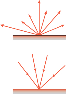
Figure 31.6: Top: The surface radiance consists of all the light leaving a point of a surface. Bottom: The field radiance consists of all the incoming light.
It’s also helpful to divide radiance even further: The surface radiance at a point P can be divided into the emitted radiance there (nonzero only at luminaires) and the reflected radiance. These correspond to the two terms on the right-hand side of the rendering equation. Dually, the field radiance at P can be divided into direct lighting, Ld(P, ω) at P (i.e., radiance emitted by luminaires and traveling through empty space to P), and indirect lighting, Li(P, ω) at P (i.e., radiance from a point Q to a point P along the ray P – Q, but that was not emitted at Q). We’ll return to these terms in the next chapter.
Suppose that P and Q are mutually visible. How are the emitted and reflected radiance at Q, in the direction P – Q, related to the direct and indirect light at P, in the direction P – Q? Express these in terms of Ld, Li, Lr, and Le, being careful about signs. Use ω = S(P – Q) in expressing your answer.
Writing the rendering equation in the form of Equation 31.27 makes it clear that the scattering operator transforms one radiance field (L) into another (T(L)). Not only does it do so, but it does so linearly: If we compute T(L1 + L2), we get T(L1) + T(L2), and T(rL) = rT(L) for any real number r, as you can see from Equation 31.28. This linearity doesn’t arise from some cleverness in the formulation of the rendering equation. It’s a physically observable property, commonly called the principle of superposition in physics, and it’s extremely fortunate, for those hoping to solve the rendering equation, that it holds. Later, in Chapter 35, we’ll see this principle of superposition applying to forces and velocities and other things that arise in physically based animations, and once again it will simplify our work considerably.
We can rewrite the rendering equation in the form
or even
where I denotes the identity operator: It transforms L into L, and we’ve used TL to denote the application of the operator T to the radiance field L.
Much of the remainder of this chapter describes approaches to solving this equation. Remember as we examine such approaches that Le, the light emitted by each light source, is given as an input, as is the bidirectional reflectance distribution function (BRDF) at each surface point, so that the operator T can be computed. The unknown is the radiance field, L.
![]() The similarity of this formulation to the way eigenvalue problems are described in linear algebra is no coincidence. We’ll use many of the same techniques that you saw in studying eigenvalues as we look at solving the rendering equation.
The similarity of this formulation to the way eigenvalue problems are described in linear algebra is no coincidence. We’ll use many of the same techniques that you saw in studying eigenvalues as we look at solving the rendering equation.
31.8.1. A Note on Notation
We summarize in Table 31.1 the notation we’ll use repeatedly throughout this chapter. Figure 31.7 gives the geometric situation to which items in this table refer.
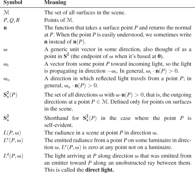
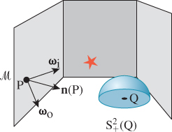
Figure 31.7: Some standard notation. The vector ωi points toward the light source (indicated by a star).
Notice that the subscript “i” in ωi is set in Roman font rather than italics; that’s to indicate that it’s a “naming-style” subscript (like VIN to denote input voltage) rather than an “indexing-style” subscript (like bi, denoting the ith term in a sequence).
When we aggregate over λ, it’s important to decide once and for all whether this aggregate denotes a sum (perhaps an integral from λ = 400 nm to 750 nm), or an average; you can do either one in your code, but you must do it consistently.
Occasionally we will have several incoming vectors at a point P, and we’ll need to index them with names like ω1, ω2, .... When we want to refer to a generic vector in this list, we’ll use ωj, avoiding the subscript i to prevent confusion with the previous use. You will have to infer, from context, that these vectors are all being used to describe incoming light directions, that is, serving in the role of ωi.
As we discussed in Chapter 26, many terms, and associated units, are used to describe light. In an attempt to avoid problems, we’ll use just a few: power (in watts), flux (in watts per square meter), radiance (in watts per square meter steradian), and occasionally spectral radiance (in watts per square meter steradian nanometer).
31.9. What Do We Need to Compute?
Much of the work in rendering falls into a few categories:
• Developing data structures to make the ray-casting operation fast, which we discuss in Chapter 36
• Choosing representations for the function fs that are general enough to capture the sorts of reflectivity exhibited by a wide class of surfaces, yet simple enough to allow clever optimizations in rendering, which we’ve already seen in Chapter 27
• Determining methods to approximate the solution of the rendering equation
It is this last topic that concerns us in this chapter.
The rendering equation characterizes the function L that describes the radiance in a scene. Do we really need to know everything about L? Presumably radiance that’s scattered off into outer space (or toward some completely absorbing surface) is of no concern to us—it cannot possibly affect the picture we’re making. In fact, if we’re trying to make a picture seen from a pinhole camera whose pinhole is at some point C, the only values we really care about computing are of the form L(C, ω). To compute these we may need to compute other values L(P, η) in order to better estimate the values we care about.
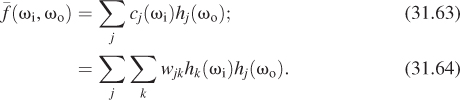
Suppose, however, that we want to simulate an actual camera, with a lens and with a sensor array like the CCD array in many digital cameras. To compute the sensor response at a pixel P, we need to consider all rays that convey light to P—rays from any point of the lens to any point of the sensor cell corresponding to P (see Figure 31.8).
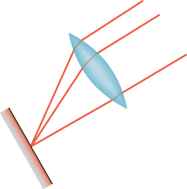
Figure 31.8: Light along any ray from the lens to the sensor cell contributes to the measured value at that cell.
As we said in Chapter 29, light arriving along different rays may have different effects: Light arriving orthogonal to the film plane may provoke a greater response than light arriving at an angle, and light arriving near the center of a cell may matter more than light arriving near an edge—it all depends on the structure of the sensor. The measurement equation, Equation 29.15, says that
where Mij is a sensor-response function that tells us the response of pixel (i, j) to radiance along the ray through P in direction –ω.
One perfectly reasonable idealization is that the pixel area is a tiny square, and that Mij is 1.0 for any ray through the lens that meets this square, and 0 otherwise. Even with this idealization, however, the pixel value that we’re hoping to compute is an integral over the pixel area and the set of directions through the lens. Even if we assume a lens so tiny that the latter integral can be accurately estimated by a single ray (the pinhole approximation), there’s still an area integral to estimate.
One very bad way to estimate this integral is with a single sample, taken at the center of the pixel region (i.e., the simplest ray-tracing model, where we shoot a ray through the pixel center). What makes this approach particularly bad are aliasing artifacts: If we’re making a picture of a picket fence, and the spacing of the pickets is slightly different from the spacing of the pixels, the result will be large blocks of constant color, which the eye detects as bad approximations of what should be in each pixel (see Figure 31.9).
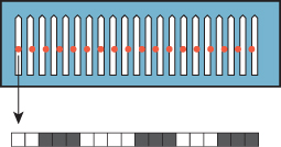
Figure 31.9: Pixel-center samples of a picket-fence scene lead to large blocks of black-and-white pixels.
If we instead take a random point in each pixel, then this aliasing is substantially reduced (see Figure 31.10). Instead, we see salt-and-pepper noise in the image.

Figure 31.10: Random ray selection within each pixel reduces aliasing artifacts, but replaces them with noise.
Because our visual system does not tend to see “edges” in such noise, but is very likely to see incorrect edges in the aliased image, the tradeoff of aliases for noise is a definite improvement (see Figure 31.11).
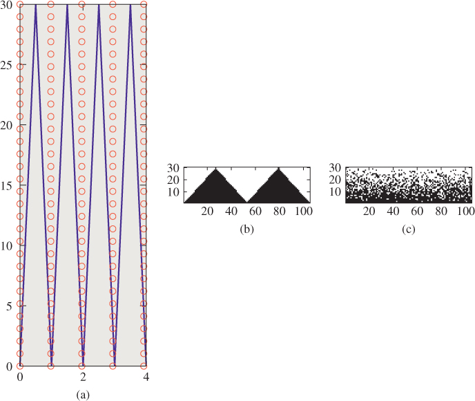
Figure 31.11: (a) A close-up view of a portion of a sawtooth-shaped geometry (note that each sawtooth occupies a little more than one unit on the x-axis) and the locations of pixel samples (small circles). (b) The resultant image. Even though there are 102 teeth in this 104-pixel-wide image, aliasing causes us to see just two. (c) When we take “jittered samples” (each sample is moved up to a half pixel both vertically and horizontally), the resultant image is noisy, but exhibits no aliasing.
This notion of taking many (randomized) samples over some domain of integration and averaging them applies in far more generality. We can integrate over wavelength bands (rather than doing the simpler RGB computations that are so common, which amount to a fixed-sample strategy). We can integrate over the lens area to get depth-of-field effects and chromatic aberration. For a scene that’s moving, we can simulate the effect of a shutter that’s open for some period of time by integrating over a fixed “time window.” All of these ideas were described in a classic paper by Cook et al. [CPC84], which called the process distributed ray tracing. Because of possible confusion with notions of distributed processing, we prefer the term distribution ray tracing which Cook now uses to describe the algorithm [Coo10]. We’ll discuss the particular sampling strategies used in distribution ray tracing in Chapter 32.
In short: To render a realistic image in the general case, we need to average, in some way, many values, each of which is L(P, ω) for some point P of the image plane and some direction ω ![]() S2.
S2.
31.10. The Discretization Approach: Radiosity
We’ll now briefly discuss radiosity—an approach that produces renderings for certain scenes very effectively—and then return to the more general scenes that require sampling methods and discuss how to effectively estimate the value L(P, ω) in the algorithms that work on those scenes.
The radiosity method for rendering differs from the methods we’ve seen in Chapter 15; in those methods, we started with the imaging rectangle and said, “We need to compute the light that arrives here, so let’s cast rays into the scene and see where they hit, and compute the light arriving at the hit point by various methods.” Whether we did this one pixel at a time or one light at a time or one polygon at a time was a matter of implementation efficiency. The key thing is that we said, “Start from the imaging rectangle, and use that to determine which parts of the light transport to compute.” A radically different approach is to simulate the physics directly: Start with light emitted from light sources, see where it ends up, and for the part that ends up falling on the imaging rectangle, record it. This approach was taken by Appel [App68], who cast light rays into the scene and then, at the image plane location of the intersection point (if it was visible), drew a small mark (a “+” sign). In areas of high illumination there were many marks; in areas of low illumination, almost none. By taking a black-and-white photograph of the result (which was drawn with a pen on plotter paper) and then examining the negative for the photograph, he produced a rendering of the incident light.
Radiosity takes a similar approach, concentrating first on the light in the scene, and only later on the image produced. Because the surfaces in the scene are assumed Lambertian, the transformation from a representation of the surface radiance at all points of the scene to a final rendering is relatively easy.
The radiosity approach has two important characteristics.
• It’s a solution to a subproblem, in the sense that it only applies to Lambertian reflectors, and is generally applied to scenes with only Lambertian emitters.
• It’s a “discretization” approach: The problem of computing L(P, ωo) for every P ![]()
![]() and
and ![]() is reduced to computing a finite set of values. The scene is partitioned into small patches, and we compute a radiosity value for each of these finitely many patches.
is reduced to computing a finite set of values. The scene is partitioned into small patches, and we compute a radiosity value for each of these finitely many patches.
The division into patches means that radiosity is a finite element method, in which a function is represented as a sum of finitely many simpler functions, each typically nonzero on just a small region. (The word “finite” here is in contrast to “infinitesimal”: Rather than finding radiance at every single point of the surface, each point being “infinitesimal,” we compute a related value on “finite” patches.)
Radiosity was the first method to produce images exhibiting color bleeding (in which a red wall meeting a white ceiling could cause the ceiling to be pink near the edge where they meet), and not requiring an “ambient term” in its description of reflection—a term included in scattering models (see Chapter 27) to account for all the light in a scene that wasn’t “direct illumination,” which had presented problems for years previously. Figure 31.12 shows an example.
Figure 31.12: A radiosity rendering of a simple scene. Note the color-bleeding effects. (Courtesy of Greg Coombe, “Radiosity on graphics hardware” by Coombe, Harris and Lastra, Proceedings of Graphics Interface 2004.)
The first step in radiosity is to partition all surfaces in the scene into small (typically rectangular) patches. The patches should be small enough that the illumination arriving at a patch is roughly constant over the patch so that the light leaving the patch will be too, and hence can be represented by a single value. This “meshing” step has a large impact on the final results, which we’ll discuss presently. For now, let’s just assume the scene surfaces are partitioned into many small patches. We’ll use the letters j and k to index the patches, and use Aj to indicate the area of patch j, Bj to denote a value proportional to the radiance leaving any point of patch j, in any outgoing direction2 ωo, and nj to indicate the normal vector at any point of patch j.
2. By “outgoing direction,” we mean that ωo · nj > 0; the radiance is independent of direction because the surfaces are assumed Lambertian.
Each patch j is assumed to be a Lambertian reflector, so its BRDF is a constant function,
where ρj is the reflectivity and P is any point of the patch. Furthermore, each luminaire is assumed to be a “Lambertian” emitter of constant radiance, that is, Le(P, ωo) is a constant for P in patch j and ωo an outgoing vector at P.
This simple form for scattering and the assumption about constant emission together mean that the rendering equation can be substantially simplified.
For the moment, let’s make four more assumptions. The first is that the scene is made up of closed 2-manifolds, and no 2-manifold meets the interior of any other (e.g., two cubes may meet along an edge or face, but they may not interpenetrate). This also means that we don’t allow two-sided surfaces (i.e., a single polygon that reflects from both sides)—these must be modeled as thin, solid panels instead.
For the other three, we let P and P′ be points of patch i and Q and Q′ be points of patch j, and ni and nj be the patch normal vectors. Then we assume the following.
• The distance between P and Q is well approximated by the distance from the center Cj of patch j to the center Ck of patch k.
• nj · (P –Q) ≈ nj(P′ –Q′), that is, any two lines between the patches are almost parallel.
• If nj · nk < 0, then every point of patch j is visible from patch k, and vice versa. So, if two patches face each other, then they are completely mutually visible.
We need one more definition: We let Ωjk denote the solid angle of directions from patch j to patch k (see Figure 31.13), assuming that they are mutually visible; if they’re not, then Ωjk is defined to be the empty set.
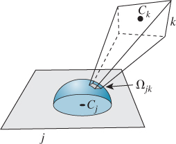
Figure 31.13: Patch k is visible from patch j; when it’s projected onto the hemisphere around Cj, we get a solid angle called ωjk.
Now let’s use these assumptions to simplify the rendering equation. Let’s start with a point P in some patch j. The rendering equation says that for a direction ωo with ωo · nj > 0, that is, an outgoing direction from patch j,
We now introduce some factors of π to simplify the equation a bit. We let Bj = L(P, ωo)/π. Since L(P, ωo) is assumed independent of the outgoing direction ωo, the number Bj does not have ωo as a parameter. Similarly, we define Ej = Le(P, ωo)/π. And substituting fr(P, ωi, ωo) = ρj/π, we get
The inner integral, over all directions in the positive hemisphere, can be broken into a sum over directions in each Ωjk, since light arriving at patch j must arrive from some patch k. The equation thus becomes

The radiance in the integral is radiance leaving patch k, and is therefore just πBk. Substituting, and rearranging the constant factors of π a little, we get
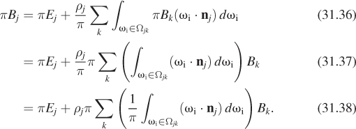
Dividing through by π, we get
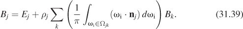
The coefficient of Bk inside the summation is called the form factor fjk for patches j and k. So the equation becomes
which is called the radiosity equation. Before we try to solve it, let’s look at the form factor more carefully. For patches j and k, it is
Using the second assumption (that all rays from patch k to patch j are essentially the same) we see that the vector ωi can be replaced by ujk = S(Ck – Cj), the unit vector pointing from the center of patch j to the center of patch k. Since ujk · nj is a constant, it can be factored out of the integral.
The form factor can then be written:
The remaining integral is just the measure of the solid angle Ωjk, which is the area Ak of patch k, divided by the square of the distance between the patches (i.e., by ||Cj–Ck||2), using the third assumption and scaled down by the cosine of the angle between nk and ujk (by the Tilting principle). Thus, the form factor becomes
(a) The form of Equation 31.44 makes it evident that fjk/Ak = fkj/Aj. Explain why, if j and k are mutually visible, exactly one of the two dot products is negative.
(b) Suppose that patch k is enormous and occupies essentially all of the hemisphere of visible directions from patch j. What will the value of fjk be, approximately?
If we compute all the numbers fjk and assemble them into a matrix, which we multiply by a diagonal matrix D(ρ) whose jth diagonal entry is ρj, and we assemble the radiosity values Bj and emission values Ej into vectors b and e, then the radiosity equation, under the assumptions listed above, becomes
This can be simplified (just like the integral form of the rendering equation) to
which is just a simple system of linear equations (albeit possibly with many unknowns).
Standard techniques from linear algebra can be used to solve this equation (see Exercise 31.2).![]() The existence of a solution depends on the matrix D(ρ)F being “small” compared to the identity, that is, having all eigenvalues less than one. This is a consequence of our assumption that all the reflectivities were less than one (and your computation of the largest possible form factor). Note that we do not suggest solving the equation by inverting the matrix; in general that’s O(n3), while approximation techniques like Gauss-Seidel work extremely well (and much faster) in practice.
The existence of a solution depends on the matrix D(ρ)F being “small” compared to the identity, that is, having all eigenvalues less than one. This is a consequence of our assumption that all the reflectivities were less than one (and your computation of the largest possible form factor). Note that we do not suggest solving the equation by inverting the matrix; in general that’s O(n3), while approximation techniques like Gauss-Seidel work extremely well (and much faster) in practice.
Computing fjk is a once-per-scene operation. Once the matrix F is known, we can vary the lighting conditions (the vector e) and then recompute the emitted radiance at each patch center (the vector b) quite quickly.
Once we know the vector b, how do we create a final image, given a camera specification? We can create a scene consisting of rectangular patches, where patch j has value Bj, and then rasterize the scene from the point of view of the camera. Instead of computing the lighting at each pixel, we use the value stored for the surface shown at that pixel: if that pixel shows patch j, we store the value πBj at that pixel. The resultant radiance image is a radiosity rendering of the scene.
This, however, is rarely done as described; such a radiosity rendering looks very “blocky,” while we know from experience that totally Lambertian environments tend to have very smoothly varying radiance. Instead of rendering the computed radiance values directly, we usually interpolate them between patch centers, using some technique like bilinear interpolation, or even some higher-order interpolation. This is closely analogous to the approach discussed in Section 31.4, in which we solved an equation on the integers and then interpolated to guess a solution on the whole real line. In this case, we’ve found a piecewise-constant function (represented by the vector b) that satisfies our discretized approximation of the rendering equation, but we’re displaying a different function, one that’s not piecewise constant.
![]() What we’ve done is to take the space V of all possible surface radiance fields, and consider only a subset W of it, consisting of those that are piecewise constant on our patches. We’ve approximated the equation and found a solution to this in W; we’ve then transformed this solution (by linear interpolation) into a different subspace D consisting of all piecewise-linear radiance fields. If D and W are “similar enough,” then this is somewhat justified (see Figure 31.14).
What we’ve done is to take the space V of all possible surface radiance fields, and consider only a subset W of it, consisting of those that are piecewise constant on our patches. We’ve approximated the equation and found a solution to this in W; we’ve then transformed this solution (by linear interpolation) into a different subspace D consisting of all piecewise-linear radiance fields. If D and W are “similar enough,” then this is somewhat justified (see Figure 31.14).
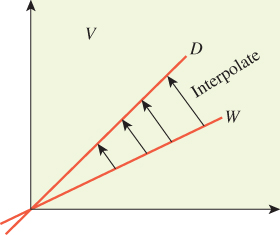
Figure 31.14: Schematically, the space V of all surface-radiance fields contains a subspace W of piecewise constant fields, and another subspace D of piecewise linear fields. There’s a map from W to D defined by linear interpolation.
One way to address this apparent contradiction is to not assume that the radiance is piecewise constant, and instead assume it’s piecewise linear, or piecewise quadratic, and do the corresponding computations. Cohen and Wallace [CWH93] describe this in detail.
The computation of form factors is the messiest part of the radiosity algorithm. One approach is to render the entire scene, with a rasterizing renderer, five times, projecting onto the five faces of a hemicube, (the top half of a cube as shown in Figure 31.15). Rather than storing a radiance value at each pixel, you store the index k of the face visible at that pixel. You can precompute the projected solid angle for each “pixel” of a hemicube face once and for all; to compute the projected solid angle subtended by face k, you simply sum these pixel contributions over all pixels storing index k. For this to be effective, the hemicube images must have high enough resolution that a typical patch projects to hundreds of hemicube “pixels”; as scene complexity grows (or as we reduce the patch size to make the “constant radiance on each patch” assumption more correct), this requires hemicube images with increasingly higher resolution.
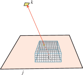
Figure 31.15: We project the scene onto a hemicube around P; since patch k is visible from P through the pixel shown, the hemicube image at that pixel stores the value k.
In solving the radiosity equation, Equation 31.46, some approximation techniques do not use every entry of F; it therefore makes sense to compute entries of F on the fly sometimes, perhaps caching them as you do so. Various approaches to this are described in great detail by Cohen and Wallace [CWH93].
Before we leave the topic of radiosity, we should mention four more things.
First, in our development, we assumed that patches were completely mutually visible; the hemicube approach to computing form factors removes this requirement. On the other hand, the hemicube approach does assume that the solid angle subtended by patch k from the center of patch j is a good representation of the solid angle subtended at any other point of patch j. That’s fine when j and k are distant, but when they’re nearby (e.g., one is a piece of floor and another is a piece of wall, and they share an edge) the assumption is no longer valid. The form-factor computation must then be written out as an integral over all points of the two patches, and even for simple geometries it has, in general, no simple expression. Schroeder [SH93] expresses this form factor in terms of (fairly) standard functions, but the expression is too complex for practical use.
Second, meshing has a large impact on the quality of a radiosity solution; in particular, if there are shadow edges in the scene, the final quality is far better if the mesh edges are aligned with those shadow edges, or if the patches near those edges are very small (so that they can effectively represent the rapid transition in brightness near the edge). Lischinski et al. [LTG92] describe approaches to precomputing meshes that are well adapted to representing the rapid transitions that will appear during a radiosity computation.
A different approach to the meshing problem is to examine, for each patch, the assumption of constant irradiance across the patch. We do this by evaluating the irradiance at the corners of the patch and comparing them. If the difference is great enough, we split the patch into two smaller patches and repeat, thus engaging in progressive refinement. This approach is not guaranteed to work: It’s possible that, for some patch, the irradiance varies wildly across the patch but happens to be the same at all corners; in this case, we should subdivide, but we will not. One thing that’s fortunate about this approach is that when we subdivide, there’s relatively little work to do: We need to compute the form factors for the newly generated subpatches and remove the form factors for the patch that was split. We also need to take the current surface-radiance estimate for the split patch and use it to assign new values to the subpatches; it suffices to simply copy the old value to the subpatches, although cleverer approaches may speed convergence.
Third, although radiosity, as we have described it, treats only pure-Lambertian surfaces and emitters, one can generalize it in many directions: Instead of assuming that outgoing radiance is independent of direction, one can build meshes in both position and direction (i.e., subdivide the outgoing sphere at point Ci into small patches, on each of which the radiance is assumed constant); this allows for more general reflectance functions, but it increases the size of the computation enormously. Alternatively, one can represent the hemispherical variation of the emitted light in some other basis, such as spherical harmonics; an expansion in spherical harmonics is the higher-dimensional analogue of writing a periodic function using a Fourier series. Ramamoorthi et al. [RH01] have used this approach in studying light transport. In each case, specular reflections are difficult to handle: We either need very tiny patches on the sphere’s surface, or we need very high-degree spherical harmonics, both of which lead to an enormous increase in computation. One approach to this problem is to separate out “the specular part” of light transport into a separate pass. Hybrid radiosity/ray-tracing approaches [WCG87] attempt to combine the two methods, but this approach to rendering has largely given way to stochastic approaches in recent years.
Fourth, we’ve been a little unfair to radiosity. The simplification of the rendering equation under the assumption that all emittance and reflectance is Lambertian is the true “radiosity equation.” It’s quite separate from the division of the scene into patches, and the resultant matrix equation. Nonetheless, the two are often discussed together, and the matrix form is often called the radiosity equation. Cohen and Wallace’s first chapter discusses radiosity in full generality, and treats the discretization approach we’ve described as just one of many ways to approximate solutions to the equation.
31.11. Separation of Transport Paths
The distinction between diffuse and specular reflections is so great that it generally makes sense to handle them separately in your program. For instance, if a surface reflects half its light in the mirror direction, absorbs 10%, and scatters the remaining 40% via Lambert’s law, your code for computing an outgoing scattering direction from an incoming direction will look something like that in Listing 31.1. This is the algorithmic version of the discussion in Section 29.6, and it involves the ideas of mixed probabilities discussed in Chapter 30.
Listing 31.1: Scattering from a partially mirrorlike surface.
1 Input: an incoming direction wi, and the surface normal n
2 Output: an outgoing direction wo, or false if the light is absorbed
3
4 function scatter(...):
5 r = uniform(0, 1)
6
7 if (r > 0.5): // this is mirror scattering
8 wo = -wi + 2 * dot(wi, n) * n;
9 else if (r > 0.1): // diffuse scattering
10 wo = sample from cosine-weighted upper hemisphere
11 else: // absorbed
12 return false;
31.12. Series Solution of the Rendering Equation
The rendering equation, written in the form
is an equation of the form
that’s familiar from linear algebra, except that in place of a vector x of three or four elements, we have an unknown function, L; instead of a target vector b, we have a target function, the emitted radiance field Le; and instead of the linear transformation being defined by multiplication by a matrix M, it’s defined by applying some linear operator. ![]() Roughly speaking, the difference is between the finite-dimensional problems familiar from linear algebra, and the infinite-dimensional problems that arise when working with spaces of real-valued functions. (Indeed, the radiosity approximation amounts to a finite-dimensional approximation of the infinite-dimensional problem, so the radiosity equation ends up being an actual matrix equation.)
Roughly speaking, the difference is between the finite-dimensional problems familiar from linear algebra, and the infinite-dimensional problems that arise when working with spaces of real-valued functions. (Indeed, the radiosity approximation amounts to a finite-dimensional approximation of the infinite-dimensional problem, so the radiosity equation ends up being an actual matrix equation.)
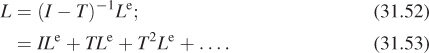
For the moment, let’s pretend that the problem we care about really is finite dimensional: that L is a vector of n elements, for some large n, and so is Le, while I – T is an n × n matrix. The solution to the equation is then
In general, computing the inverse of an n × n matrix is quite expensive and prone to numerical error, particularly for large n. But there’s a useful trick. We observe that
Verify Equation 31.50 by multiplying everything out. Remember that matrix multiplication isn’t generally commutative. Why is it OK to swap the order of multiplications in this case?
Suppose that as k gets large, Tk+1 gets very small (i.e., all entries of Tk+1 approach zero). Then the sum of all powers of T ends up being the inverse of (I – T), that is, in this special case we can in fact write
Multiplying both sides by Le, we get
In words, this says that the light in the scene consists of that emitted from the luminaires (ILe), plus the light emitted from luminaires and scattered once (TLe), plus that emitted from luminaires and scattered twice (T2Le), etc.
Our fanciful reasoning, in which we assumed everything was finite-dimensional, has led us to a very plausible conclusion. In fact, the reasoning is valid even for transformations on infinite-dimensional spaces. The only restriction is that T2 must be interpreted as “apply the operator T twice” rather than “square the matrix T.”
We did have to assume that Tk ![]() 0 as k gets large, however. When T is a matrix, this simply means that all entries of Tk go toward zero as k gets large. For a linear operator on an infinite dimensional space, the corresponding statement is that TkH goes to zero as k gets large, where H is an arbitrary element of the domain of T. (In our case, this means that for any initial emission values, if we trace the light through enough bounces, it gets dimmer and dimmer.)
0 as k gets large, however. When T is a matrix, this simply means that all entries of Tk go toward zero as k gets large. For a linear operator on an infinite dimensional space, the corresponding statement is that TkH goes to zero as k gets large, where H is an arbitrary element of the domain of T. (In our case, this means that for any initial emission values, if we trace the light through enough bounces, it gets dimmer and dimmer.)
We’ll assume, from now on, that the scattering operator T has the property that Tk ![]() 0 as k
0 as k ![]() ∞ so that the series solution of the rendering equation will produce valid results.
∞ so that the series solution of the rendering equation will produce valid results.
Of course, the series solution has infinitely many terms to sum up, each of them expensive to compute, so it’s not, as written, a practical method for rendering a scene. On the other hand, as we’ve already seen with radiosity, there are practical approximations to be made based on this series solution.
![]() When do high powers of a linear operator approach the zero operator? We can answer this by looking at eigenvalues: If all eigenvalues are strictly less than one, then TkLe
When do high powers of a linear operator approach the zero operator? We can answer this by looking at eigenvalues: If all eigenvalues are strictly less than one, then TkLe ![]() 0 as k goes to ∞. In rendering, this more or less corresponds to there being no perfect reflectors in a scene; indeed, one can imagine a scene consisting of two enormous planar mirrors that face each other, and a point light source between them. Equal amounts of light moving left and right constitute an eigenvector of the light-scattering operator T: After reflection, we once again have equal amounts of light moving left and right. So in this situation, T has an eigenvalue of 1, and iterative computation is not guaranteed to converge. Indeed, if the light source puts out some light, a moment later that light will be reflected by the mirrors and will be added to new light sent out by the source, etc., so that the transported light goes to infinity. The unrealistic assumption of perfect mirrors leads to the unrealistic prediction of infinite light transport (and the nonconvergence of the iterative method for solving the equation).
0 as k goes to ∞. In rendering, this more or less corresponds to there being no perfect reflectors in a scene; indeed, one can imagine a scene consisting of two enormous planar mirrors that face each other, and a point light source between them. Equal amounts of light moving left and right constitute an eigenvector of the light-scattering operator T: After reflection, we once again have equal amounts of light moving left and right. So in this situation, T has an eigenvalue of 1, and iterative computation is not guaranteed to converge. Indeed, if the light source puts out some light, a moment later that light will be reflected by the mirrors and will be added to new light sent out by the source, etc., so that the transported light goes to infinity. The unrealistic assumption of perfect mirrors leads to the unrealistic prediction of infinite light transport (and the nonconvergence of the iterative method for solving the equation).
In practice, most surfaces we encounter have relatively low reflectance, and an iterative computation not only converges, it converges fairly quickly. Unfortunately, the convergence isn’t necessarily the kind we want: Our estimate of the radiance field L, after a few iterations, may be very close to the true radiance field L0, but the scene’s appearance to a human observer might be very different. For instance, if the scene consists of a room lit by a tiny pinhole, behind which there’s a light source, the true light in the room is very small ... and therefore very similar to no light in the room; similar, that is, when we compare using the standard mathematical measure of similarity. When we compare using a perceptual metric, the difference is clear: A tiny bit of light when you awaken at night lets you avoid stubbing your toe, while no light at all does not!
31.13. Alternative Formulations of Light Transport
We’ve described light transport in term of the radiance field, L, which is defined on R3 × S2 or ![]() × S2, where
× S2, where ![]() is the set of all surface points in a scene. (Since radiance is constant along rays in empty space, knowing L at points of
is the set of all surface points in a scene. (Since radiance is constant along rays in empty space, knowing L at points of ![]() determines its values on all of R3.) And we’ve used the scattering operator, which transforms an incoming radiance field to an outgoing one in writing the rendering equation. But there are alternative formulations.
determines its values on all of R3.) And we’ve used the scattering operator, which transforms an incoming radiance field to an outgoing one in writing the rendering equation. But there are alternative formulations.
Arvo [Arv95] describes light transport in terms of two separate operators. The first operator, G, takes the surface radiance on ![]() and converts it to the field radiance, essentially by ray casting: Surface radiance leaving a point P in a direction ω becomes field radiance at the point Q where the ray first hits
and converts it to the field radiance, essentially by ray casting: Surface radiance leaving a point P in a direction ω becomes field radiance at the point Q where the ray first hits ![]() . The second operator, K, takes field radiance at a point P and combines it with the BRDF at P to produce surface radiance (i.e., it describes single-bounce scattering locally). Thus, the transport operator T can be expressed as T = K ο G.
. The second operator, K, takes field radiance at a point P and combines it with the BRDF at P to produce surface radiance (i.e., it describes single-bounce scattering locally). Thus, the transport operator T can be expressed as T = K ο G.
Kajiya [Kaj86] takes a different approach in which light directly transported from any point P ![]() M to any point Q
M to any point Q ![]() M is represented by a value I(P, Q); if P and Q are not mutually visible, then I(P, Q) is zero. Kajiya calls the quantity I the unoccluded two-point transport intensity. (The letters I, ρ, M, and g used in this and the following section will not be used again; we are merely explaining the correspondence between his notation and ours.) Kajiya’s version of the BRDF is not expressed in terms of a point and two directions, but rather in terms of three points; he writes ρ(P, Q, R) for the amount of light from R to Q that’s scattered toward the point P. His “emitted light” function also has points as parameters rather than point-direction parameters:
M is represented by a value I(P, Q); if P and Q are not mutually visible, then I(P, Q) is zero. Kajiya calls the quantity I the unoccluded two-point transport intensity. (The letters I, ρ, M, and g used in this and the following section will not be used again; we are merely explaining the correspondence between his notation and ours.) Kajiya’s version of the BRDF is not expressed in terms of a point and two directions, but rather in terms of three points; he writes ρ(P, Q, R) for the amount of light from R to Q that’s scattered toward the point P. His “emitted light” function also has points as parameters rather than point-direction parameters: ![]() (P, Q) is the amount of light emitted from Q in the direction of P. Kajiya’s quantities exclude various cosines that appear in our formulation of the rendering equation, including them instead as part of the integration (his integrals are over the set
(P, Q) is the amount of light emitted from Q in the direction of P. Kajiya’s quantities exclude various cosines that appear in our formulation of the rendering equation, including them instead as part of the integration (his integrals are over the set ![]() of all surfaces in the scene, while ours are usually over hemispheres around a point; the change-of-variables formula introduces the necessary cosines, as described in Section 26.6.4). Kajiya’s formulation of the rendering equation is therefore
of all surfaces in the scene, while ours are usually over hemispheres around a point; the change-of-variables formula introduces the necessary cosines, as described in Section 26.6.4). Kajiya’s formulation of the rendering equation is therefore
where g(P, Q) is a “geometry” term that in part determines the mutual visibility of P and Q: It’s zero if P is occluded from Q. Expressing this in terms of operators, he writes
where M is the operator that combines I with ρ in the integral. The series solution then becomes
This formulation has the advantage that the computation of visibility is explicit: Every occurrence of g represents a visibility (or ray-casting) operation.
31.14. Approximations of the Series Solution
As we mentioned, summing an infinite series to solve the rendering equation is not really practical. But several approximate approaches have worked well in practice. We follow Kajiya’s discussion closely.
The earliest widely used approximate solution consisted (roughly) of the following:
• Limiting the emission function to point lights
• Computing only one-bounce scattering (i.e., paths of the form LDE)
That is to say, the approximation to Equation 31.56 used was
where ![]() 0 denotes the use of only point lights. (The first term has
0 denotes the use of only point lights. (The first term has ![]() , because it was possible to render directly visible area lights.) Note that the second term should have been gMg
, because it was possible to render directly visible area lights.) Note that the second term should have been gMg![]() 0, that is, it should have accounted for whether the illumination could be seen by the surface (i.e., was the surface illuminated?). But such visibility computations were too expensive for the hardware, with the result that these early pictures lacked shadows.
0, that is, it should have accounted for whether the illumination could be seen by the surface (i.e., was the surface illuminated?). But such visibility computations were too expensive for the hardware, with the result that these early pictures lacked shadows.
Note that since ![]() 0 consisted of a finite collection of point lights, the integral that defines M became a simple sum.
0 consisted of a finite collection of point lights, the integral that defines M became a simple sum.
As an approach to solving the rendering equation, this involves many of the methods described in Section 31.2: The restriction to a few point lights amounts to solving a subproblem. The truncation of the series amounts to approximating the solution method rather than the equation. The transport operator, M, used in the early days was also restricted: All surfaces were Lambertian, although this was soon extended to include specular reflections as well.
Improving the algorithm to use g![]() 0 instead of
0 instead of ![]() 0 (i.e., including shadows) was a subject of considerable research effort, with two main approaches: exact visibility computations, and inexact ones. Exact visibility computations are discussed in Chapter 36.
0 (i.e., including shadows) was a subject of considerable research effort, with two main approaches: exact visibility computations, and inexact ones. Exact visibility computations are discussed in Chapter 36.
A typical inexact approach consists of rendering a scene from the point of view of the light source to produce a shadow map: Each pixel of the shadow map stores the distance to the surface point closest to the light along a ray from the light to the surface. Later, when we want to check whether a point P is illuminated by the light, we project P onto the shadow map from the light source, and check whether it is farther from the light source than the distance value stored in the map. If so, it’s occluded by the nearer surface and hence not illuminated. This approach has many drawbacks, the main one being that a single sample at the center of a shadow map pixel is used to determine the shadow status of all points that project to that pixel; when the view direction and lighting direction are approximately opposite, and the surface normal is nearly perpendicular to both, this can lead to bad aliasing artifacts (see Figure 31.16).
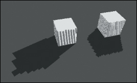
Figure 31.16: Aliasing produced by a low-resolution shadow map. The aliasing on the shadows is the problem; the stripes on the cubes themselves arise from a different problem. (Courtesy of Fabien Sanglard.)
By the way, the approaches used in the early days of graphics were not, at the time, seen as approximate solutions to the rendering equation. They were practical “hacks,” sometimes in the form of applications of specific observations (e.g., Lambert’s law for reflection from a diffuse surface) to more general situations than appropriate, and sometimes were approximations to the phenomena that were observed, without any particular reference to the underlying physics. When you read older papers, you’ll seldom see units like watts or meters; you’ll also on rare occasions notice an extra cosine or a missing one. Be prepared to read carefully and think hard, and trust your own understanding.
31.15. Approximating Scattering: Spherical Harmonics
We’ve discussed patch-based radiosity, in which the field radiance is approximated by a piecewise constant function; one can also think of this as an attempt to write the field radiance in a particular basis for a subspace of all possible field-radiance functions, in this case the basis consisting of functions that are identically one on some patch j, and zero everywhere else. Linear combinations of these functions are the piecewise constant functions used in radiosity.
A similar approach is to represent the surface radiance at a point (which is a function on the hemisphere of incoming directions) in some basis for the space of functions on the sphere. Assuming we limit ourselves to continuous functions, such a basis is provided by spherical harmonics, h1, h2, ..., which are the analog, for S2, of the Fourier basis functions sin(2πnx) (n = 1, 2, ...) and cos(2πnx) (n = 0, 1, 2, ...) on the unit circle. The first few spherical harmonics, in xyz-coordinates, are proportional to 1, x, y, z, xy, yz, zx, and x2 – y2, with the constant of proportionality chosen so that each integrates to one on the sphere. In spherical polar coordinates, they can be written 1, cos θ, sin θ, sin φ, sin 2θ, sin θ sin φ, cos θ cos φ, and cos 2θ. Like the Fourier basis functions on the circle, they are pairwise orthogonal: The integral of the product of any two distinct harmonics over the sphere is zero. Figure 31.17 shows the first few harmonics, plotted radially. The plot of h1, which is the constant function 1, yields the unit sphere.
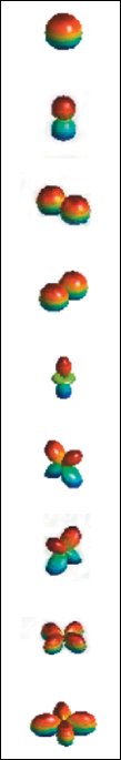
Figure 31.17: The first few spherical harmonics. For each point on the unit sphere (1, θ, φ) in spherical polar coordinates, we plot a point (r, θ, φ), where r = | hj(θ, φ)|. The absolute value avoids problems where negative values get hidden, but is slightly misleading.
To be clear: If you have a continuous function f : S2 ![]() R, you can write f as a sum3 of spherical harmonics:
R, you can write f as a sum3 of spherical harmonics:
3. ![]() Limiting to a finite sum gives an approximation to the function; if f is discontinuous, then the sum converges to f only in regions of continuity.
Limiting to a finite sum gives an approximation to the function; if f is discontinuous, then the sum converges to f only in regions of continuity.
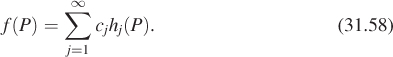
The coefficients cj depend on f, of course, just as when we wrote a function on the unit circle as a sum of sines and cosines, the coefficients of the sines and cosines depended on the function. In fact, they’re determined the same way: by computing integrals.
The cosine-weighted BRDF at a fixed point P is a function of two directions ωi and ωo, that is, the expression
defines a map ![]() . So the preceding statement about representing functions on S2 via harmonics does not directly apply. But we can approximate the cosine-weighted BRDF
. So the preceding statement about representing functions on S2 via harmonics does not directly apply. But we can approximate the cosine-weighted BRDF ![]() at P with spherical harmonics in a two-step process. To simplify notation, we’ll omit the argument P for the remainder of this discussion.
at P with spherical harmonics in a two-step process. To simplify notation, we’ll omit the argument P for the remainder of this discussion.
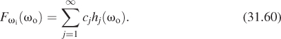
First, we fix ωi and consider the function ωo ![]()
![]() (ωi, ωo); this function on S2—let’s call it Fωi—can be expressed in spherical harmonics:
(ωi, ωo); this function on S2—let’s call it Fωi—can be expressed in spherical harmonics:
If we chose a different ωi, we could repeat the process; this would get us a different collection of coefficients {cj}. We thus see that the coefficients cj depend on ωi; we can think of these as functions of ωi and write
Now each function ωi ![]() cj(ωi) is itself a function on the sphere, and can be written as a sum of spherical harmonics. We write
cj(ωi) is itself a function on the sphere, and can be written as a sum of spherical harmonics. We write
Substituting this expression into Equation 31.61, we get
The advantage of this form of the expression is that when we evaluate the integral at the center of the rendering equation, namely,
both L and fs are expressed in the spherical harmonic basis. This will soon let us evaluate the integral very efficiently. Note, however, that in expressing the BRDF as a sum of harmonics, we were assuming that the BRDF was continuous; this either rules out any impulses (like mirror reflection), or requires that we replace all equalities above by approximate equalities.
Unfortunately, while L may be expressed with respect to the global coordinate system, fs is usually expressed in a coordinate system whose x- and z-directions lie in the surface, and whose y-direction is the normal vector. Transforming L’s spherical-harmonic expansion into this local coordinate system requires some computation; it’s fairly straightforward for low-degree harmonics, but it gets progressively more expensive for higher degrees. If we write the field radiance L at point P in spherical harmonics in this local coordinate system (absorbing a minus sign as we do so),
then the central integral takes the form
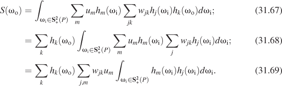
The integral in this expression is 0 if j and m differ, and 1 if they’re the same. So the entire expression simplifies to express the surface radiance in direction ωo as
The inner sum can be seen as a matrix product between the row vector u of the coefficients of the field radiance and the matrix of coefficients for the cosine-weighted BRDF. The product vector provides the coefficients for the surface radiance in terms of spherical harmonics in the local coordinate system.
At the cost of expressing the BRDF and field radiance in terms of spherical harmonics, we’ve converted the central integral into a matrix multiplication. This is another instance of the Basis principle: Things are often simpler if you choose a good basis. In particular, if you’re likely to be integrating products, a basis like the spherical harmonics, in which the basis functions are pairwise orthogonal, is especially useful.
If the field radiance can be assumed to be independent of position (e.g., if most light comes from a partly overcast sky), then the major cost in this approach is transforming the spherical harmonic expression for field radiance in global coordinates to local coordinates. If not, there’s the further problem of converting surface radiance at one point, expressed in terms of spherical harmonics there, into field radiance at other points, expressed in terms of spherical harmonics at those points.
This approach, which we’ve only sketched here, has been developed thoroughly by Ramamoorthi [RH01]. There are several important challenges.
• There is a conversion of harmonic decompositions in different coordinate systems, which we’ve already described.
• We replaced the work of integration with the work of matrix multiplication; that’s only a good idea if the matrix size is not too large. Unfortunately, the more “spiky” a function is, the more terms you need in its spherical-harmonic series to approximate it well (just as we need high-frequency sines and cosines to approximate rapidly changing functions in one dimension). Since many BRDFs are indeed spiky (mirror reflectance is a particularly difficult case), a good approximation may require a great many terms, making the matrix multiplication expensive, especially if the matrix is not sparse.
• We’ve ignored a critical property of irradiance at surfaces: It’s nonzero only on the upper hemisphere. That makes the equator generally a line of discontinuity, and fitting spherical harmonics to discontinuities is difficult: A good fit requires more terms.
Ramamoorthi makes a strong argument for much of field radiance being well represented by just the first few spherical harmonics. Sloan [Slo08] has written a useful summary of properties of spherical harmonics, and with Kautz and Snyder [KSS02] has shown how to use them very efficiently in rendering scenes with either fixed view and moving lights, or vice versa.
31.16. Introduction to Monte Carlo Approaches
We now move on to Monte Carlo techniques for solving the rendering equation. The basic idea is to estimate the integral in the rendering equation (or some other integral) by probabilistic methods, which we discussed in Chapter 29. Broadly speaking, we collect samples of the integrand and average them, multiplying the size of the domain of integration.
We begin with a broad and informal view of the various techniques we’ll be examining.
Classic ray tracing, which you already saw in Chapter 15, consists of repeatedly casting a ray from the eye and determining the color of the point where it first intersects a surface in the scene. This color is the sum of the illumination from each visible light source (we use ray casting to check visibility), plus illumination from elsewhere in the scene, which we only compute if the intersection point has some specular component, in which case we recursively trace the reflected or refracted ray.
In Chapter 15, we only computed the direct illumination, but modifying a ray tracer to include the recursive part is fairly straightforward. Listing 31.2 gives the pseudocode for point light sources.
The use of “color” here is a shorthand for “spectral radiance distribution,” but the main idea is that there’s some quantity we can compute by evaluating direct illumination at the intersection point, and a remaining quantity that we compute by a recursion. We must generally cast rays from the eye through every pixel in the image we’re computing, and we often use multiple samples per pixel, with some kind of averaging. But the broad idea remains: Cast rays from the eye; compute direct illumination; add in recursive rays. Ray tracing computes the contributions of paths of the form LD?S*E.
Listing 31.2: Recursive ray tracing.
1 foreach pixel (x, y):
2 R = ray from eyepoint E through pixel
3 image[x, y] = raytrace(R)
4
5 raytrace(R):
6 P = raycast(R) // first scene intersection
7 return lightFrom(P, R) // light leaving P in direction opposite R
8
9 lightFrom(P, R):
10 color = emitted light from P in direction opposite R.
11 foreach light source S:
12 if S is visible from P:
13 contribution = light from S scattered at
14 P in direction opposite R
15 color += contribution
16 if scattering at P is specular:
17 Rnew = reflected or refracted ray at P
18 color += raytrace(Rnew)
19 return color
The essential features of a ray tracer (and all the subsequent algorithms) are a ray-casting function (something that lets us shoot a ray into a scene and find the first surface it encounters), and a BRDF or bidirectional scattering distribution function (BSDF), which takes a surface point P and two rays ωi and ωo and returns fs(P, ωi, ωo). (In the pseudocode, that BRDF is hidden in the “light from S scattered at P in direction opposite R,” which has to be computed by multiplying the radiance from the light by a cosine and the BRDF to get the scattered radiance.) A slightly more sophisticated ray tracer removes the “if scattering is specular” condition, and if the scattering is nonspecular, the scattered radiance is estimated by casting multiple recursive rays in many directions, weighting the returned results by the BSDF according to the reflectance equation. It’s this form of ray tracing that we’ll refer to henceforth.
Later, in addition to the BRDF or BSDF, we’ll also want a function that takes a surface point P and a ray ωi and returns a random ray ωo with probability density approximately proportional to the BRDF or BSDF, or cosine-weighted versions of these.
Following Kajiya, we can draw a highly schematic representation of ray tracing (see Figure 31.18). Rays are traced from the eye to the scene; at an intersection, we compute direct lighting and accumulate it as part of the radiance from the light to the eye along the leftmost segment of the path. We also cast recursive rays. In basic ray tracing, we only do so in the specular-bounce direction (if the surface is partly specular); in more sophisticated approaches, we may do so in many directions. When a recursive ray meets a different surface point, the direct lighting there is propagated back to the first intersection, and thence to the eye. This propagation involves two scattering operations. Further depths involve further scattering. In the end, we have a branching tree representing the gathering of light into a single pixel of the final image. The branching factor of the tree depends on the number of recursively cast rays at each scattering event.
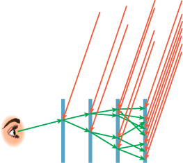
Figure 31.18: Each blue vertical line represents all of ![]() , the set of points of the scene; a green path from the eye (at left) meets
, the set of points of the scene; a green path from the eye (at left) meets ![]() at some point, and then recursively, multiple rays are traced; these meet the second copy of
at some point, and then recursively, multiple rays are traced; these meet the second copy of ![]() , etc. Each branching at such an intersection is a scattering event. The red rays from the upper right to the ray-surface intersections represent light arriving from light sources, which in this schematic representation are placed infinitely far away so that all direct illuminations can be drawn parallel.
, etc. Each branching at such an intersection is a scattering event. The red rays from the upper right to the ray-surface intersections represent light arriving from light sources, which in this schematic representation are placed infinitely far away so that all direct illuminations can be drawn parallel.
In path tracing, rays are again cast from the eye, and direct illumination is again computed, but a single recursive ray is also cast, not necessarily in the specular direction: The direction for the recursive ray is determined by some probability distribution on possible directions. The result is to effectively compute the contributions of all paths of the form L(S|D) * E. Because of the probabilistic nature of the algorithm, we get noise in the resultant image. To reduce the noise, a great many rays must be cast. The schematic representation (see Figure 31.19) of path tracing is similar to that for ray tracing, except that the branching factor for each tree is one. There are, however, many more trees associated to each pixel (although we only draw one).
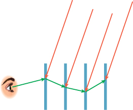
Figure 31.19: In path tracing, each path from the eye either terminates with some probability or traces a single recursive ray. In the version of the algorithm schematically depicted here, direct-light contributions to light transport along the path are computed at every scattering or absorption point, and then transported back along the path.
In bidirectional path tracing, one path is traced from the eye and another path is traced from a light source. By splicing together these paths (say, the third point on the light path gets joined to the second point on the eye path), we create paths that may carry light all the way from the source to the eye. If the splice segment meets an occluder, we get no light transport at all, however. Each spliced path gives information about light going to the eye (or camera), and we take the information from multiple paths and splicings to estimate the color of each pixel. Bidirectional path tracing drastically improves the handling of caustics (bright regions arising from paths of the form LS+DE, i.e., light focused in various ways on a diffuse surface). When caustics are seen only in reflection (e.g., with paths of the form LS+DSE), or when they arise not directly from a light source, but from its reflection in a small diffuse object (LDS+DE), they are once again difficult to compute, however.
The schematic representation of bidirectional path tracing (see Figure 31.20) consists of two trees, one starting from a light and one starting from the eye, with splices between all pairs of interior nodes. Again, we have to understand that there are many paths for each image pixel and many paths emanating from each light source, so a more accurate schematic would consist of two forests with many possible splices.
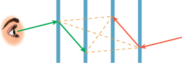
Figure 31.20: In bidirectional path tracing, we compute many eye paths (green) and many light paths (red), and then consider all possible “splices” (orange) between the two sets.

Figure 31.21: In photon mapping, the forest of light paths is used to estimate the incident light at every surface point by a kind of local interpolation. Eye paths then get incoming radiance values from this estimate, which we draw as a cloud around the leaves of the light-path trees.
One last algorithm we’ll discuss—Metropolis light transport—doesn’t directly fit into this schematization. It does involve bidirectional path tracing, but the paths are chosen and used in a rather different way.
As described informally above, we’ll be recursively tracing lots of rays, forming paths in a scene. In Monte Carlo methods, these paths are generated through a randomized process, usually by sampling from some distribution related to the BRDF.
The two main forms of sampling we tend to do are very similar.
• In ray tracing, we take a ray from the eye to a point P on some surface, and ask, “Which rays arriving at P contribute light that will reach the eye?” For a mirror surface, the answer is “the mirror direction”; for a diffuse surface, it’s “light coming from any direction could produce light in the eye-ray direction.” For others, the answer lies somewhere in between. We need, given the direction ωo, to be able to draw samples from ![]() in a way that’s proportional to ωi
in a way that’s proportional to ωi ![]() fs(ωi, ωo) (perhaps multiplied by a cosine factor).
fs(ωi, ωo) (perhaps multiplied by a cosine factor).
• In methods like photon mapping, where we “push” light out from sources rather than “gathering it toward the eye,” we instead need to address the problem: “Given that some light arrived at this surface point P from direction ωi, it will be scattered in many directions. Randomly provide me an outgoing direction ωo where the probability of selecting ωo is proportional to fs(ωi, ωo).”
Clearly these two problems are closely related.
The collecting of samples is done with a sampling strategy. What we’ve outlined above—“Give me a sample that’s proportional to something”—comes up both in the Metropolis algorithm and in importance sampling. Other sampling strategies can be used in other approaches to integration. Sometimes it’s important to be certain that you’ve got samples over a whole domain, rather than accidentally having them all cluster in one area; in such cases, stratified sampling, Poisson disk sampling, and other strategies can generate good results without introducing harmful artifacts.
Regardless of the sampling approach that we use, the values we compute are always random variables, and their properties, as estimators of the corresponding integrals, are how we can measure the performance of the various algorithms.
Before we proceed, here’s a brief review of what we learned about Monte Carlo integration (following Kellerman and Szirmay-Kalos [KSKAC02]).
To compute the integral of a function f over some domain H, we represent it as an expected value of a random variable:
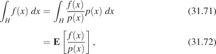
where p is a probability density on the domain H. To estimate the expected value, we draw N mutually uncorrelated samples according to p and average them, resulting in
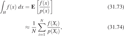
where the standard deviation of this approximation is ![]() , σ2 being the variance of the random variable f(X)/p(X). By choosing p to be large where f is large and small where f is small, we reduce this variance. This is called importance sampling, with p being the importance function. (If the samples are correlated, the variance reduction is not nearly as rapid; we’ll return to this later.)
, σ2 being the variance of the random variable f(X)/p(X). By choosing p to be large where f is large and small where f is small, we reduce this variance. This is called importance sampling, with p being the importance function. (If the samples are correlated, the variance reduction is not nearly as rapid; we’ll return to this later.)
With this in mind, let’s begin with a general approach to approximating the series solution to the rendering equation.
31.17. Tracing Paths
In solving L = Le + TL for the unknown L, we found that the solution could be written
where Le represented the emitted radiance from luminaires, T represented the transport operator, and L was the total radiance in the scene.
Let’s look at ray tracing in this framework: We take a single ray that enters the eye and find the surface point it hits; we then compute direct lighting at that point, and recursively trace more rays, which hit more surface points, where we again compute direct lighting, etc. We are, at the level of computation, building a branching structure: If we trace, on average, n recursive rays at each scattering, then after k steps of scattering, we are tracing nk rays. If the average reflectance is ρ < 1, then the direct lighting at the start of each such ray sequence suffers about ρk attenuation by the time it contributes to the light reaching the eye. For large n, this attenuation is substantial, which means that we’re doing lots of work (O(nk)) to gather up illumination that amounts to a tiny (ρk) fraction of the final result.
Kajiya observed that in many scenes most of the light reaching the eye undergoes at most a few scattering events, and proposed a modified approach, called path tracing, shown schematically in Figure 31.19 as described earlier.
In path tracing, the indirect illumination at a point P is estimated not with n samples, but with a single sample! In this approach, the work done grows linearly with k, the depth of recursive ray tracing. Of course, it’s possible that the single sample misses something important; to resolve this, one can repeatedly trace the same ray from the eye: Each time it arrives at the first scattering event, the recursive sampler will probably choose a different recursive ray. (Indeed, in practice it makes more sense to gather many samples over the area associated to a single pixel in the image [CPC84], so the recursive rays will almost certainly be different.) With the drastically reduced number of recursively traced rays compared to direct ray tracing, we can afford to instead spend this time tracing multiple rays from the eye for each pixel. On average, only a small fraction of the computation time spent on paths of length 1 (directional lighting) is spent on paths of length 2, etc.; this means that only a small amount of effort is expended in estimating the relatively small contribution of indirect illumination.
So far we’ve said nothing about how the path lengths are chosen. In the usual ray-tracing model—pick some recursive depth k and apply recursive ray tracing through k bounces—we will never get contributions from any paths of length more than k, and we will always underestimate the radiance. Hence ray tracing is biased and inconsistent: Even if we trace many rays per pixel, the more-than-k-bounces radiance will never get counted. Path tracing removes the restriction on path length, and thus the corresponding source of bias and inconsistency.
There are two algorithmic drawbacks to path tracing, however. First, the algorithm trades increased accuracy of the mean against increased variance. Having an estimator that can get you the right answer is a great thing, but if you have a small computational budget, then producing an image that’s wrong, but more aesthetically pleasing, may be preferable to producing one that is, on average, correct, but looks very noisy. Second, to reduce bias and move toward a consistent estimator of the final image, the algorithm suffers an unbounded worst-case runtime, although in practice this is rarely a significant problem. The linear-versus-exponential arguments we made earlier don’t tell the whole story. The key idea that Kajiya (and Cook et al.) put forth is that while the time to trace any given ray is about the same, the amount of information that you get from some rays is greater than for others, and you’d like to favor those. If you measure the difference from the true mean of a pixel in a path-traced image that used r rays (total, not just primary rays) and an image produced using r rays in the exponential fan-out pattern, you’ll find that the path-traced image is usually closer to the true mean, that is, the bias is smaller. Kajiya actually leverages the variable importance of rays in several ways; here we’ll just focus on the strategy of sending one (terminal) direct illumination ray and one (recursive) indirect illumination ray at each surface.
31.18. Path Tracing and Markov Chains
We indicated earlier that computing the series solution
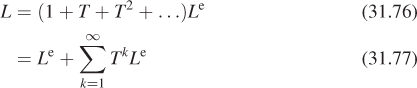
to the rendering equation
where Le is the emitted radiance, L is the radiance, and T is the transport operator, was closely related to computing
as the solution to the equation
where b and x are n-vectors and M is an n × n matrix. The analogy is that T is a linear operator on the space of all possible radiance functions, while multiplication by M is a linear operation on the vector space Rn; in the case where we approximated the space of possible radiance functions by those that are piecewise constant on a fixed mesh, and where the transport operation involved only Lambertian reflection (the radiosity approximation), the analogy was exact: Instead of solving an integral equation, we had to solve a finite-dimensional matrix equation.
We’ll consider the case where M is a 2 × 2 matrix, chosen so that its eigenvalues are both less than one in magnitude, which makes the series converge, and so that its entries are all non-negative, because they’re meant to correspond, roughly, to values of the BSDF in the rendering equation, and these values are never negative.
In the next several pages we’ll estimate the value of x1, the first entry of the solution. We can, of course, solve Equation 31.80 directly, given any particular 2 × 2 matrix M, but you should imagine that M could have a thousand or a trillion rows rather than just two; it’s in that case that the methods described here work best.
We’re going to describe two approaches to finding x1: one nonrecursive and the other recursive. The first is somewhat more complex, and you can skip it if you’d like. The reasons for including it are as follows.
• It provides the justification for the second method.
• The particular formulation is one that you will see often in modern rendering research papers.
31.18.1. The Markov Chain Approach
If we attempt to find the value of x1 using Equation 31.79, we’ll need to sum up infinitely many terms. The first few are
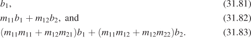
The last term, expanded out, is
From Section 31.5.1, we have a method for estimating such an infinite sum: Select a random term ai in the series (according to some probability distribution p on the positive integers); then ai/p(i) is an estimator for the sum. In this application, we’ll treat each individual summand in Equations 31.81–31.83 as a term, so the first term is b1, the second is m11b1, and so on.
If you look at the sequence of subscripts in any term—say, m12m21b1—you’ll notice the following.
• The subscripts start at 1, because we’re computing the first entry of the answer, x1.
• Each subsequent subscript is repeated twice (in this case, two more twos, then two more ones). This repetition is a consequence of the definition of matrix multiplication.
• Every such sequence occurs.
Thus, to pick a term at random, we need only to pick a “random” finite sequence of subscripts starting at 1. We’ll do so by a slightly indirect method.
Figure 31.22 shows a probabilistic finite-state automaton (FSA). The edge from node i to node j is labeled with a probability pij, which you can read as the probability that if we’re at node i at some moment, we’ll next move to node j. (In a probabilistic FSA of this sort, the path you take through the FSA is not determined by an input string, but instead by random choices at each node.)
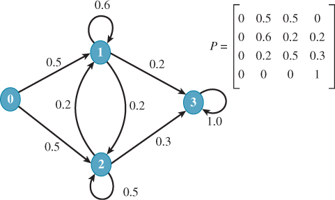
Figure 31.22: A probabilistic FSA with four states, 0, 1, 2, and 3; 0 is the start state; 3 is an absorbing state, and for the remaining states, we have all possible transitions, labeled with probabilities. A graph like this describes a Markov chain. The transition matrix is shown as well.
By starting at node 0 and making random transitions to other states, using the probabilities pij that label the edges of the graph, we’ll eventually arrive at state 3, where we’ll stop. The sequence we generate will start at 0 and end at 3. In between will be a sequence of 1s and 2s that we’ll use as our index sequence.
An FSA like this is a visual representation of a Markov chain—a sequence of states with transition probabilities, with the constraint that the probability of being at some state i at step k + 1 depends only on where you were at step k, and not on any history of your prior steps. Such a Markov chain can be completely described by the matrix P of transition probabilities pij, which has the Markov property: Every row sums to 1 (because when you’re in state i, you have to transition to some state j).
If P is an n × n matrix with the Markov property just described, show that the column vector [1 ... 1]T is a right eigenvector of P. What’s its eigenvalue?
A typical path from state 0 to state 3 in the FSA looks like 01223; the numbers between the first and last states constitute a subscript sequence that corresponds to a term in our summation. In this example, the term is
Furthermore, such a path has a probability of arising from a random walk in the FSA: We write the product of the probabilities for the edges we traveled. In our example, this is
We can now describe a general algorithm for computing the sum in Equation 31.79 (see Listing 31.3).
Listing 31.3: Estimating matrix entries with a Markov chain.
1 Input: A 2 × 2 matrix M and a vector b, both with
2 indices 1 and 2, and the number N of samples to use.
3 Output: an estimate of the solution x to x = Mx + b.
4
5 P = 4 × 4 array of transition probabilities, with indices
6 0,...,3, as in Figure 31.22.
7
8 S1 = S2 = 0 // sums of samples for the two entries of x.
9 repeat N times:
10 s = a path in the FSA from state 0 to state 3, so s(0) = 0.
11 k = length(s) - 2.
12 p = probability for s // product of edge probabilities
13 T = term associated to subscript sequence s(1), s(2),...,s(k)
14 Ss(1) += T/p; // increment the entry of S named by s(1)
15
16 return (S1/N, S2/N)
Under very weak hypotheses on the matrix P, this algorithm provides a consistent estimator of x. That is to say, as N ![]() ∞, the values of S1/N and S2/N will converge to the values of x1 and x2. How fast will they converge? That depends on the matrix P: For some choices of P, the estimator will have low variance, even for small N; for others, it will have large variance. You, as the user of this estimator, get to choose P.
∞, the values of S1/N and S2/N will converge to the values of x1 and x2. How fast will they converge? That depends on the matrix P: For some choices of P, the estimator will have low variance, even for small N; for others, it will have large variance. You, as the user of this estimator, get to choose P.
The following exercises give you a chance to think about “designing” P effectively. While they may seem far removed from rendering, the ideas you get from these exercises will help you understand the approaches taken in path tracing, which we’ll discuss next.
(a) Suppose you know that m12 = 0, and you’re choosing the matrix P in hopes of getting rapid convergence (i.e., low variance in the estimator) of the answer. Is there a reason for picking p12 = 0? Is there a reason for picking p12 ≠ 0? Experiment with ![]() .
.
(b) The transitions represented by p01 and p02 tell us how often (i.e., what fraction of the time) we’re getting a new estimate of x1 and how often we’re getting a new estimate of x2. What are reasonable values for these, and why? How would you choose them if you wanted to only estimate x1?
Write a program to compute the vector x as in Inline Exercise 31.7, and experiment with different transition matrices P to see how they affect convergence. Hint: Experiment with the case where M is a diagonal matrix to see whether you can notice any patterns, and be sure to use only matrices M whose entries are non-negative and whose eigenvalues have magnitudes less than one. (For complex eigenvalues a + bi, this means a2 + b2 < 1.)
We advise that you spend the time doing the inline exercise above, preferably in some language like Matlab or Octave, where such programs are easy to write. Merely debugging your program will give you insight into the method we’ve described.
The “weak conditions” mentioned above are these: First, if mij > 0, then pij > 0. Second, if bi ≠ 0, then pi3 > 0. Together these ensure that any nonzero term in our infinite sum ends up being selected with nonzero probability. The dual of these conditions is also relevant: If bi = 0, then pi3 should be set to zero as well so that we never end up working with a term whose last factor is zero. Similarly, if mij = 0, we save ourselves some work by picking pij = 0.
The corresponding ideas, when we apply what we’ve learned to study light transport, are that (1) we must never ignore any light source (the condition on bi and pi3) and (2) we never want to select a ray direction for which the BSDF is zero, if we can avoid it (the condition on pij being zero).
31.18.1.1. An Alternative Markov Chain Estimator
When we generated the sequence 01223, we used it to compute a single term of the series, and the associated probability. But there’s a slightly different approach, due to Wasow, in which we can use a k-term sequence to generate k different estimates for the sum all at once. It’s described in detail, and a rigorous proof of its correctness is given, in Spanier and Gelbard [SG69]. Here we’ll give an informal derivation of the method.
The idea is this: When we had generated the partial sequence 012, there were several possibilities. We could have generated a 3 next, ending the sequence, or we could have gone on to generate another 1 or 2. If you imagine walking through the FSA thousands of times, some fraction of those times your initial sequence will be 012. If there are 100 such initial sequences, then about 30 of them will be 0123, because p23 = 0.3 in our particular FSA. About 20 of them will have the form 0121 ..., and about 50 will have the form 0122 .... Under the basic scheme, the 30 terminating sequences (0123) would each have associated probability 0.5 · 0.2·0.3 = (0.5·0.20)·0.3, where we’ve put parentheses around everything except the last factor. The associated term in the sum we’re estimating is m12b2, and for each of those 30 sequences, our estimate of the sum is
So, among all sequences starting with 012, 30% contribute ![]() as their estimate of the sum. Suppose that instead we made 100% of the sequences contribute the smaller value
as their estimate of the sum. Suppose that instead we made 100% of the sequences contribute the smaller value ![]() (the division by 0.3 has been removed) as part of their estimate of the sum. The expected value would be the same, because we’d be averaging either 30 copies of the larger value or 100 copies of the smaller value! Of course, we apply the same logic to every single initial sequence, and we arrive at a new version of the algorithm. Before we do so, however, let’s look at the value
(the division by 0.3 has been removed) as part of their estimate of the sum. The expected value would be the same, because we’d be averaging either 30 copies of the larger value or 100 copies of the smaller value! Of course, we apply the same logic to every single initial sequence, and we arrive at a new version of the algorithm. Before we do so, however, let’s look at the value ![]() above. It arises as
above. It arises as
More generally, in a longer index sequence, we’ll have a first factor of the form ![]() for i = 1 or 2, followed by several terms of the form
for i = 1 or 2, followed by several terms of the form ![]() , and finally a bk. The revised algorithm now looks like the code in Listing 31.4.
, and finally a bk. The revised algorithm now looks like the code in Listing 31.4.
Listing 31.4: Estimating matrix entries with a Markov chain and the Wasow estimator.
1 Input: A 2 × 2 matrix M and a vector b, both with
2 indices 1 and 2, and the number N of samples to use.
3 Output: an estimate of the solution x to x = Mx + b.
4
5 P = 4 × 4 array of transition probabilities, with indices
6 0,...,3, as in Figure 31.22.
7
8 S1 = S2 = 0 // sums of samples for the two entries of x.
9 repeat N times:
10 s = a path in the FSA from state 0 to state 3, so s(0) = 0.
11 (i, value) = estimate(s)
12 Si += value;
13
14 return (S1/N,S2/N)
15
16 // from an index sequence s(0) = 0, s(1) = ..., s(k+1) = 3,
17 // compute one sample of xs(1); return sample and s(1).
18 define estimate(s):
19 u = s(1); // which entry of x we’re estimating
20 ![]() // accumulated probability
// accumulated probability
21 value = T · bu
22 for i = 1 to k - 1:
23 j = si
24 k = si+1
25 T *= mjk/pjk
26 value += T · bk
27 return (u, value)
Pause briefly to look at the big picture of this approach to computing (1 + M + M2 + ...)b.
• Depending on the entries p0i, we may dedicate more or less of our time to computing one entry of x than another.
• Depending on the entries pi3, the average length of a path may be short or long. If it’s short, but the powers of the matrix M don’t decrease very fast, then it may take lots of samples to get good estimates of x.
• There’s a whole infinity of algorithms encoded in this single algorithm, in the sense that the transition probabilities pij can be chosen at will, provided the rows of P sum to one, that pij≠ = 0 whenever mij≠ = 0, and that pi3≠ = 0 whenever bi≠ = 0.
31.18.2. The Recursive Approach
We’ll now build up a recursive approach to estimating the solution to
in several steps, all based on the ideas in Chapter 30.
As a warm-up, suppose that you wanted to estimate the sum of two numbers A and B using a Monte Carlo method. You could write
1 define estimate():
2 u = uniform(0, 1) // random number in [0, 1] with
3 // uniform distribution
4 if (u < 0.5):
5 return A / 0.5
6 else:
7 return B / 0.5
This is just an importance-sampled estimate of the sum, with importance values 0.5 and 0.5.
(a) Show that the expected value of the output of this small program is exactly A + B.
(b) Modify the program by writing if (u < 0.3)..., and adjusting the two 0.5s as needed to get a different estimator for the same value.
(c) Suppose that A = 8 and B = 12. What fraction p would you use to replace 0.5 in line 4 to ensure that the estimates produced by multiple runs of the program had the smallest possible variance?
(d) What if A = 0 and B = 12?
Now let’s suppose that B is in fact a sum of n terms: B = B1 + ... Bn. We can modify the program to handle this:
1 define estimate():
2 u = uniform(0, 1)
3 if (u < 0.5):
4 return A/0.5
5 else:
6 i = randint(1, n) // random integer from 1 to n.
7 return Bi / (0.5 * (1/n))
We’re just using a uniform single-sample estimate of B now as well as the earlier random choice to estimate A + B.
Let’s apply these ideas to estimating the solution x to (I – M)x = b, which is
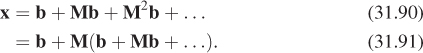
To keep things simple in what follows, and in analogy with the light-transport application we’ll soon examine, we’ll assume that all entries of M are nonnegative, the row-sum ri = Σj mij is less than 1 for all i, and the eigenvalues of M have magnitude less than 1, so that the series solution converges. We’ll also assume that M is an n × n matrix rather than just a 2 × 2 matrix.
Let’s use the ideas of the short programs above to estimate x1, the first entry of x in Equation 31.90. According to the equation, the value x1 is the sum of two numbers, b1 and (Mx)1. That makes it easy to find x1 using our sum-of-numbers estimator, but only if we already know x! But Mx1 is a sum: m11x1 + ... + m1nxn. We can estimate this by selecting among these terms at random, as usual. In each term, we know the mij factor, and we need to estimate the xj factor. So we can estimate x1 only if we can estimate xj for any j. This begs for recursion. And as is typical in recursion, the recursion gets easier if we broaden the problem. So we’ll write a procedure, estimate(i), that estimates the ith entry of x, and to find x1 we’ll invoke it for i = 1.
1 define estimate(i):
2 u = uniform(0, 1)
3 if (u > 0.5):
4 return bi / 0.5
5 else:
6 k = randint(1, n)
7 return mik· estimate(k) / (0.5 * (1/n))
The book’s website has actual code that implements this approach, and compares it with the answer obtained by actually solving the system of equations.
You’ll find, if you run it, that it works surprisingly well, at least when the eigenvalues are small, so that the series solution converges quickly.
For those who read the section on Markov chains, this program corresponds (when n = 2) to the Markov chain solution with all edges in the graph labeled with probability 0.5: When we’re in some state, half the time we terminate and half the time we make a recursive call, putting another factor of 0.5 in the denominator. Because the Markov chain version of the algorithm is guaranteed to produce a consistent estimator, this recursive version must do so as well. For the rest of this section, you can imagine how the recursive forms we write correspond to various Markov chain forms.
![]() Note that although this code is recursive, you can’t prove its correctness the same way you would prove that merge sort is correct, using induction: The recursive invocation of
Note that although this code is recursive, you can’t prove its correctness the same way you would prove that merge sort is correct, using induction: The recursive invocation of estimate is not “simpler” than the calling invocation, and there’s no base case. The structure of the code is recursive, but the analysis of it relies on the graph theory and Markov chains. In fact, the program’s not correct, at least not in the way that merge sort is correct. There’s an execution path (one where the random number u always turns out less than 0.5) in which the program executes forever, for instance! Nonetheless, with probability one the program produces an unbiased estimate of xi, which is all we can hope for with a Monte Carlo algorithm. (Recall from Chapter 30 that “probability one” does not mean certainty: There may be cases that fail, but they are as unlikely as picking, say, e/π when asked to choose a random number in the unit interval.)
Let’s now improve the algorithm in two ways. First, the values returned by estimate(1) tend to vary a lot: Half of them are 2b1 and the other half arise from a recursive call. We can get the same average result if we simply return b1 in all of them:
1 define estimate(i):
2 result = bi
3 u = uniform(0, 1)
4 if (u < 0.5):
5 k = randint(1, n)
6 result += mik· estimate(k) / (0.5 * (1/n))
7 return result
Now if mij is small for all j, then the recursive part of the code is likely to produce small results, because of the factor of mik. It would be nice, in this case, to bias our program toward skipping the recursive part.
Recall that we assumed that ri = Σj mij was less than one. That means we can change our code to
1 define estimate(i):
2 result = bi
3 u = uniform(0, 1)
4 if (u < ri):
5 k = randint(1, n)
6 result += mik· estimate(k) / (ri * (1/n))
7 return result
That’s the final version we’ll write for this particular problem. The use of ri corresponds, in the Markov chain model, to choosing greater or lesser values for pi3; the choice of k as a random integer between 1 and n could be improved a bit: We might, for instance, want to choose k with a probability proportional to mik. That would reduce variance, but it might also take longer. When we apply this technique to solving the rendering equation, we actually will do some clever things in that recursive part of the estimator. It just happens that in the matrix model of the computation, there’s no good analog for these subtleties.
Make certain you really understand every piece of the code in this section. Ask yourself things like, “Why is that 1/n in the denominator?” and “Why do we multiply by mik rather than mki?” Only proceed to the next section when you are confident of your understanding.
31.18.3. Building a Path Tracer
We’ll now describe how to build a path tracer in analogy with the recursive version of the linear equation solver, transforming a simple path tracer into one that’s increasingly tuned to use its sampling efficiently. The wrapper of the path tracer is quite simple:
1 for each pixel (x,y) on the image plane:
2 ω = ray from the eyepoint E to (x, y)
3 result = 0
4 repeat N times:
5 result += estimate of L(E, -ω)
6 pixel[x][y] = result/N;
There are variations on the wrapper. We could estimate the radiance through various points associated with pixel (x, y), and then weight the results by the measurement equation to get a pixel value. We could, for a dynamic scene, estimate the radiance at (x, y) for various different times and average them, generating motion-blur effects, etc. But all of these have at their core the problem of estimating L(E, –ω); we’ll concentrate on this from now on, writing a procedure called estimateL to perform this task.
The first version of the estimation code is completely analogous with the matrix equation solver: Because L is a sum of Le and an integral, we’ll use a Monte Carlo estimator to average the two terms. We’ll use the generic point C as the one where we’re estimating the radiance, but you should think of C as being the eyepoint E, at least until the recursive call.
Figure 31.23 shows the relevant terms. The red arrow at the bottom is Le(P, ω) (which for this scene happens to be zero, because the surface containing P is not an emitter).
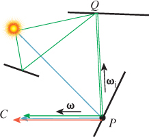
1 // Single-sample estimate of radiance through a point C
2 // in direction ω.
3 define estimateL(C, ω):
4 P = raycast(C, -ω) // find the surface this light came from
5 u = uniform(0, 1)
6 if (u < 0.5):
7 return Le(P, ω)/0.5
8 else:
9 ωi = randsphere() // unit vector chosen uniformly
10 integrand = estimateL(P, -ωi)· fs(P,ωi,ω)|ωi · nP|
11 density = ![]()
12 return integrand / (0.5 * density)
The choice of ωi uniformly on the sphere is analogous to choosing an index k = 1 ... n, except for one thing: When we chose k, it was possible that mik = 0, that is, the particular path we were following in the Markov chain would contribute nothing to the sum. But when we choose ωi, we’re going to estimate the arriving radiance at P in direction –ωi with a ray cast. We’ll then know that P is visible from whatever point happens to be sending light in that direction toward P. This was one of the great insights of the original path tracing paper: that using ray casting amounted to a kind of importance sampling for a certain integral over all surfaces in the scene. (Kajiya performed surface integrals rather than hemispherical or spherical ones.)
If the surface at P is purely reflective rather than transmissive, then half of our recursive samples will be wasted. Assume that transmissive(P) returns true only if the BSDF at P has some transmissive component. Rewrite the pseudocode above to only sample in the positive hemisphere if the scattering at P is nontransmissive.
Once again, we can replace the occasional inclusion of Le with an always inclusion. The code is then
1 define estimateL(C, ω):
2 P = raycast(C, -ω)
3 u = uniform(0, 1)
4 resultSum = Le(P, ω)
5 if (u < 0.5):
6 ωi = randsphere()
7 integrand = estimate(P, -ωi) * fs(P,ωi,ω)|ωi · nP|
8 density = ![]()
9 resultSum += integrand / (0.5 * density)
10 return resultSum
Now if we suppose that our BSDF can not only be evaluated on a pair of direction vectors, but also can tell us the scattering fraction (i.e., if the surface is illuminated by a uniform light bath, the fraction of the arriving power that is scattered), we can adjust the frequency with which we cast recursive rays:
1 define estimateL(C, ω):
2 P = raycast(C, -ω)
3 u = uniform(0, 1)
4 resultSum = Le(P, ω)
5 ρ = scatterFraction(P)
6 if (u < ρ):
7 ωi = randsphere()
8 Q = raycast(P, ωi)
9 integrand = estimate(Q, -ωi) * fs(P,ωi,ω)|ωi · n|
10 density = ![]()
11
12 resultSum += integrand / (ρ * density)
13 return resultSum
The second insight we’ll take from Kajiya’s original paper is that we can write the arriving radiance from Q as a sum of two parts: radiance emitted at Q (which we call direct light Ld at P), and radiance arriving from Q having been scattered after arriving at Q from some other point, which we call indirect light Li. Figure 31.24 shows these. There’s no direct light from Q to P in the figure, since Q is not an emitter, but there is direct light from R to P, shown in cyan. Notice that this division of light arriving at P from Q into different parts is a mathematical convenience. There’s no way, when a photon arrives at P from Q, to tell whether it was directly emitted or was scattered. But dividing the arriving light in this way allows us to structure our program to get better results.
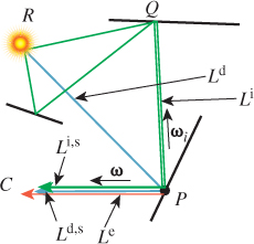
The figure also shows the results of scattering these at P, which we’ll call Ld,s and Li,s. The scattered radiance Lr is just Ld,s + Li,s. Thus,
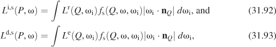
where Q = raycast(P, ω).
With these definitions, we restructure the code slightly (see Listing 31.5).
Listing 31.5: Kajiya-style path tracer, part 1.
1 define estimateL(C, ω):
2 P = raycast(C, –ω)
3 resultSum = Le(P, ω) + estimateLr(P, ω)
4 return resultSum
5
6 define estimateLr(P, ω):
7 return estimateLds(P, ω) + estimateLis(P, ω)
8
9 define estimateLis(P, ω): // single sample estimate
10 u = uniform(0, 1)
11 ρ = scatterFraction(P)
12 if (u < ρ):
13 ωi = randsphere()
14 Q = raycast(P, ωi)
15 integrand = estimateLr (Q, -ωi) * fs(P,ωi,ω)|ωi · n|
16 density = ![]()
17
18 return integrand / (ρ * density)
19 return 0
20
21 define estimateLds(...
Notice that in estimating the scattered indirect light, we didn’t scatter all the radiance arriving at P from Q, but only Lr. The Le portion of the radiance is the direct light, which we’re deliberately not including.
To estimate Ld,s (the scattering of the direct light), we are trying to evaluate the integral
where Q denotes the result of a ray cast from P in direction ωi.
We’re going to shift from a spherical integral to a surface integral (which involves the usual change of variable factor), and integrate over all light sources. (You should now think of Q as being a point on the light source in Figure 31.24.) To keep things simple, we’ll assume that we have only area light sources (no point lights!), and that there are K of them, with areas A1, ..., AK, and total area A = A1 + A2 + ... + AK.
The integral we want to compute is
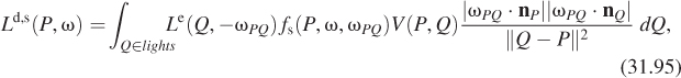
where ωPQ = S(Q – P) is the unit vector pointing from P to Q, and V(P, Q) is the visibility function, which is 1 if P and Q are mutually visible and 0 otherwise. (The extra dot product, and the squared length in the denominator, come from the change of variables.) Notice that in the integrand, we have Le and not L: We only want to estimate scattering of direct light.
We can estimate this integral by picking a point Q uniformly at random with respect to area (i.e., with probability Ai/A it’ll be a point of light i, and within light i, it’ll be uniformly randomly distributed), and using Q to perform a single-sample estimate of the integral:
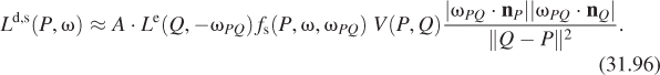
This makes the code for estimateLds fairly straightforward (see Listing 31.6).
Listing 31.6: Kajiya-style path tracer, part 2.
1 define estimateLds (P, ω):
2 Q = random point on an area light
3 if Q not visible from P:
4 return 0
5 else:
6 ωPQ = S(Q - P)
7 ![]()
8 return A · Le(Q, -ωPQ) fs (P, ω, ωPQ) · geom
Everything we’ve done here depends on the BSDF being “nice,” that is, having no impulses. In the next chapter, we’ll adjust the code somewhat to address that.
To summarize, path tracing works by estimating the integrand using a Markov chain Monte Carlo approach, including the reuse of initial segments of the chain for efficiency. It avoids the plethora of recursive rays generated by conventional ray tracing; the time saved is allocated to collecting multiple samples for each pixel. While path tracing is, in the abstract, an excellent algorithm, it does require that you choose an acceptance probability (we’ve used the scattering fraction) and a sampling strategy for outgoing rays; if these are chosen badly, the variance will be high, requiring lots of samples to reduce noise in the final image. Furthermore, the sampling strategy must be general enough to find all paths in your scene that actually transport important amounts of light. If you allow purely specular surfaces and point lights, then paths of the form LS+DE are problematic as mentioned above: The path starting from the eye must choose a direction, after the first bounce, that happens to be reflected one or more times to reach the point light. The probability of choosing this direction is unfortunately zero. If you allow nearly point lights and nearly specular reflections, you can still get the same effect: The probability of sampling a good path can be made arbitrarily small. To address this limitation, we have to consider other ways of sampling from the space of all possible light paths, or else take a great many samples to get a good estimate (i.e., a low-noise image).
What’s the difference between a path tracer and a conventional ray tracer? Well, the path-tracing result tends to be noisy, as we mentioned earlier: We’re making Monte Carlo estimates of the radiance at each point, and there’s variance in these estimates. A basic ray tracer that only computes recursive rays when there’s a mirror reflection uses a very low-variance estimate of the diffusely scattered indirect light: It estimates it as zero! That makes the basic ray-traced image darker than it should be, but uncluttered with noise. On the other hand, by taking more samples in the path tracer, we can reduce the noise a lot. For a small ray-casting budget (i.e., you can only afford to cast a certain number of rays in your scene), the simple ray-tracer result is wrong but nice looking; the path-traced result is generally “right on average,” but noisy. As the ray-casting budget increases, the ray-traced result does not really improve (except for deeper levels of reflection), while the path-traced result gets less and less noise, and correctly includes diffusely scattered indirect light.
Finally, we’ve treated “measurement” as part of the wrapper for a path tracer, but we could instead include it in the thing being computed, so rather than estimating L, we could estimate L multiplied by the measurement function M. When we do so, the thing we’re integrating, expanded out recursively, is a product of some number of scattering functions and cosines, an Le at the end, and M at the beginning. (If we’re integrating with respect to area rather than solid angle, there will also be some change-of-variables factors.) There’s a symmetry in this formulation: We could swap the roles of M and Le, and imagine rendering a scene in which the eye was emitting light according to M, and it was being measured at the light sources using Le as the measurement function. The integral we’d write down for estimating light transport in this “swapped” scene would be exactly the same as in the original. This provides some theoretical justification for the “trace rays from the eye” approach rather than tracing photons from the lights, the way nature does it: The integrals we’re estimating are the same.
31.18.4. Multiple Importance Sampling
When we consider alternative ways to sample from the space of light paths, we may find one sampling strategy that is effective for one class of paths and another that works well for a different class. It’s difficult to know in advance which will be useful in any particular scene. Veach developed multiple importance sampling as a way to use many different sampling strategies in evaluating a single integral, by weighting samples from the different strategies differently. He describes a motivating example: a single glossy surface reflecting an area light source (e.g., think of a slightly rippled ocean reflecting moonlight). In this case, there are only two interesting kinds of paths: LE and LDE; if the lights are outside the visible part of the scene, then there are only LDE paths. There are no paths of length greater than two in the scene. This makes the analysis particularly easy. We’ll look at only the LDE paths.
Suppose that we try to estimate the light arriving at some pixel, P. One approach to sampling paths is that we trace a ray through P, meeting the glossy surface at a point x. Then we sample from the BRDF at x and trace a second ray that may hit the area light source, in which case the sample contributes some radiance, or that may miss the light altogether, in which case the sample contributes zero. An alternative approach is to trace the ray through P to x, but then sample a point x′ uniformly at random on the light source, and connect x to x′. Now the path certainly carries some radiance.
The second approach initially seems far better than the first approach, since the paths will always conduct some light. But what if the surface is very rough? Then the BRDF in the xx′ direction may be nearly zero, and so the contribution is again very small. Figure 31.25 shows the results in practice.
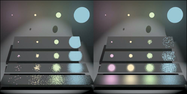
Figure 31.25: The image on the left was made by sampling the BRDF of the rough surface; the nearer slabs are rougher than the distant ones. Four light sources of varying sizes produce different glossy reflections. The image on the right used sampling on the light sources. The upper right in the first picture is preferable to that in the second; the lower left in the second picture is preferable to that in the first. No one sampling strategy is best. (Note that the scene is also lit by a weak light above the camera, and that the slabs all have a small diffuse component, letting us see their general shapes.) (Courtesy of Eric Veach.)
Clearly we want to use one sampling strategy in estimating the integral in some cases, the other in other cases, and a mix of the two in still other cases. This is where multiple importance sampling comes in. Before we discuss that, there’s one point worth noting: If you have two estimators, one with large variance and one with small variance, and you average them, you’re in trouble: It’s really hard to get rid of the variance except by taking lots of samples. Informally speaking, the central idea of multiple importance sampling is that it provides a way to work with a kind of average of two estimators without letting the larger variance of one of them creep into the later computations.
To describe multiple importance sampling, we return to the abstract setting: We’re trying to integrate a function f on some domain D, and we have two different sampling methods that produce samples X1, j, j = 1, 2, ... and X2, j, j = 1, 2, ... with density functions p1 and p2, respectively.
To estimate the integral using samples from the two different distributions, we need only produce two weighting functions, w1 and w2, from D to R, with two properties:
• w1(x) + w2(x) = 1 for any x with f (x) ≠ 0.
• w1(x) = 0 whenever p1(x) = 0, and similarly for w2 and p2.
It generally makes sense for both weighting functions to be non-negative, in which case both vary between zero and one.
As a trivial example, at least in the case where each pi is nonzero everywhere on the domain, we could pick w1(x) = 0.25 for every x, and w2(x) = 0.75 for every x. But more interesting cases arise when the weights are allowed to vary as a function of the samples. We’ll return to this in a moment.
Once we have chosen weighting functions, we take n1 samples of X1,j from the first distribution, and n2 samples from the second, and combine them in the multisample estimator given by
Veach shows that the multisample estimator F is in fact unbiased, and that with suitably chosen weights, it has good variance properties. (An exactly analogous formula works for three, four, or more samplers.)
What are good weight choices? The naive constant-weight approach is one; another is closely related: If we partition the domain D into two subsets D1 and D2 with D1 ![]() D2 = D and D1
D2 = D and D1 ![]() D2 =
D2 = ![]() , we can define wi(x) = 1 when x
, we can define wi(x) = 1 when x ![]() Di, and 0 otherwise. This effectively says, “Use one kind of sampling on each part of the domain.” One application of this is when we partition the space of paths into, for instance, those with zero, one, two, ...specular bounces, and use a different sampler for each. Another is when we’re sampling from a Phong-style BRDF and have to choose between a specular, a glossy, and a diffuse reflection.
Di, and 0 otherwise. This effectively says, “Use one kind of sampling on each part of the domain.” One application of this is when we partition the space of paths into, for instance, those with zero, one, two, ...specular bounces, and use a different sampler for each. Another is when we’re sampling from a Phong-style BRDF and have to choose between a specular, a glossy, and a diffuse reflection.
31.18.5. Bidirectional Path Tracing
Path tracing makes its choice about extending paths based on the current point (i.e., selectRay is a function of only xk). But the actual lighting in a scene may matter as well: If a bright light shines on a dark surface, considerable light may still be reflected. And lots of dim rays reflected even from a low-reflectance surface may converge to form caustics which are perceptually significant. In recognition of this, Lafortune and Willems [Laf96] and Veach [VG94] independently proposed bidirectional path tracing, in which paths are traced both from light sources and from the eye. At a naive level, this sounds implausible: There’s essentially no chance that two such paths will ever land on the same point so that light is carried all the way from the luminaire to the eye! But a simple trick (see Figure 31.26) addresses this difficulty: We join the two paths with a segment! In fact, we can join any point on the first path to any point on the second path with such a segment, and compute the total transport along the resultant path.
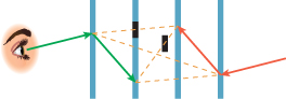
Figure 31.26: A path is traced from the light and the eye; each point of the first path is connected to each point of the second to create paths from the luminaire to the eye. These connecting segments may, however, meet occluders (shown as black segments), creating no net transport.
While the light-path and eye-path segments are all generated by tracing rays, and hence are guaranteed to transport light, the joining segments may meet occluders that make them transport no light at all. This potential occlusion can waste a great deal of path-tracing time and increase the variance of the pixel estimates. When the joining segment is not occluded, the computation of the contribution of the resultant path to the total transport is also very complex.
In practice, however, bidirectional path tracing tends to produce quite good results, good enough that they can (with enough samples) be used as a reference standard for evaluating other rendering methods.
To use the traced paths as samples for estimating the integral in the rendering equation, we need to know not only the transport along the path, but also the probability of having generated the path. Computing this probability requires careful analysis of the program used to generate the paths: How likely are we to have generated the two spliced-together subpaths? How likely are we to have spliced the paths together along this particular edge? These probabilities depend on the sampling approach. For instance, to generate a path, we might do one of the following.
• Repeatedly cast a ray in a uniform random direction (i.e., the probability that the direction lies in some solid angle is proportional to the measure of that solid angle) in the outgoing hemisphere from the current path point.
• Repeatedly cast a ray uniformly with respect to the projected solid angle.
• Repeatedly choose a point (toward which we’ll cast a ray) at random with respect to the area on the union of all surfaces in the scene.
Each of these will sample some paths more often than others; switching from one to another is similar to changing variables in an ordinary integration problem: An extra factor is introduced in the integrand. And while the geometry term for the “choosing surface points” version has a ![]() factor, which leads to very large values when two chosen points are close to each other (see Figure 31.27), in the “choosing directions” version this change of variables exactly cancels out the bad factor in the geometry term, except for the factor associated with the edge joining the light path to the eye path.
factor, which leads to very large values when two chosen points are close to each other (see Figure 31.27), in the “choosing directions” version this change of variables exactly cancels out the bad factor in the geometry term, except for the factor associated with the edge joining the light path to the eye path.
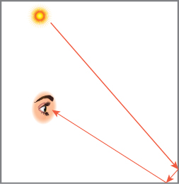
Figure 31.27: If this light path is chosen by selecting points uniformly on surfaces, it will contribute a large value to the integral because of the short segment in the corner and the ![]() term in the integrand.
term in the integrand.
Veach describes how multiple importance sampling can be used to ameliorate this problem.
31.18.6. Metropolis Light Transport
In 1997, Veach and Guibas [VG97] described the Metropolis light transport, or MLT, algorithm. This was yet another Markov chain Monte Carlo approach, but the Markov chain no longer formed a random walk in the set ![]() of all surface points in the scene, as it did in the path-tracing algorithms; instead, the algorithm takes a random walk in the space of all paths in the scene. That is to say, the algorithm may first examine a path of length 1, then a path of length 20, then a path of length 3, etc. Explicitly describing this space of paths, and how to randomly sample from it, is difficult. There’s also the unfortunate fact that the Metropolis-Hastings algorithm, on which MLT is based, only provides a result that’s guaranteed to be proportional to the result you’re seeking. Fortunately in MLT, we’re seeking a whole array of results (the output pixel values), and the constant of proportionality is the same for all of them. In other words, we get an image that’s some constant multiple of the desired image. But once again, there’s bad news: The constant of proportionality may be zero, that is, we may get an all-black image. Finally, while MLT’s result is guaranteed to be unbiased, it may take a great many paths to ensure that the variance is low (just as with other Monte Carlo methods); the rapidity of variance reduction depends, in part, on how cleverly one chooses a mutation strategy, which determines how new paths are generated from the current one. (This is closely analogous to what we saw in computing sums of matrix powers: Picking the transition probabilities pij dramatically affected the rate of convergence.) Thus, once you develop an MLT renderer, you can improve upon it by adding more and better mutation strategies; such mutation strategies are ways to express your knowledge of the structure of light transport. That is to say, you might argue that if lots of light is being carried along this path, then if you only move the eye ray a tiny bit, which moves the first interior point of the path, but you leave everything else the same, maybe the new path will also carry lots of light. The nature of the algorithm makes it easy to express this kind of high-level understanding.
of all surface points in the scene, as it did in the path-tracing algorithms; instead, the algorithm takes a random walk in the space of all paths in the scene. That is to say, the algorithm may first examine a path of length 1, then a path of length 20, then a path of length 3, etc. Explicitly describing this space of paths, and how to randomly sample from it, is difficult. There’s also the unfortunate fact that the Metropolis-Hastings algorithm, on which MLT is based, only provides a result that’s guaranteed to be proportional to the result you’re seeking. Fortunately in MLT, we’re seeking a whole array of results (the output pixel values), and the constant of proportionality is the same for all of them. In other words, we get an image that’s some constant multiple of the desired image. But once again, there’s bad news: The constant of proportionality may be zero, that is, we may get an all-black image. Finally, while MLT’s result is guaranteed to be unbiased, it may take a great many paths to ensure that the variance is low (just as with other Monte Carlo methods); the rapidity of variance reduction depends, in part, on how cleverly one chooses a mutation strategy, which determines how new paths are generated from the current one. (This is closely analogous to what we saw in computing sums of matrix powers: Picking the transition probabilities pij dramatically affected the rate of convergence.) Thus, once you develop an MLT renderer, you can improve upon it by adding more and better mutation strategies; such mutation strategies are ways to express your knowledge of the structure of light transport. That is to say, you might argue that if lots of light is being carried along this path, then if you only move the eye ray a tiny bit, which moves the first interior point of the path, but you leave everything else the same, maybe the new path will also carry lots of light. The nature of the algorithm makes it easy to express this kind of high-level understanding.
Furthermore, there are some mutation strategies that are relatively easy to implement, but which end up more frequently sampling a “bright” area of the path space that’s previously been rarely sampled. Such strategies represent a big improvement in the algorithm.
The details of the algorithm are, unfortunately, rather complex, and involve substantial mathematics. The reader interested in reproducing the results should read Veach’s dissertation [Vea97]; indeed, anyone really interested in rendering should do so.
31.19. Photon Mapping
Recall that we described photon mapping as being like bidirectional path tracing, except that rather than connecting an eye path to a light path, we took the final point, P, of the eye path and used the collection of all the light paths to estimate the light arriving at P. The problem, of course, is that in any finite set of light paths, there aren’t likely to be any that end exactly at P. Instead, we have to estimate the arriving light by looking at the arriving light at nearby points and interpolating somehow.
Doing so entails representing all the arriving light in such a way that searching for “nearby” points is easy. In photon mapping, this incoming light is stored in a photon map, a relatively compact structure that’s not directly related to the scene geometry. Information in the map is stored at points; we’ll describe exactly the data stored at each point presently.
Thus, photon mapping has two phases: the construction of the photon map (via photon tracing), and the estimation of the outgoing radiance (at many different points) using the photon map.
The process of estimating the radiance leaving a surface from the knowledge of the radiance arriving at several nearby points involves scattering the arriving light (via the BSDF). One advantage of storing the arriving light (or at least a sample of the arriving light) is that it compactly represents a great many outgoing light rays (via the BSDF). A sample of the arriving light is stored in a record that’s unfortunately called a photon, despite being quite distinct from the elementary particle of the same name. A photon-mapping photon (which is the only kind we’ll discuss in the remainder of this section) consists of a location in space, a direction vector ωi that points toward the light source or the last bounce the light took before arriving at this point (i.e., ωi points opposite the direction of propagation), and an incident power. It’s helpful to assign units: The coordinates of the location should be specified in meters; the direction vector is unitless, but has length 1; and the power is specified in watts. We’ll denote these by P, ωi, and Φi, respectively. A photon-mapping photon therefore represents an aggregate flow of many physical photons per second.
The scene represented by the photon map consists of surfaces and luminaires (which may themselves be surfaces). For each light L we let ΦL be the emissive power of the light. For example, a 40 W incandescent lamp has an emissive power of about 10 W in the visible spectrum, so for such a bulb, ΦL = 10 W. And we denote the total power of all light sources by
Surfaces in the scene have a BSDF fs(P, ωi, ωo) at each point P of the surface. Because the BSDF may vary with wavelength, we include a fourth parameter: fs(P, λ, ωi, ωo), with the understanding that λ may represent an actual wavelength, or it may (as in most implementations) represent a band of wavelengths, where the bands are typically denoted by the symbols R, G, and B. The same applies to ΦL and Φ: Each depends on wavelength. For all three, the omission of the wavelength parameter indicates summation. For instance,
Photon mapping has, in addition to the scene description, two main parameters: N, the total number of photons to be “shot” from the light sources, and K, the number of photons to be used in estimating the outgoing radiance at any point. The value N is used only in the construction of the photon map; the value K only in the radiance estimation. A third parameter, maxBounce, limits the number of bounces that a photon can take during the photon-tracing phase of the algorithm.
The photon map itself is a k-d tree storing photons, using the position of the photon as the key. Listing 31.7 shows how the photon map is constructed.
Listing 31.7: Constructing a photon map via photon tracing.
1 Input: N, the number of photons to emit,
maxBounce, how many times a photon may be reflected
a scene consisting of surfaces and lights.
Output: a k-d tree containing many photons.
2
3 define buildPhotonMap(scene, N, maxBounce):
4 map = new empty photon map
5 repeat N times:
6 ph = emitPhoton(scene, N)
7 insertPhoton(ph, scene, map, maxBounce)
8 return map
9
10 define emitPhoton(scene, N):
11 from all luminaires in the scene, pick L with probability
12 p = ΣλΦL(λ)/ΣλΦ(λ).
13
14 ph = a photon whose initial position P is chosen uniformly
15 randomly from the surface of L, whose direction ωi
16 is chosen proportional to the cosine-weighted radiance at P in
17 direction ωi, and with power Φi = ΦL/(Np).
18
19 define insertPhoton(ph = (P, ωi, Φi), scene, map, maxBounce)
20 repeat at most maxBounce times:
21 ray trace from ph.P in direction ph.ωi to find point Q.
22 ph.P = Q
23 store ph in map
24 foreach wavelength band λ:
25 pλ = ∫fs(Q,λ,ωi,ωo)ωo · n dωo, probability of scattering.
26 ![]() = average of pλ over all wavelength bands λ.
= average of pλ over all wavelength bands λ.
27 if uniform(0, 1) > ![]()
28 // photon is absorbed
29 exit loop
30 else
31 ωo = sample of outgoing direction in proportion to fs(Q,ωi,·)
32 ph.ωi = -ωo
33 foreach wavelength band λ:
34 ph.Φi(λ) * = pλ/![]()
Most of this is a straightforward simulation of the process of light bouncing around in a scene. If, for a moment, we ignore wavelength dependence, then the absorption step can be explained, just as we saw in path tracing, as follows: When a photon hits a surface that scatters 30% of the arriving light, we could produce a scattered photon with its power multiplied by a factor of 0.3, or we could produce a scattered photon will full power, but only 30% of the time, an approach called Russian roulette. Over the long term, as many photons arrive at this point and get scattered, the total outgoing power is the same, but there’s an important difference between the two strategies: In the second, at least for a scene that is not dependent on wavelength, the power of a photon never changes. This means that all samples stored in the photon map have the same power. This makes the radiance-estimation step work better in general, although the statistical reasons for that are beyond the scope of this book. The code, in saying “reflect a full-strength photon with a probability determined by the scattering probability,” is applying Russian roulette.
Because the scattering is wavelength-dependent, the final update to Φi(λ) scales the power in each band in proportion to that band’s scattering probability. Notice that if the surface is white (i.e., reflectance is the same across all bands), then Φ(λ) is unchanged. By contrast, if we’re using RGB and the surface is pure red, then the average scattering probability is 1/3; the red component of the photon power is multiplied by ![]() , while the green and blue components are set to zero.
, while the green and blue components are set to zero.
What happens to the power of a photon if the surface is a uniform 30% gray, so it reflects 30% of the light at each wavelength?
The actual implementation of light emission and of scattering (particularly for reflectance models that have a diffuse, a glossy, and a specular part, for instance) requires some care; we discuss these further in Chapter 32.
The second part of photon mapping is radiance estimation at points visible from the eye, determined, for instance, by tracing rays from the eye E into the scene. Before performing any radiance estimation, however, we balance the k-d tree. Then for each visible point P, with normal n, we let ωo = S(E – P), and compute the radiance.
1. Set L = 0 W/m2sr. L represents the radiance scattered toward the eye.
2. Find the K photons nearest to P in the photon map, by searching for a radius r within which there are K photons.
3. For each photon ph = (Q, ωi, Φi), update L using
where ![]() is called the estimator kernel. This assignment is wavelength-dependent (i.e., if we use three different wavelength bands, Equation 31.100 represents three assignments, one for each of R, G, and B).
is called the estimator kernel. This assignment is wavelength-dependent (i.e., if we use three different wavelength bands, Equation 31.100 represents three assignments, one for each of R, G, and B).
It’s easy to see that this computation is an approximation of the integral ∫ fs(P, ωi, ωo)ωi · n dωi over the positive hemisphere at P: The arriving radiance at nearby points is used as a proxy for the arriving radiance at P in the integral. Of course, light arriving at some point Q that’s near P from direction ωi may have originated at a fairly nearby light source. If so, then the arriving direction at Q will be different from that at P (see Figure 31.28).
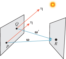
Figure 31.28: Light from the sun arrives at P from some direction η; sunlight will also arrive at Q from almost exactly that direction. But if light from a nearby point R arrives at P in direction ω, that same source will provide light at Q from direction ω′ which may not be close to ω.
Furthermore, it’s possible that some light is visible from point P but shadowed at point Q, in which case the use of the incoming light at Q in estimating the incoming light at P is inappropriate. It is for this reason that photon mapping is biased: Without infinitely many photons, some points in dark areas will get their radiance estimates in part from photons in lighter areas, biasing them toward brighter estimates.
On the other hand, at least at points of diffuse surfaces, photon mapping is consistent: As the number of photons, N, goes to infinity, the K samples used to estimate the light arriving at P are closer and closer to P, causing the incoming directions to be increasingly better approximations of the incoming direction at P, and the radiances to be increasingly better approximations of the radiances at P.
The preceding analysis of consistency assumed that K was held constant while N goes to infinity. Is the analysis still valid if K is set to a constant multiple of N, say, K = 10–5N? Why or why not?
Estimating arriving radiance from nearby samples works best when the arriving radiance varies smoothly as a function of both position and angle. When there are point lights and sharp edges in the scene, we get hard shadows, which makes the arriving radiance discontinuous. On the other hand, this nonsmoothness in arriving radiance is primarily a consequence of direct lighting, that is, light paths of the form LDE. We can therefore divide the domain of the integral in the rendering equation into two parts: those paths of the form LDE, and all other paths. We can estimate the integral as a sum of the integrals over each part. The first part is relatively easy: Single-bounce ray tracing suffices to estimate the direct lighting at every point of the scene. What about the second part? We can estimate that using photon mapping! But to do so, we need to eliminate any estimate of transport of the form LDE from the photon map. We do so by slightly modifying the construction of the photon map: For each of the N photons, we record in the photon map only the second and subsequent bounces.
Photon mapping has other limitations. Because points that are nearby in space may not be nearby in surface normal (see Figure 31.29), using all nearby photons can give erroneous estimates. Several heuristics have been applied to mitigate this problem [Jen01, ML09].
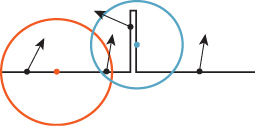
Figure 31.29: Estimating arriving radiance with nearby photons works badly at corners and near thin walls.
When we use the constant kernel κ(v) = 1/(πr2), we have the problem that as the point at which we’re estimating radiance moves, we typically lose one photon at one side of the moving disk and gain another somewhere on the other side; if these two photons have different power vectors (power in each wavelength band), then the radiance estimate can have discontinuities, which appear as noticeable artifacts in the final results. Alternative kernels can mitigate this somewhat, as Jensen describes.
What we’ve described is the basic form of photon mapping presented in Jensen’s book, but there are many implicit parameters in the description. For instance, the k-d tree used for storing photons can be replaced by other data structures like spatial hashing [MM02], the kernel used for density estimation can be varied, and even the density estimation technique itself can be altered.
31.19.0.1. Final Gathering
One particularly effective enhancement is use of a “final gathering” step during density estimation. When we examine a point P in the scene, we can estimate the field radiance at P either by looking at its nearest neighbors, as we’ve described, or by shooting lots of rays from P to hit other points, Qi(i = 1, 2, ...), and then using nearest-neighbor techniques to estimate the field radiance at each Qi, and the light reflected back toward P from each Qi. The collection of these gathered lights is also a valid estimate of the field radiance at P, but is much less likely to exhibit the discontinuities described above, as any discontinuity is typically averaged with a great many other continuous functions.
31.19.1. Image-Space Photon Mapping
McGuire and Luebke [ML09] have rethought photon mapping for a special case—point lights and pinhole cameras—by recognizing that in this case, some of the most expensive operations could be substantially optimized. One of these operations—the transfer of information from photons in the photon map to pixels in the image—is highly memory-incoherent in the original photon-mapping algorithm: One must seek through the k-d tree to find nearby photons, and depending on the memory layout of that tree, this may involve parts of memory distant from other parts. On the other hand, if every photon, once computed, could make its contribution to all the relevant pixels (which are naturally close together in memory), there would be a large improvement. The resultant algorithm is called image-space photon mapping. This approach harkens back to Appel’s notion of drawing tiny “+” signs on a plotter: These marks were spatially localized, and hence easy to draw with a plotter. It’s also closely related to progressive photon mapping [HOJ08], another approach that works primarily in image space.
The key insight is that when we ray-cast into the scene to gather light from photons, adjacent pixels are likely to gather light from the same photons; we could instead project the photons onto the film plane and add light to all the pixels within a small neighborhood. There are quite a few subtleties (How large a neighborhood? What about occlusion?), but the algorithm, implemented as a CPU/GPU hybrid, is much faster than ordinary photon mapping. While the algorithm only works with point lights and pinhole cameras, the added speed may be sufficient to justify this limitation in some applications such as video games.
31.20. Discussion and Further Reading
Many of the ideas in this chapter have been implemented in the open-source Mitsuba renderer [Jak12]. Seeing such an implementation may help you make these ideas concrete (indeed, we strongly recommend that you look at that renderer), but we also recommend that you first follow the development of the next chapter, in which some of the practical little secrets of rendering, which clutter up many renderers, are revealed. This will make looking at Mitsuba far easier.
While much of this chapter has been about simulation of light transport, there are a few large-scale observations about light in scenes that have crept into the discussion in disguise. We now revisit these in greater detail.
For instance, in classifying light paths using the Heckbert notation, we effectively partition the space of paths into subspaces, each of which we consider differently. We know, for instance, that much of the light in a scene is direct light, carried along LDE paths, and that in a scene with point lights and hard-edged objects, this direct light contains many of the discontinuities in the light field (corresponding to silhouettes, contours, and hard shadows).
The partitioning by Heckbert classes is useful, but rather coarse: Paths with multiple specular bounces may have high “throughput,” but this only matters if they start at light sources. There may someday be other ways of classifying paths that allows us to delimit the “bright parts” of path space more efficiently.
As we consider computing the reflectance integral at some point, it’s reasonable to ask, “How much do the variations in the field radiance matter?” If the surface is Lambertian, the answer is, “Generally not too much.” If it’s shiny, then variations in field radiance matter a lot. But having computed the reflectance integral to produce surface radiance, which may have considerable variation with respect to outgoing direction, we can ask, “When this arrives at another surface, how will that variation appear?” If we look at such a surface up close, moving our eyes a few centimeters may yield substantial variation in the appearance of the surface. But if we look at the same surface from a kilometer away, we’ll have to move our eyes dozens of meters to see the same variation. This dispersal of high-frequency content in the light field (and other related phenomena) is discussed by Durand et al. in a thought-provoking paper [DHS+05] that ties together the frequency content of the radiance field, both in spatial and angular components, with ideas about appropriate rates for sampling in various rendering algorithms.
We’ve treated rendering as a problem of simulating sensor response to a radiance field, with the implicit goal of getting the “right” sensor value at each pixel. This may not always be the right goal. If the image is for human consumption, it’s worth considering the end-to-end nature of the process, from model all the way to percept. Humans are notorious, for instance, for their inability to detect absolute levels of almost any sensation, but they are generally quite sensitive to variation. We can’t tell how bright something is, but we can reliably say that it’s a little brighter than another thing that’s near it, for instance. This means that if you had a choice between a perfect image, corrupted by noise so that a typical pixel’s value was shifted by, say, 5%, and the same perfect image, with every pixel’s value multiplied by 1.1, you’d probably prefer the second, even though the first is closer to the perfect image in an L2 sense.
Indeed, the human eye, while sensitive to absolute brightness, is much more sensitive to contrast. It might make sense, in the future, to try to render not the image itself, but rather its gradients, perhaps along with precise image values at a few points. The “final step” in such a rendering scheme would be to integrate the gradients to get an intensity field, subject to the constraints presented by the known values; such a constrained optimization might better capture the human notion of correctness of the image. We are not proposing this as a research direction, but rather to get you thinking about the big picture, and what aspects of that big picture current methods fail to address.
We’ve concentrated on the operator-theoretic solution of the rendering equation, but we’ve by no means exhausted these approaches. The solution says that (I – T)– 1e = (I + T + T2 + ...)e, where e describes the luminaires in the scene. If we slightly rewrite the right-hand side, we can discover other approaches based on this solution:
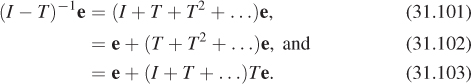
This says that aside from light reaching the eye directly from luminaires (the first e term), we can instead apply the transport operator once to the luminaires (Te) to get a new set of luminaires which we can then render using the series solution (I + T + ...). This is the key idea in an approach called virtual point lights [Kel97]: The initial transport of the luminaires is performed by something very similar to photon tracing, except that instead of recording the field radiance at the intersection point, we record the resultant surface radiance after scattering. This surface radiance becomes one of the virtual point lights (or, in image-space photon mapping, the bounce map).
If, following Arvo, we further decompose T into the product KG, where G transports surface radiance at each point to field radiance at another, and K scatters field radiance at a point into surface radiance there, then we can consider breaking a term off the series solution in a slightly different way:
In this form, we transport the radiance from the luminaires to become field radiance at the other surfaces in the scene (Ge). Subsequent processing involves tracing rays from the eye to various depths, and then scattering (the K term) the field radiance we find at intersection points. This can be regarded as a primitive form of photon mapping, in which the photon map contains only one-bounce photons.
Doubtless other factorizations of the series solution can lead to further algorithms as well.
This chapter has merely given a broad view of some topics in rendering, focusing attention on Monte Carlo methods because of our belief that these are likely to remain dominant for some time. To paraphrase Michael Spivak [Spi79b], we’ve introduced you to much of the foundational material, and “beyond all this lies a vast porridge of literature, and [we are] not glutton[s] enough to pick out all the raisins.”
If you want to know more about the physical and mathematical basis of rendering, and especially Monte Carlo methods, we recommend Veach’s dissertation [Vea97] as an education in itself. For those for whom the assumptions that lie at the foundation of rendering are important, Arvo’s dissertation [Arv95] is an excellent starting point, particularly for the operator-theoretic point of view. Both, however, involve considerable mathematics. The SIGGRAPH course notes [JAF+01] give a slightly less demanding transition.
On the other hand, if efficient approximations to the ideal interest you, then Real Time Rendering [AMHH08] is an excellent reference.
For modern implementations of Monte Carlo methods, Phyiscally Based Rendering by Pharr and Humphreys [PH10] is detailed and comprehensive.
Most important, the best place to start is with current research in the field. Research in rendering is featured at almost every graphics conference. The Eurographics Symposium on Rendering deserves special mention, however, as its long-term focus on rendering has made it a particularly fertile ground for new ideas. We suggest that you grab a paper, start reading and chasing references, and be both open-minded and skeptical at all times.
It’s also interesting to ask yourself, “What remains to be done?” Do current images lack realism because the modeling of materials is inadequate? Because certain classes of light paths are not being sampled? Because we aren’t using enough spectral bands? Because important information is contained in high-bounce-count paths, even though very little light energy is there? Probably all of these matter to some degree. At the same time, we make some assumptions (the “ray optics” assumption, for one) that limit the phenomena we can hope to capture faithfully. Do these matter? How important is diffraction? How important are wave optics phenomena in general? Questions like these will be the foundation of future research in rendering.
31.21. Exercises
Exercise 31.1: Suppose that tracing a ray in your scene takes time A on average, while evaluating the BRDF on a pair of vectors takes time B. (a) In tracing N rays from the eye using path tracing, using a fixed attenuation rate r (so that a path is extended at each point with probability (1 – r)), estimate the time taken in terms of A and B (assume all other operations are free).
(b) Consider tracing N/2 rays from the eye and N/2 rays from the single light source in a scene using bidirectional path tracing; do the same computation.
Exercise 31.2: The radiosity equation
has the form Mb = e, where M = I – F. In practice, the largest eigenvalue or singular value of M is considerably less than 1.0; this means that powers of M tend to grow rapidly smaller. That can be used to solve the equation relatively quickly.
(a) Show that (I – F)– 1 = I + F + F2 + ... by multiplying the right-hand side by I – F and canceling. This sort of cancellation is valid only if the right-hand side is an absolutely convergent series; fortunately, if the eigenvalues or singular values are small, it is, justifying this step.
(b) Show that
(c) Letting b0 = e and b1 = e + Fb0, and generally letting bk = e + Fbk–1, show that bk is the sum of the first k + 1 terms of the right-hand side of the equation for b, and that thus bk ![]() b as k
b as k ![]() ∞. Thus, an algorithm for computing the radiosity vector b is to start with b = e, and then multiply by F and add e repeatedly until b has converged sufficiently.
∞. Thus, an algorithm for computing the radiosity vector b is to start with b = e, and then multiply by F and add e repeatedly until b has converged sufficiently.
(d) If we think of the ith entry of b as the radiosity at patch i, then multiplying by F distributes this radiosity among all other patches. Rather than computing Fb in its entirety, which can involve lots of multiplication, we can push the “unshot” radiosity from a single patch through the matrix. Various algorithms exploit this idea, seeking, for example, to push through the matrix the largest unshot radiosity. Implement one of these for a 2D radiosity model, and see how its runtime and convergence compare with the naive algorithm that multiplies b by all of F at each step.
Exercise 31.3: Final gathering in photon mapping involves sampling from the hemisphere at a point P where we’re trying to estimate field radiance. As we move from point to point, our varying choice of samples will introduce noise into the estimates. Argue both for and against a strategy in which we choose, once and for all, a fixed collection of directions to use in the final gathering step.