
Chapter 11. Transformations in Three Dimensions
11.1. Introduction
Transformations in 3-space are in many ways analogous to those in 2-space.
• Translations can be incorporated by treating three-dimensional space as the subset E3 defined by w = 1 in the four-dimensional space of points (x, y, z, w). A linear transformation whose matrix has the form 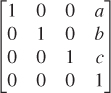 , when restricted to E3, acts as a translation by [a b c]T on E3.
• If T is any continuous transformation that takes lines to lines, and O denotes the origin of 3-space, then we can define
and the result is a line-preserving transformation ![]() that takes the origin to the origin. Such a transformation is represented by multiplication by a 3 × 3 matrix M. Thus, to understand line-preserving transformations on 3-space, we can decompose each into a translation (possibly the identity) and a linear transformation of 3-space.
that takes the origin to the origin. Such a transformation is represented by multiplication by a 3 × 3 matrix M. Thus, to understand line-preserving transformations on 3-space, we can decompose each into a translation (possibly the identity) and a linear transformation of 3-space.
• Projective transformations are similar to those in 2-space; instead of being undefined on a line, they are undefined on a whole plane. Otherwise, they are completely analogous.
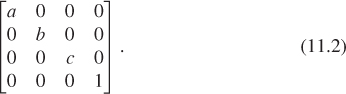
• Scale transformations can again be uniform or nonuniform; those that are nonuniform are characterized by three orthogonal invariant directions and three scale factors rather than just two, but nothing else is significantly different. The matrix for an axis-aligned scale by amounts a, b, and c along the x-, y-, and z-axes, respectively, is
Scale transformations in which one or three of a, b, and c are negative reverse orientation: A triple of vectors v1, v2, v3 that form a right-handed coordinate system will, after transformation by such a matrix, form a left-handed coordinate system. A uniform scale by a negative number has all three diagonal entries negative, and hence reverses orientation.
• Similarly, shearing transformations continue to leave a line fixed. Points not on this line are moved by an amount that depends on their position relative to the line, but this position is now measured in two dimensions instead of just one. There are also shears that leave a plane fixed.
• Reflections in 2D were either reflections through a point (the transformation x ![]() –x), which turns out to be the same as rotation by an angle π, or reflections through a line. In 3D, there are reflections through a point, a line, or a plane. Reflection through a line corresponds to rotation about the line by π. Reflection through a point is still given by the map x
–x), which turns out to be the same as rotation by an angle π, or reflections through a line. In 3D, there are reflections through a point, a line, or a plane. Reflection through a line corresponds to rotation about the line by π. Reflection through a point is still given by the map x ![]() –x; in contrast to the two-dimensional case, this map is orientation-reversing. Finally, reflection through a plane is given by the map
–x; in contrast to the two-dimensional case, this map is orientation-reversing. Finally, reflection through a plane is given by the map
where n is the unit normal vector to the plane. This is algebraically analogous to reflection through a line in two dimensions, but in three dimensions it is orientation-preserving. The matrix for this map is
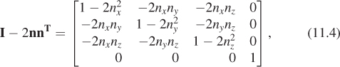
but it should come as no surprise at this point that we recommend that you use the expression I – 2nnT to create a reflection matrix rather than explicitly typing in the matrix entries, which is prone to error.
The most important difference between two and three dimensions arises when we consider rotations. In two dimensions, the set of rotations about the origin corresponds nicely with the unit circle: If R is a rotation, we look at R(e1), which is a point on the unit circle. This gives a mapping from rotations to the circle; the inverse mapping is given by taking each point [x, y]T on the unit circle and associating to it the rotation whose matrix is
for which it’s easy to verify that e1 is sent to [x, y]T. Thus, we can say that the set of rotations in two dimensions is a one-dimensional shape: Knowing a single number (the angle of rotation) completely determines the rotation.1 By contrast, we’ll see in Section 11.2 that in 3-space, the set of rotations is three-dimensional. Furthermore, there’s no nice one-to-one correspondence with a familiar object like a circle.
1. Formally, we should say that SO(2), the set of 2 × 2 rotation matrices, is a one-dimensional manifold, which is, informally, a smooth shape with the property that at every point, there is essentially only one direction in which to move; in the case of the circle, this “direction” is that of increasing or decreasing angle. By contrast, the surface of the Earth is a 2-manifold, because at each point there are two independent directions for motion—at any point except the poles, one can take these to be north-south and east-west; any other direction is a combination of these two.
Although you should, in general, use code like that described in the next chapter to perform transformations, during debugging you’ll often find yourself looking at matrices. It’s a good skill to be able to recognize translations and scales instantly, and to be able to guess quickly that the upper-left 3 × 3 block of a matrix is a rotation: If all entries are between –1 and 1, and the sum of the squares of the entries in a column looks like it’s approximately one, it’s probably a rotation. Finally, if the bottom row is not [0 0 0 1], you generally know that your transformation is projective rather than affine.
11.1.1. Projective Transformation Theorems
While projective transformations on 3-space are analogous to those in two dimensions, it’s worth explicitly writing down a few of their properties.
A projective transformation is completely specified by its action on a projective frame, which consists of five points in space, no four of them coplanar. (The proof is exactly analogous to the two-dimensional proof.)
Every projective transformation on 3-space is determined by a linear transformation of the w = 1 subspace of 4-space, represented by a 4 × 4 matrix M, followed by the homogenizing transformation
If the last row of the matrix M is [0 0 0 1], then the transformation takes the w = 1 plane to itself, so H has no effect, and the projective transformation is in fact an affine transformation whose matrix is M.
Suppose the last row of M is [0 0 0k] for some k ≠ 0, 1. Show that in this case, the projective transformation defined by M is still affine. What is the matrix for this affine transformation? Hint: It’s not M!
The matrix M representing a projective transformation is not unique (as you can conclude from Inline Exercise 11.1). If M represents some transformation, so does cM for any nonzero constant c, because if k = Mv, then (cM)v = ck; homogenizing ck involves divisions like ![]() , which produce the same results as homogenizing k itself.
, which produce the same results as homogenizing k itself.
The last row of the matrix M for a projective transformation determines the equation of the plane on which the transformation is undefined (i.e., the “plane sent to infinity”). If the last row is [A B C D], then a point [x y z 1]T will be sent to infinity exactly if, after transformation, its w-coordinate is zero, that is, if
That equation defines a plane in 3-space.
In the case described above in which a projective transformation is actually affine, which points in xyzw-coordinates form the “plane sent to infinity”? It’s important to include w in your computation.
11.2. Rotations
Rotations in 3-space are much more complicated than those in the plane, but much of that complexity is of little significance for the casual user. We therefore present the essentials in this section, but we provide a much longer discussion of rotations in the web materials for this chapter.
We begin with some easily derived formulas that you’re likely to use often. Then we’ll discuss how to use notions like pitch, roll, and yaw (which are called Euler angles) to describe rotations, and how to describe a rotation by giving an axis of rotation and an angle through which to rotate (Rodrigues’ formula), as well as how to find the axis and angle for a rotation (a computation that’s also due to Euler). Both of these descriptions of rotations have limitations that make them unsuitable for interpolating between rotations, so we’ll consider a third way to describe rotations: To each point q of the sphere S3 in four-dimensional space R4, we can associate a rotation K(q) in a very natural way. There’s a small problem, however: The points q and –q of S3 correspond to the same rotation, so our correspondence is two-to-one. It turns out to still be easy to use this description of rotations to perform interpolation.
11.2.1. Analogies between Two and Three Dimensions
Rotations in two dimensions given by matrices of the form
generalize nicely to three dimensions and higher. For instance, we can take the matrix for rotation through the angle θ in two dimensions and expand it to get
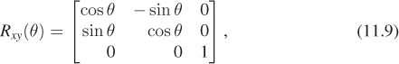
which is the rotation by angle θ in the xy-plane of 3-space. As we mentioned in Chapter 10, this is also sometimes called rotation about z by the angle θ. The advantage of calling it rotation in the xy-plane is that there is an easy mnemonic associated to it: For small values of θ, the unit vector in the x-direction is rotated toward the unit vector in the y-direction. Corresponding statements are true of Ryz and Rzx, which are written below. There’s another advantage: While rotations in 3-space always have an axis (see the web material for a proof) those in 2-space do not (e.g., there’s no vector in R2 left invariant by rotation through 30°), and neither do those in 4-space. But in all cases rotations can be described in terms of planes of rotation.
The analogous rotations in the yz- and zx-planes are given by
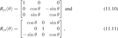
which can also be called rotation about x and rotation about y, respectively.
In contrast to the two-dimensional situation, where we found that the set of 3 × 3 rotation matrices was one-dimensional, in three dimensions the set SO(3) of 3 × 3 rotation matrices is three-dimensional. It is not, however, just a three-dimensional Euclidean space. One way to see it’s three-dimensional is to find a mostly one-to-one mapping from an easy-to-understand three-dimensional object to SO(3) (just as the latitude-longitude parameterization of the 2-sphere shows us that the 2-sphere is two-dimensional). We’ll actually describe three such mappings, each with its own advantages and disadvantages. The first of these mappings is through Euler angles. This mapping is “mostly one-to-one,” in much the same way that the mapping of latitude and longitude to points on the globe is mostly one-to-one: Each point on the international date line has two longitudes (180E and 180W), and each pole has infinitely many longitudes, but each other sphere point corresponds to a single latitude-longitude pair.
11.2.2. Euler Angles
Euler angles are a mechanism for creating a rotation through a sequence of three simpler rotations (called roll, pitch, and yaw). This decomposition into three simpler rotations can be done in several ways (yaw first, roll first, etc.); unfortunately, just about every possible way is used in some discipline. You’ll need to get used to the idea that there’s no single correct definition of Euler angles.
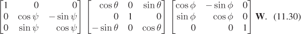
The most commonly used definition in graphics describes a rotation by Euler angles (φ, θ, ψ) as a product of three rotations. The matrix M for the rotation is therefore a product of three others:
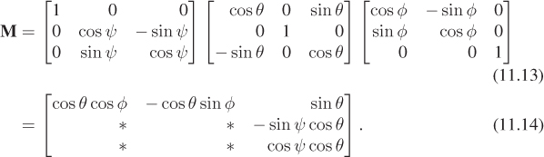
Thus, objects are first rotated by angle φ in the xy-plane, then by angle θ in the zx-plane, and then by angle ψ in the yz-plane. The number φ is called pitch, θ is called yaw, and ψ is called roll. If you imagine yourself flying in an airplane (see Figure 11.1) along the x-axis (with the y-axis pointing upward) there are three direction changes you can make: Turning left or right is called yawing, pointing up or down is called pitching, and rotating about the direction of travel is called rolling. These three are independent in the sense that you can apply any one without the others. You can, of course, also apply them in sequence.
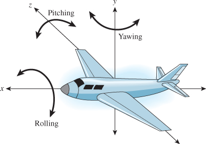
Figure 11.1: An airplane that flies along the x-axis can change direction by turning to the left or right (yawing), pointing up or down (pitching), or simply spinning about its axis (rolling).
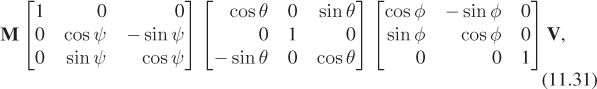
Writing this out in matrices, we have
With the proper choice of φ, θ, and ψ, such products represent all possible rotations. To see this, we’ll show how to find φ, θ, and ψ from a rotation matrix M. In other words, having shown how to convert a (φ, θ, ψ) triple to a matrix, we’ll show how to convert a matrix M to a triple (φ′, θ′, ψ′), a triple with the property that if we convert it to a matrix, we’ll get M.
The (1, 3) entry of M, according to Equation 11.14, must be sin θ, so θ is just the arcsine of this entry; the number thus computed will have a non-negative cosine. When cos θ ≠ = 0, the (1, 1) and (1, 2) entries of M are positive multiples of cos φ and – sin φ by the same multiplier; that means φ = atan2(–m12, m11). We can similarly compute ψ from the last entries in the second and third rows. In the case where cos θ = 0, the angles φ and ψ are not unique (much as the longitude of the North Pole is not unique). But if we pick φ = 0, we can use the lower-left corner and atan2 to compute a value for ψ. The code is given in Listing 11.1, where we are assuming the existence of a 3 × 3 matrix class, Mat33, which uses zero-based indexing. The angles returned are in radians, not degrees.
Listing 11.1: Code to convert a rotation matrix to a set of Euler angles.
1 void EulerFromRot(Mat33 m, out double psi,
2 out double theta,
3 out double phi)
4 {
5 theta = Math.asin(m[0,2]) //using C# 0-based indexing!
6 double costheta = Math.cos(th);
7 if (Math.abs(costheta) == 0){
8 phi = 0;
9 psi = Math.atan2(m[2,1], m[1,1]);
10 }
11 else
12 {
13 phi = atan2(-m[0,1], m[0,0]);
14 psi = atan2(-m[1,2], m[2,2]);
15 }
16 }
It remains to verify that the values of θ, φ, and ψ determined produce matrices which, when multiplied together, really do produce the given rotation matrix M, but this is a straightforward computation.
Write a short program that creates a rotation matrix from Rodrigues’ formula (Equation 11.17 below) and computes from it the three Euler angles. Then use Equation 11.14 to build a matrix from these three angles, and confirm that it is, in fact, your original matrix. Use a random unit direction vector and rotation amount in Rodrigues’ formula.
Aside from the special case where cos θ = 0 in the code above, we have a one-to-one mapping from rotations to (θ, φ, ψ) triples with –π/2 < θ ≤ π/2 and –π < φ, ψ ≤ π. Thus, the set of rotations in 3-space is three-dimensional.
In general, you can imagine controlling the attitude of an object by specifying a rotation using θ, φ, and ψ. If you change any one of them, the rotation matrix changes a little, so you have a way of maneuvering around in SO(3). The cos θ = 0 situation is tricky, though. If θ = π/2, for instance, we find that multiple (φ, ψ) pairs give the same result; varying φ and ψ turns out to not produce independent changes in the attitude of the object. This phenomenon, in various forms, is called gimbal lock, and is one reason that Euler angles are not considered an ideal way to characterize rotations.
11.2.3. Axis-Angle Description of a Rotation
One way to rotate 3-space is to pick a particular axis (i.e., a unit vector) and rotate about that direction by some amount. The matrix Rxy does this when the axis is the z-axis, for instance. We show, in the web materials, that every rotation in 3-space is rotation about some axis by some angle. Rodrigues [Rod16] discovered a formula to build a rotation for any axis and angle of rotation, and thus to produce any rotation matrix. We let
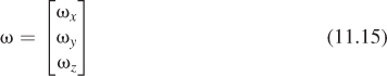
denote the unit-vector axis of rotation and θ the amount of rotation about ω (measured counterclockwise as viewed from the tip of ω looking toward the origin).
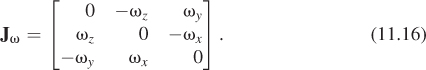
To express the rotation we seek, we’ll need to use cross products a good deal. The function v ![]() ω×v is a linear transformation from R3 to itself; the matrix for this transformation is
ω×v is a linear transformation from R3 to itself; the matrix for this transformation is
(a) What’s ω×ω?
(b) Show that Jωω = 0 as expected.
(c) Suppose that v is a unit vector perpendicular to ω. Explain why ω×v is perpendicular to both, and why ω×(ω×v) = –v.
The rotation matrix we seek is then
From Inline Exercise 11.4, it’s clear that Mω = ω. And if v is perpendicular to ω, then
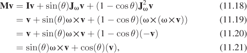
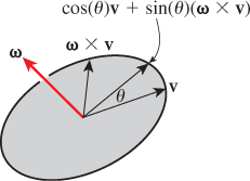
which is just the rotation of v in the plane perpendicular to ω by an angle θ. Since M does the right thing to ω and to vectors perpendicular to ω, it must be the right matrix, as per the Transformation Uniqueness principle (see Figure 11.2).
In coordinate form, it’s
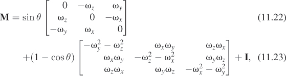
where we’ve used the fact that ω is a unit vector to simplify things a little. But the earlier form is far easier to program correctly.
11.2.4. Finding an Axis and Angle from a Rotation Matrix
As we said earlier, it’s a theorem that every rotation of 3-space has an axis (i.e., a vector that it leaves untouched). We can use Rodrigues’ formula to recover the axis from the matrix. We’ll follow the approach of Palais and Palais [PP07].
We know every rotation matrix has an axis ω and an amount of rotation, θ, about ω; Rodrigues’ formula tells us the matrix must be
for some unit vector ω and some angle θ.
The trace of this matrix (the sum of the diagonal entries) is
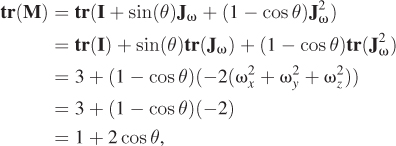
so we can recover the angle of rotation by computing
Two special cases arise at this point, corresponding to the two ways that sin θ can be zero.
1. If θ = 0, then any unit vector serves as an “axis” for the rotation, because the rotation is the identity matrix.
2. If θ = π, then twice the rotation has angle 2π, and thus is the identity, that is, our rotation M must satisfy M2 = I. From this we find that
That means that when we multiply M by M + I, every column of M + I remains unchanged. So any nonzero column of M + I, when normalized, can serve as the axis of rotation. We know that at least one column of M + I is nonzero; otherwise, M = –I. But this is impossible, because the determinant of –I is –1, while that of M is +1.
In the general case, when sin θ ≠ 0, we can compute M – MT to get
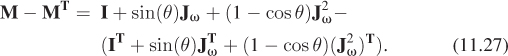
Because JTω = –Jω and (J2ω)T = J2ω, this simplifies to
Dividing by 2 sin θ gives the matrix Jω, from which we can recover ω. The code is given in Listing 11.2.
Listing 11.2: Code to find the axis and angle from a rotation matrix.
1 void RotationToAxisAngle(
2 Mat33 m,
3 out Vector3D omega,
4 out double theta)
5 {
6 // convert a 3x3 rotation matrix m to an axis-angle representation
7
8 theta = Math.acos( (m.trace()-1)/2);
9 if (θ is near zero)
10 {
11 omega = Vector3D(1,0,0); // any vector works
12 return;
13 }
14 if (θ is near π)
15 {
16 int col = column with largest entry of m in absolute value;
17 omega = Vector3D(m[0, col], m[1, col], m[2, col]);
18 return;
19 }
20 else
21 {
22 mat 33 s = m - m.transpose();
23 double x = -s[1,2], y = s[0,2]; z = s[1,1];
24 double t = 2 * Math.Sin(theta);
25 omega = Vector3D(x/t, y/t, z/t);
26 return;
27 }
28 }
A few observations are in order.
• For small θ, M is nearly the identity.
• For small θ, the coefficient of the middle term is approximately θ, while the coefficient of the last term is ![]() ; thus, the last term is far smaller than the middle term. So to first order, M ≈ I + sin θJω.
; thus, the last term is far smaller than the middle term. So to first order, M ≈ I + sin θJω.
11.2.5. Body-Centered Euler Angles
Suppose we have a model of an airplane whose vertices are stored in an 3 × n array V. We’ve rotated the model to some position that we like by multiplying all the vertices by some rotation matrix M, that is, we’ve computed
We now decide that we’d like to have the airplane model pitch up a little more (as if the pilot had pulled on the joystick). We could apply some Euler-angle rotations to the rotated vertices, that is, we could compute
The problem is that this would take the already rotated vertices and rotate them first about the world z-axis, which might point diagonally through the airplane, and then about the world y-axis, and then about the world x-axis. It would be very hard to choose ψ, θ, and φ to have the effect we are seeking. Such a transformation would be called a world-centered rotation, because the description of the rotation is in terms of the axes of the world coordinate system. We could instead compute
that is, apply some rotations to the object’s vertices before applying the rotation M to the object. Such an operation is called a body-centered rotation or object-centered rotation. In this case, performing the rotation we seek is easy: We simply adjust the pitch angle φ. Of course, if we then want to adjust it further, we have to apply another body-centered rotation, and it appears that we’re destined to accumulate a huge sequence of matrices. One solution is to explicitly compute the product so that we always have at most one matrix, plus three others temporarily being adjusted until they too can be folded into the matrix. Another approach is to represent matrices with quaternions, as we’ll see below. In general, if M is the current transformation applied to the vertex set V, and we alter it to M1 = MA, then A is called a body-centered operation, while if we alter it to M2 = CM, then C is called a world-centered operation.
11.2.6. Rotations and the 3-Sphere
The set SO(3) of all 3 × 3 rotation matrices can be difficult to understand. It is, in some sense, a subset of R9: Just read the nine entries of the matrix M in order to get the point in R9 that corresponds to M. In a web extra, we give considerable detail on this set and its properties. Here, we’ll give just the essentials. The main tool used to understand SO(3), to make computations involving SO(3) more numerically robust, and to let us reason about operations in SO(3) (like interpolation) by means of a familiar space, is S3, the 3-sphere, or the set of all points [w x y z]T in 4-space whose distance from the origin is 1. We’ve shuffled the coordinates on purpose to make some of what we say below involve less shuffling. We’ll also, in this section, talk about points of S3, but we’ll always write them as vectors so that we can form linear combinations of them.
Just as you can wrap a line segment into a circle (joining the two boundary points into one point of the circle, as in Figure 11.3), or wrap a disk into a sphere (with the whole boundary circle becoming one point of the sphere, as in Figure 11.4), you can wrap a solid ball in 3-space into a 3-sphere, by collapsing the whole boundary sphere to a point. To do so, you must work in the fourth dimension, but the idea is to reason about the 3-sphere by analogy.
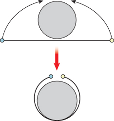
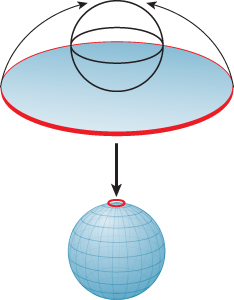
Figure 11.4: Wrapping a disk onto a sphere; all points of the circular edge of the disk are sent to the North Pole.
For instance, if we take two perpendicular unit vectors u and v in the unit circle and construct all points of the form cos(θ)u + sin(θ)v, these points cover the whole circle (see Figure 11.5). Similarly, in the 2-sphere, if we have two perpendicular unit vectors, their cosine-sine combinations form a great circle, that is, the intersection of the sphere with a plane through its center (see Figure 11.6). In fact, the same thing is true for the 3-sphere as well: Cosine-sine combinations of perpendicular vectors traverse a great circle on the 3-sphere. And the arc of this circle from u to v (i.e, from θ = 0 to π/2) is the shortest path between them, just as in the lower dimensions.
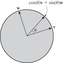
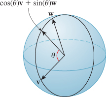
Figure 11.6: All cosine-sine combinations of two perpendicular unit vectors in the sphere again form a unit circle, called a great circle.
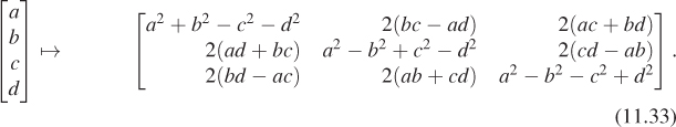
There’s a mapping from S3 to SO(3), given by
The map K has several nice properties.
• It’s almost one-to-one. In fact, it’s a two-to-one map; for any q ![]() S3, K(q) = K(–q), as you can see by looking at the formula.
S3, K(q) = K(–q), as you can see by looking at the formula.
• Great circles on S3 are sent, by K, to geodesics (paths of shortest length) in SO(3).
• K([1 0 0 0]T) = I.
This mapping arises from a definition of a kind of “multiplication” on R4, closely analogous to the way we can treat points of R2 as complex numbers and multiply them together. The multiplication on R4 is not commutative, which causes some difficulties, but otherwise it’s closely analogous to multiplication of complex numbers. The set R4, together with this multiplication operation, is called the quaternions (which is why we use a boldface q for a typical element of S3). The web material for this chapter describes the quaternions in detail, derives the mapping K above, and shows how it’s related to Rodrigues’ formula. For most purposes in graphics, it’s sufficient to know the three properties above, and one more fact, which we now develop.
If we have a point q = [a b c d]T ![]() S3, we know –1 ≤ a ≤ 1, so a is the cosine of some number. We let
S3, we know –1 ≤ a ≤ 1, so a is the cosine of some number. We let
Furthermore, since [a b c d]T ![]() S3, we know that a2 + b2 + c2 + d2 = 1. Thus,
S3, we know that a2 + b2 + c2 + d2 = 1. Thus,
so that [b c d]T is a vector of squared length sin2(θ). If a ≠ ±1, then sin(θ) ≠ 0, and we can let
and say that
In the case where sin(θ) = 0, we can choose any unit vector for ω. In short, every element of S3 can be written in the form
where 0 ≤ θ ≤ π and ω is a unit vector in the xyz-subspace of S3, that is, perpendicular to [1 0 0 0]T.
With a good deal of algebra, you can plug in a = cos(θ), b = sin(θ)ωx, c = sin(θ)ωy, and d = sin(θ)ωz in Equation 11.32, and discover that it’s exactly the same matrix you get if you apply Rodrigues’ formula to build a rotation about the xyz-vector ω by angle 2θ (note the factor of two!).
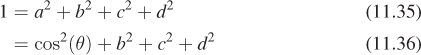
The map K has a great deal in common with the map K1 : S1 ![]() S1 : (cos(θ), sin(θ))
S1 : (cos(θ), sin(θ)) ![]() (cos(2θ), sin(2θ)). Like K, the map K1 is also two-to-one. For instance, the points at θ = 0 and θ = π both get sent to the point at θ = 0 by K1. In fact, the points at θ and θ + π are both sent to the point at θ, for any angle θ; in other words, K1 maps each pair of antipodal points to the same point. If you wanted to interpolate between, say, π/4 and 3π/4 in the codomain, you could pick the points π/8 and 3π/8 in the domain, interpolate between them, and then apply K1 to the interpolated angles and get the result you expect. Of course, if instead of picking 3π/8, you pick 11π/8, then the interpolation will run along the long path between π/4 and 3π/4, as shown in Figure 11.7.
(cos(2θ), sin(2θ)). Like K, the map K1 is also two-to-one. For instance, the points at θ = 0 and θ = π both get sent to the point at θ = 0 by K1. In fact, the points at θ and θ + π are both sent to the point at θ, for any angle θ; in other words, K1 maps each pair of antipodal points to the same point. If you wanted to interpolate between, say, π/4 and 3π/4 in the codomain, you could pick the points π/8 and 3π/8 in the domain, interpolate between them, and then apply K1 to the interpolated angles and get the result you expect. Of course, if instead of picking 3π/8, you pick 11π/8, then the interpolation will run along the long path between π/4 and 3π/4, as shown in Figure 11.7.
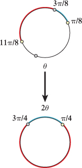
Figure 11.7: The blue path in the domain transforms to the short arc between π/4 and 3π/4 in the codomain, while the red one transforms to the long arc.
By the way, although K is not invertible, it’s easy to build a kind of inverse: Given M ![]() SO(3), we can find an element q
SO(3), we can find an element q ![]() S3 with K(q) = M; we just cannot claim that it is the element with this property. Recall that Rodrigues’ formula tells us that every rotation matrix has the form
S3 with K(q) = M; we just cannot claim that it is the element with this property. Recall that Rodrigues’ formula tells us that every rotation matrix has the form
where ω is a unit vector that’s the axis of rotation of the matrix and θ is the angle of rotation. And we discussed how to recover the axis ω and the angle θ from an arbitrary rotation matrix (except that when the matrix was I, the axis could be any unit vector and the angle was 0). The associated element q of S3 has cos(θ/2) as its first coordinate and sin(θ/2)ω as its last three coordinates. The case where θ = 0 and ω is indeterminate presents no problem, because sin(θ/2) = 0, so the last three entries are all zeroes. There is an ambiguity, however: When we found the axis ω and the angle θ we could instead have found –ω and –θ; those two would have produced –q instead of q. So our “inverse” to K really can produce one of two opposite values, depending on choices made in the axis-and-angle computation. To make all this concrete, we’ll give pseudocode for a function L whose domain is SO(3) and whose codomain is pairs of antipodal points in S3; L will act as an inverse to K, in the sense that if M ![]() SO(3) is a rotation matrix and L(M) = {q1, – q1} are two elements of S3, then K(q1) = K(–q1) = M. In the pseudocode in Listing 11.3, neither
SO(3) is a rotation matrix and L(M) = {q1, – q1} are two elements of S3, then K(q1) = K(–q1) = M. In the pseudocode in Listing 11.3, neither q1 nor q2 is guaranteed to be a continuous function of the entries of the matrix m.
Listing 11.3: Code to convert a rotation matrix to the two corresponding quaternions.
1 void RotationToQuaternion(Mat33 m, out Quaternion q1, out Quaternion q2)
2 {
3 // convert a 3x3 rotation matrix m to the two quaternions
4 // q1 and q2 that project to m under the map K.
5 if (m is the identity)
6 {
7 q1 = Quaternion(1,0,0,0);
8 q2 = -q1;
9 return;
10 }
11
12 Vector3D omega;
13 double theta;
14 RotationToAxisAngle(m, omega, theta);
15
16 q1 = Quaternion(Math.cos(theta/2), Math.sin(theta/2)*omega);
17 q2 = -q1;
18 }
We now have a method for going from S3 to SO(3) and for going from SO(3) back to pairs of elements of S3. To interpolate between rotations in SO(3), we’ll interpolate between points of S3.
11.2.6.1. Spherical Linear Interpolation
Suppose we have two points q1 and q2 of the unit sphere, and that q1 ≠ –q2, that is, they’re not antipodal. Then there’s a unique shortest path between them, just as on the Earth there’s a unique shortest path from the North Pole to any point except the South Pole. (There is a shortest path from the North to the South Pole; the problem is that it’s no longer unique—any line of longitude is a shortest path.)
We’ll now construct a path γ that starts at q1 (i.e., γ(0) = q1), ends at q2 (i.e., γ(1) = q2), and goes at constant speed along the shorter great arc between them. This is called spherical linear interpolation and was first described for use in computer graphics by Shoemake [Sho85], who called it slerp. There are three steps.
1. Find a vector v ![]() S3 that’s in the q1–q2 plane and is perpendicular to q1. We subtract the projection (q2 · q1)q1 of q2 onto q1 from q2 to get a vector perpendicular to q1, and normalize:
S3 that’s in the q1–q2 plane and is perpendicular to q1. We subtract the projection (q2 · q1)q1 of q2 onto q1 from q2 to get a vector perpendicular to q1, and normalize:
2. Find a unit-speed path along the great circle from q1 through v. That’s just γ(t) = cos(t)q1 + sin(t)v. This path reaches q2 at t = θ, where θ = cos–1(q1 · q2) is the angle between the two vectors.
3. Adjust the path so that it reaches q2 at time 1 rather than at time θ, by multiplying t by θ.
The resultant code is shown in Listing 11.4.
Listing 11.4: Code for spherical linear interpolation between two quaternions.
1 double[4] slerp(double[4] q1, double[4] q2, double t)
2 {
3 assert(dot(q1, q1) == 1);
4 assert(dot(q2, q2) == 1);
5 // build a vector in q1-q2 plane that’s perp. to q1
6 double[4] u = q2 - dot(q1, q2) * q2;
7 u = u / length(u); // ...and make it a unit vector.
8 double angle = acos(dot(q1, q2));
9 return cos(t * angle) * q1 + sin(t * angle) * u;
10 }
As the argument to the cosine ranges from 0 to angle, the result varies from q1 to q2.
11.2.6.2. Interpolating between Rotations
We now have all the tools we need to interpolate between rotations. Suppose that M1 and M2 are rotation matrices, with M1 corresponding to the quaternions ±q1 and M2 corresponding to the quaternions ±q2, as indicated schematically in Figure 11.8. Starting with q1, we determine which of q2 and –q2 is closer, and then interpolate along an arc between q1 and this point; to find interpolating rotations, we project to SO(3) via K.

Figure 11.8: We have two rotation matrices, M1 and M2; the first corresponds to a pair of antipodal quaternions, ±q1, and the second to a different pair of antipodal quaternions, ±q2. Starting at q1, we choose whichever of q2 and –q2 is closer (in this case, –q2) and interpolate between them (as indicated by the thick red arc); we then can project the interpolated points to SO(3) to interpolate between M1 and M2.
Listing 11.5 shows the pseudocode.
Listing 11.5: Code to interpolate between two rotations expressed as matrices.
1 Mat33 RotInterp(Mat33 m1, Mat33 m2, double t)
2 // find a rotation that’s t of the way from m1 to m2 in SO(3).
3 // m1 and m2 must be rotation matrices.
4 {
5 if (![]() ){
){
6 Report error; can’t interpolate between opposite rotations.
7 }
8 Quaternion q1, q1p, q2, q2p;
9 RotationToQuaternion(m1, q1, q1p);
10 RotationToQuaternion(m2, q2, q2p);
11 if (Dot(q1, q2) < 0) q2 = q2p;
12 Quaternion qi = Quaternion.slerp(q1, q2, t);
13 return K(qi); // K is the projection from S3 to SO(3)
14 }
With this notion of “interpolate between rotations” or “interpolate between quaternions” in hand, other operations, like blending together three or four rotations, also become possible. Indeed, even operations like the curve subdivision we did in Chapter 4 become possible in SO(3) instead of R2. One must be careful, however. While it’s nice to be able to interpolate between quaternions in the same way we construct a segment between points in the plane, the analogy has some weaknesses: In the plane, we can construct points (1 – t)A + tB for t between 0 and 1, and they lie between A and B. If we use t > 1, we get a point “beyond B.” On the other hand, if we do spherical linear interpolation between quaternions q1 and q2, as we increase t further and further, the result eventually wraps around the sphere and returns to q1.
Other “obvious” things fail as well. In the plane, we can find the center of a quadrilateral by bisecting opposite sides and finding the midpoint of the edge between these points. It doesn’t matter which pair of opposite sides we choose—the result is the same, as shown in Figure 11.9. But with quaternions, it’s generally not the same.
Figure 11.9: We can compute the midpoint of the quadrilateral ABCD by finding the midpoints of AB and CD (marked by circles), and then the midpoint of the segment between them, or by doing the same process to the edges AD and BC (whose midpoints are marked by squares); the resultant quadrilateral midpoint (indicated by the diamond) is the same in both cases. This does not happen when we work with quaternions.
On the 2-sphere, let A = B = (0, 1, 0), C = (1, 0, 0), and D = (0, 0, 1). Compute (by drawing—you should not need to perform any algebra) the center of the quadrilateral ABCD twice, once using each pair of opposite sides, to verify that the results are not the same.
Buss [BF01] discusses thoroughly the challenges of working with such “affine combinations” of quaternions.
11.2.7. Stability of Computations
You probably recall solving problems in calculus where you know a position x(t) at time t = 0, and you’re given a formula for velocity x′ (t) for all t, and you need to find x at times other than t = 0. The simple method is to say that at t = 0.1, your position is approximately
and then compute x(0.2) ≈ x(0.1) + 0.1x′ (0.1), etc. This is called Euler integration of the position with a time step of 0.1, and it gives a crude approximation of the solution to the problem. Picking a time step smaller than 0.1 produces better results, but at a cost of greater computational effort. Chapter 35 discusses this, and better approximations, extensively.
The analogy for the attitude (i.e., the rotation matrix currently applied to some model) is that you’re given the attitude at time t = 0, and the change in attitude for all t, and you have to “integrate” to find the attitude at all times. The “update” step is
so that it’s multiplicative rather than additive. One problem is that I + 0.1M′ (0) is not actually a rotation matrix. It’s very close, but not quite. So, after the update, we have to convert M into a rotation matrix, typically by applying the Gram-Schmidt process to the columns of M (i.e., normalize the first column; make the second perpendicular to it; normalize the second; make the third perpendicular to both; normalize the third column). This is computationally fairly expensive.
As an alternative, we can store the current attitude as a unit quaternion q. The update, in that case, looks like this:
Once again, the resultant vector at t = 0.1 is not quite what we want: It may not be a unit vector, so we have to normalize it. Notice, however, that normalizing a vector requires much less work than performing the Gram-Schmidt process on a whole matrix. And while a matrix can fail to be a rotation in many ways (one or more columns not unit length, various pairs of columns not perpendicular), a quaternion can fail to be a unit quaternion in only one way. For this reason, animation systems often represent attitude with a quaternion, converting it to a rotation matrix with the map K only when necessary. Computations on a quaternion tend to be more numerically stable than those on a rotation matrix as well.
11.3. Comparing Representations
We’ve now seen four ways to represent a 3D rigid reference frame (i.e., a set of three orthogonal unit vectors forming a right-handed coordinate system, based at some location P).
1. A 4 × 4 matrix M, which we apply to the standard basis vectors at the origin to get the three vectors, and to the origin itself to get the basepoint P. The last row of the matrix must be [0 0 0 1], and the upper-left 3 × 3 submatrix S must be a rotation matrix.
2. A 3 × 3 rotation matrix S and a translation vector t = P – origin.
3. Three Euler angles and a translation vector.
4. A unit quaternion and a translation vector.
Each has its advantages.
Option 1 is nice because it’s easy to consider it as a transformation, which can be combined with other transformations by matrix multiplication. It makes sense to use this in a geometric modeling system. Converting between options 1 and 2 is straightforward, but option 2 has the advantage that it’s easy to check that the matrix S is orthogonal by checking STS = I. If several such matrices have been multiplied, accumulating round-off errors, you can apply the Gram-Schmidt orthogonalization process to the result to adjust it back into orthogonal form, although this involves many multiplications and divisions, and several square roots.
Option 3 is useful, especially in a body-centered form, for representing things like aircraft or other first-person-control situations. Converting to and from matrix form is somewhat messy, however.
Option 4 is much favored in rigid-body animation. Converting to matrix form is easy; converting from matrix form is slightly messier because of the two-to-one nature of the quaternion-to-rotation map. Interpolation is particularly easy in quaternion form, and the equivalent of “reorthogonalization” in the matrix form is vector normalization for the quaternion, which is very fast. This is discussed further in Section 35.5.2.
11.4. Rotations versus Rotation Specifications
We’ve defined a rotation as a transformation having certain properties; in particular, it’s a linear function from R3 to R3 represented by multiplication by some matrix. Thus, for instance, the transformation represented by multiplication by
can be called rotation about the z-axis (or in the xy-plane) by 90°. But it’s important to understand that multiplying a vector v by this matrix doesn’t rotate v about the z-axis in the sense that this phrase is commonly used. The vector v is at no point rotated by 10°, or 20°, or 30°. The function simply takes the coordinates of v and returns the coordinates of the rotated-by-90° version of v. Indeed, looking at the coordinates returned by the rotation, there’s no way to tell whether they arose as the result of rotation by 90°, –270°, or 450°. This might seem irrelevant in the sense that we got the rotation we wanted, but when we consider the problem of interpolating rotations it’s really quite significant. If we attempt to build an interpolation procedure interp(M1, M2, t) that takes as input two matrices M1 and M2 and a fraction t by which to interpolate them, what should happen when M1 arises from the operation “rotate not at all” and so does M2? Obviously, the interpolated rotation will not rotate at all (i.e., it’ll be the identity rotation). But what if M1 comes from “rotate not at all” and M2 comes from “rotate 360° about the z-axis”? We know that we want the halfway interpolation (t = 0. 5) to be “rotate 180° about the z-axis,” but there’s no way for our procedure to compute this: In both our cases, the matrices M1 and M2 are the identity!
In many situations, the underlying desire is not to interpolate rotation matrices or rotation transformations, but to interpolate the rotation specifications and then compute the transformation associated to the interpolated specification. Unfortunately, interpolating specifications is not so easy. In the case of axis-angle specifications, it’s easy when the axis doesn’t change: One simply interpolates the angle. But interpolating the axis is a trickier matter. And suppose we consider two instances of the problem.
1. Rotation 1: Rotate by 0 about the x-axis. Rotation 2: Rotate by 90° about the x-axis.
2. Rotation 1: Rotate by 0 about the y-axis. Rotation 2: Rotate by 90° about the x-axis.
Should the halfway interpolated rotation in these two cases be the same or different? The initial and final rotations are identical in the two cases. The only difference is in the specification of the irrelevant direction in the no-angle rotation. Should that make a difference?
Yahia and Gagalowicz [YG89] describe a method for axis-angle interpolation in which the axis always has an effect, even when the angle is a multiple of 2π; aside from this artifact, the method is quite reasonable.
11.5. Interpolating Matrix Transformations
Despite the claim of the preceding section that, in general, we want to interpolate rotation specifications rather than the transformations themselves, there are several circumstances in which directly acting on the transformations makes sense. For instance, if we’ve written a physics simulator that computes the orientations and positions of bodies at certain times, but we’d like to fill in orientations and positions at intermediate times, we can ensure that the values provided at the key times by the simulator will be fairly close to the neighboring values (i.e., an object isn’t going to spin 720° between key times) by working with small enough time steps. Given two such “nearby” transformations, can we interpolate between them?
Alexa et al. [Ale02] describe a method for interpolating transformations and more generally for forming linear combinations of transformations, provided that the transformations being combined are “near enough.” The web material for this chapter describes this method, but since it involves the matrix exponential and other mathematical topics we don’t wish to delve into, we omit it here.
11.6. Virtual Trackball and Arcball
As an application of our study of the space of rotations, we’ll now examine two methods for controlling the attitude of a 3D object that we’re viewing. These two user-interface techniques are really a part of the general topic of 3D interaction (see Chapter 21, where we give actual implementations), but we discuss them here because they are so closely related to the study of SO(3).
Our standard 3D test program can display geometric objects modeled as meshes. Imagine that we have a fixed mesh K with vertices P0, P1, ..., Pk. We can, before displaying the mesh K, apply a transformation to each of the points Pi to create a new mesh. By displaying this new mesh, we see a transformed version of K. If we repeatedly vary the transformation applied to the mesh K, we’ll see a sequence of new meshes that appears to move over time.
An alternative view of this is that we leave the mesh K fixed, but repeatedly change our virtual camera’s position and orientation. We’ll take the first approach here, however. Not surprisingly, the two are closely related: Moving the object in one direction is equivalent to moving the virtual camera in the opposite direction, for instance (as long as there’s only one object in the world).
Suppose we want to be able to view the object from all sides. We’ll assume that it’s positioned at the origin so that applying rotations to it keeps it in the same location, but with a varying attitude. How can we control the viewing direction?
One easy-to-understand metaphor is to imagine the object as being encased in a large spherical block of glass (see Figure 11.10). This glass ball is so large that if it were drawn on the display, it would fill up as much of the display as possible. (For a square display, it would touch all four sides of the display.) We can now imagine interacting with this virtual sphere by clicking on some point of the sphere, dragging some distance, and releasing. If we click first at a point P and release at the point Q, this is supposed to rotate the sphere so as to make the point P move to the point Q along a great-circle arc (i.e., to rotate in the plane defined by P, Q, and the origin).
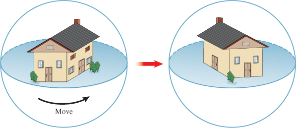
Figure 11.10: The object being viewed is imagined as lying in a large glass sphere. Moving a point on the surface of the sphere moves the object inside.
Of course, when we click on a point of the display with the mouse cursor we’re not actually clicking on the sphere—what we get are the coordinates of the point on the display surface. This in turn must be used to determine a point of the sphere itself. Suppose, for now, that we know the position C of the virtual camera, and that in response to a mouse-click, we are given the position of a corresponding point S on a plane in 3-space that corresponds to our display (see Figure 11.11).
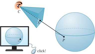
Figure 11.11: When the user clicks near the lower-right corner of the display, we can recover the 3-space coordinates of a corresponding point S of the imaging plane in 3-space; we’ll use this to determine where a ray from the eye through this point hits the virtual sphere.
To determine the point P corresponding to this click, we ask where the ray parameterized by
meets the virtual sphere, which we’ll assume, for simplicity, is the unit sphere defined by x2 + y2 + z2 = 1. In other words, the unit sphere, if displayed, would just touch two sides of our display rectangle. For the point R(t) to lie on the sphere, its coordinates (which we’ll call rx, ry, and rz) must satisfy the defining equation of the sphere, that is,
Alternatively, we can consider the vector from the origin O to R(t), that is, C + t(S – C) – O; this vector must have unit length, which means it must satisfy (R(t) – O) · (R(t) – O) = 1. Letting u denote S – C, this becomes
which we can simplify and expand; letting c = C – O, we get
which is a quadratic in t; we solve to get
The smaller t value—call it t1—corresponds to the first intersection of the ray with the sphere; using this, we can compute the sphere point
(It’s possible that both solutions for t are not real numbers, in which case the ray does not intersect the sphere: The user did not click on the image of the virtual sphere on the display.)
As the user drags the mouse, we can, at each instant, compute the corresponding sphere point Q in the same way. From P and Q, we compute a rotation of the sphere that takes P to Q along a great circle; this rotation must be about a unit vector orthogonal to P and Q, and it must have magnitude cos–1(P · Q). Rodrigues’ formula provides the matrix.
We use this matrix to multiply all vertex coordinates of the original mesh to get a new mesh for display; the resultant operation feels completely natural to many people.
Two problems remain: What happens when the user drags to a point outside the virtual sphere? And what happens when the user’s initial click is outside the virtual sphere?
Various solutions have been implemented. When the user drags outside the virtual sphere, one good solution is to treat the point Q as being the nearest point on the sphere to the ray that the user is describing; this corresponds to using t = – c · u/u · u in the quadratic solution.
When the user clicks outside the virtual sphere, one can treat subsequent mouse-drags as instructions to rotate about the view direction, like the “rotate object” interaction in most 2D drawing programs.
One problem with the virtual-sphere controller described so far is that the action of the controller depends on the first point the user clicked; in a long interaction sequence, this may be gradually forgotten. An improved approach is to treat each mouse-drag event as defining a new motion of the sphere, taking the start point to the endpoint. Thus, a click and drag becomes a sequence of mouse positions P0 = P, P1, P2, ..., Pn = Q, and the object is rotated by a sequence of virtual-sphere rotations from P0 to P1, followed by the rotation defined by P1 and P2, etc.
With this modified version of the virtual sphere, it can be difficult to return to one’s starting position; in trade for this, one gets the advantage that a click-and-drag-in-small-circles motion causes the object to spin about the view direction, which users seem to learn instinctively.
There’s a different approach to virtual-sphere rotation developed by Shoemake [Sho92], in which a click and drag from P to Q rotates the sphere from P toward Q, but by double the angle used in the virtual sphere. A click at the center of the virtual arcball followed by a drag to the edge of the arc ball produces not a 90° rotation, but a 180° rotation. This has the advantage that one can achieve any desired rotation of the object by a single click and drag (e.g., spins about the view direction are generated by dragging from one point near the boundary of the ball to another).
11.7. Discussion and Further Reading
For the mathematically inclined, the study of SO(n) is covered in several books [Che46, Hus93, Ste99], and some of the basic properties of Sn and SO(n) are discussed in many introductory books on manifolds [GP10, Spi79a].
The classic work on quaternions is by Hamilton [Ham53], but more modern expositions [Che46, Hus93] are much easier to read.
Quaternions are an instance of a more general phenomenon developed by Grassmann [Gra47] in which noncommutative forms of multiplication played a central role. Unfortunately, Grassmann’s ideas were so confusingly expressed that they were largely ignored by his contemporaries. There has been some renewed interest in them in physics (and some related interest in graphics), with recent developments being given the name geometric algebra [HS84, DFM07].
11.8. Exercises
Exercise 11.1: We computed the matrix for reflection through the line determined by the unit vector u by reasoning about dot products. But this reflection is also identical to rotation about u by 180°. Use the axis-angle formula for rotation to derive the reflection matrix directly.
Exercise 11.2: In Rn, what is the matrix for reflection through the subspace spanned by e1, ..., ek, the first k standard basis vectors? In terms of k, tell whether this reflection is orientation-preserving or reversing.
Exercise 11.3: Write down the matrices for rotation by 90° in the xy-plane and rotation by 90° in the yz-plane. Calling these M and K, verify that MK = KM, thus establishing that in general, if R1 and R2 are elements of SO(3), it’s not true that R1R2 = R2R1; this is in sharp contrast to the set SO(2) of 2 × 2 rotation matrices, in which any two rotations commute.
Exercise 11.4: In Listing 11.2, we have a condition “if θ is near π” which handles the special case of very-large-angle rotations by picking a nonzero column v of M + I as the axis. If θ is not exactly π, then v will not quite be parallel to an axis. Explain why v + Mv will be much more nearly parallel to the axis. Adjust the code in Listing 11.2 to apply this idea repeatedly to produce a very good approximation of the axis.
Exercise 11.5: Consider the parameterization of rotations by Euler angles, with θ = π/2. Show that simultaneously increasing φ and decreasing ψ by the same amount results in no change in the rotation matrix at all.
Exercise 11.6: The second displayed matrix in Equation 11.23 is the square of the first (Jω); it’s also symmetric. This is not a coincidence. Show that the square of a skew-symmetric matrix is always symmetric.
![]() Exercise 11.7: Find the eigenvalues and all real eigenvectors for Jω. Do the same for J2ω.
Exercise 11.7: Find the eigenvalues and all real eigenvectors for Jω. Do the same for J2ω.
![]() Exercise 11.8: Suppose that A is a rotation matrix in R3.
Exercise 11.8: Suppose that A is a rotation matrix in R3.
(a) How many eigenvalues does a 3 × 3 matrix have?
(b) Show that the only real eigenvalue that a rotation matrix can have is ±1. Hint: A rotation preserves length.
(c) Recall that for a real matrix, nonreal eigenvalues come in pairs: If z is an eigenvalue, so is ![]() . Use this to conclude that A must have either one or three real eigenvalues.
. Use this to conclude that A must have either one or three real eigenvalues.
(d) Use the fact that if z is a nonzero complex number, then ![]() , and the fact that the determinant is the product of the eigenvalues to show that if A has a nonreal eigenvalue, it also has a real eigenvalue which much be 1, and that if A has only real eigenvalues, at least one of them must be 1.
, and the fact that the determinant is the product of the eigenvalues to show that if A has a nonreal eigenvalue, it also has a real eigenvalue which much be 1, and that if A has only real eigenvalues, at least one of them must be 1.
(e) Conclude that since 1 is always an eigenvalue of A, there’s always a nonzero vector v with Av = v, that is, the rotation A has an axis.
Exercise 11.9: The skew-symmetric matrix Jω associated to a vector ω is the matrix for the linear transformation v ![]() ω×v.
ω×v.
(a) Show that every 3 × 3 skew-symmetric matrix S represents the cross product with some vector ω, that is, describe an inverse to the mapping ω ![]() Jω.
Jω.
![]() (b) Now use this to explain why every 3 × 3 skew-symmetric matrix has 0 as an eigenvalue, hence det S = 0.
(b) Now use this to explain why every 3 × 3 skew-symmetric matrix has 0 as an eigenvalue, hence det S = 0.
Exercise 11.10: In the description of the virtual-sphere controller, we used the angle θ = cos– 1(P·Q), which involves a dot product of points rather than vectors. This worked only because we assumed that the center of our virtual sphere was the origin.
(a) Suppose the center was some other point B; how would we have computed θ?
(b) Now suppose that the virtual sphere was no longer assumed to be a unit sphere. How would we compute θ?
Exercise 11.11: Use the 3D test bed to implement virtual-sphere control for viewing.
Exercise 11.12: Given a point P and a direction v, describe how to build a transformation on R3 that rotates by θ about the line determined by P and v so that the plane through P, orthogonal to v, rotates counterclockwise by θ when viewed from the point P + v.
Exercise 11.13: We saw in Chapter 7 that if f is the test function for the plane containing the point Q and with normal n, that is, f (P) = (P – Q) · n, then we could compute the intersection of the ray t ![]() A + t w with this plane by writing g(t) = A + tw and solving f (g(t)) = 0. Suppose that T is a linear transformation with 4 × 4 matrix M—perhaps translation by some amount, or a rotation about the y-axis by 30°. We can imagine applying T to every point of the plane defined by f to get a new plane, and then finding the intersection of our ray with the new plane.
A + t w with this plane by writing g(t) = A + tw and solving f (g(t)) = 0. Suppose that T is a linear transformation with 4 × 4 matrix M—perhaps translation by some amount, or a rotation about the y-axis by 30°. We can imagine applying T to every point of the plane defined by f to get a new plane, and then finding the intersection of our ray with the new plane.
(a) George proposes that a test function ![]() for the new plane can be defined by
for the new plane can be defined by ![]() (P) = f (T(P)). Is he correct? If not, adjust his claim to a correct one.
(P) = f (T(P)). Is he correct? If not, adjust his claim to a correct one.
(b) Show that ![]() (g(t)) = 0 if and only if f (
(g(t)) = 0 if and only if f (![]() (t)) = 0, where
(t)) = 0, where ![]() (t) = M–1A + tM–1w.
(t) = M–1A + tM–1w.
(c) Describe how you can use the idea of part (b) to compute a ray-object intersection between a ray and an object that has been transformed by some affine transformation, assuming you know how to do ray-object intersection for some standard form of the object. This allows you, for instance, to ray-trace a stretched, rotated unit sphere (i.e., an ellipsoid) if you know only how to ray-trace the standard unit sphere.
![]() (d) Often in ray tracing it’s necessary to determine not only the intersection point, but also the normal vector at the intersection point. Suppose that instead of intersecting a ray R with a transformed sphere, you intersect an inverse-transformed version of R with the unit sphere at the origin, and find the intersection is at a point P = (x, y, z) with normal vector n = [x y z]T. How can you find the normal vector to the transformed sphere? Note: This approach to ray tracing is somewhat out of favor for complex scenes, as traversing the modeling hierarchy for every ray is a big cost. Instead, flattening the hierarchy by converting everything to triangles and using a spatial data structure to accelerate intersection testing turns out to be faster in general, but not always: In a forest of 1 million identical trees, each a copy of a single million-triangle tree, the spatial data structure approach fails. Instead, we make a spatial data structure whose leaves are bounding boxes for the individual trees, use the transforming-rays trick of this exercise, and proceed to trace each ray in the archetype tree’s modeling space, possibly using a spatial data structure there to accelerate the computation. This is another application of the Coordinate-System/Basis principle.
(d) Often in ray tracing it’s necessary to determine not only the intersection point, but also the normal vector at the intersection point. Suppose that instead of intersecting a ray R with a transformed sphere, you intersect an inverse-transformed version of R with the unit sphere at the origin, and find the intersection is at a point P = (x, y, z) with normal vector n = [x y z]T. How can you find the normal vector to the transformed sphere? Note: This approach to ray tracing is somewhat out of favor for complex scenes, as traversing the modeling hierarchy for every ray is a big cost. Instead, flattening the hierarchy by converting everything to triangles and using a spatial data structure to accelerate intersection testing turns out to be faster in general, but not always: In a forest of 1 million identical trees, each a copy of a single million-triangle tree, the spatial data structure approach fails. Instead, we make a spatial data structure whose leaves are bounding boxes for the individual trees, use the transforming-rays trick of this exercise, and proceed to trace each ray in the archetype tree’s modeling space, possibly using a spatial data structure there to accelerate the computation. This is another application of the Coordinate-System/Basis principle.