
Chapter 35. Motion
35.1. Introduction
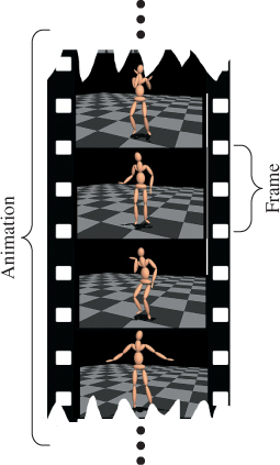
When you see a sequence of related images in rapid succession, they blend together and create the perception that objects in the images are moving. This need not involve a computer: Cartoons drawn in a flip-book and analog film projection (see Figure 35.1) both create the illusion of motion this way. The individual images are called frames and the entire sequence is called an animation. Beware that both of these terms have additional meanings in computer graphics; for example, a coordinate transform is a “reference frame” and an “animation” can refer to either the rendered images or the input data describing one object’s motion.
This chapter presents some fundamental methods for describing the motion of objects in a 3D world over time. These mainly involve either interpolating between key positions (see Figure 35.2) or simulating dynamics according to the laws of physics (see Figure 35.3). Note that the laws of physics as in a virtual world need not be those of the real world.
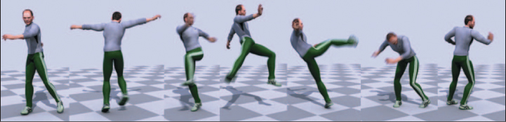
Figure 35.2: A series of key poses extracted from dense motion capture data [SYLH10] that have been visualized by rendering a virtual actor in those poses. (Courtesy of Moshe Mahler and Jessica K. Hodgins.)
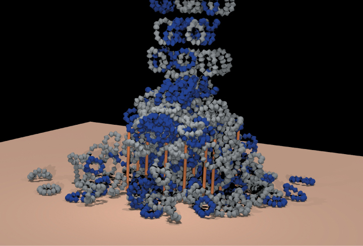
Figure 35.3: Hundreds of complex shapes fall into a pile in this rigid-body simulation of Newtonian mechanics [WTF06]. This kind of simulation is leveraged extensively to present “what if?” scenarios for both entertainment and engineering applications. The primary challenges are efficiency and numerical stability. (Courtesy of Ron Fedkiw and Rachel Weinstein Petterson, ©2005 ACM, Inc. Reprinted by permission.)
Most character animation that you have observed was driven by key positions, with those positions created either by an artist or via motion capture of an actor (see Figure 35.4). Those processes are not particularly demanding from a computational perspective, but producing the animations is expensive and relatively slow because of the time and skill that they require from the artists in the process. In contrast, dynamics is computationally challenging but requires comparatively little input from an artist. This is a classic example of leveraging a computer to multiply a human’s efforts dramatically. It is natural that as animation algorithms have become more sophisticated and computer hardware has become both more efficient and less expensive, the broad trend has been to increase the amount of animation produced by dynamics.
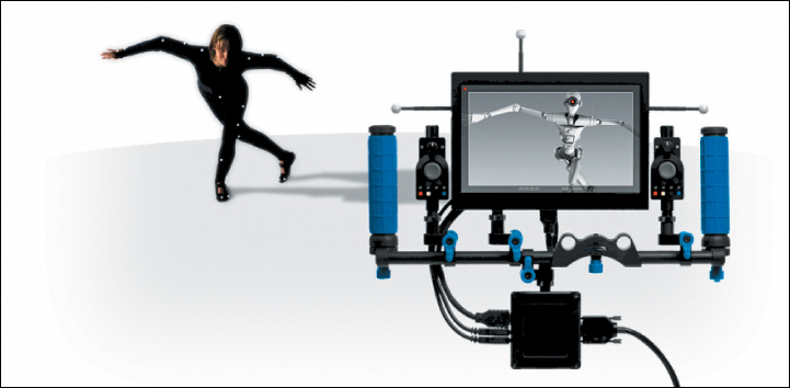
Figure 35.4: Motion capture systems, such as the InsightVCS system pictured, record the three-dimensional motion of a real actor and then apply those motions to avatars in the virtual scene. (Courtesy of OptiTrack.)
The artistry and algorithms of animations are subjects that have filled many texts, and thus even a survey would strain the bounds of a single chapter. This chapter focuses on the rendering and computational aspects of physically based animation. In particular, it emphasizes concepts in the interpolation and rendering sections and mathematical detail in the dynamics section. Dynamics is primarily concerned with numerical integration of estimated derivatives; thinking deeply about the underlying calculus should help you navigate the notorious difficulty of achieving stability and accuracy in such a system. The techniques used are related to several other numerical problems beyond physical simulation. Notably, the integration methods that arise in dynamics serve as another example of the techniques applied to the integration of probability density and radiance functions in light transport.
There are many other ways to produce animations that are not discussed in this chapter. Two popular ones are filtering live-action video (e.g., as shown in Figure 35.5) and computing per-pixel finite automata simulation (e.g., Conway’s Game of Life [Gar70], Minecraft, and various “falling sand” games). Although beyond the scope of this book, both filtering and finite automata make rewarding graphics projects that we recommend to the reader.

Figure 35.5: Video tooning creates an animation from live-action footage [WXSC04]. This kind of algorithm is an important open-research topic and a great project, but it is not discussed further in this chapter. (Courtesy of Jue Wang and Michael Cohen. Drawn and performed by Lean Joesch-Cohen. ©2004 ACM, Inc. Reprinted by permission.)
Finally, artists are essential! Even the best animation algorithms are ineffective without expressive input data, and the worst animation algorithms can succeed if controlled by a master animator. Those input data are created by artists employing animation tools that are themselves complex software. To build such tools one must appreciate the artists’ goals and approach to animation. These tools shape the format of the data that then feed the runtime systems.
35.2. Motivating Examples
We begin with ad hoc methods for creating motion in some simple scenes. These illuminate the important issues of animation and suggest methods for generalizing to more formal methods.
35.2.1. A Walking Character (Key Poses)
Consider the case of creating an animation of a person walking. Let the person be modeled as a 3D mesh represented by a vertex array and an indexed triangle list as described in Chapter 14. Assume that an artist has already created several variations on this mesh that have identical index lists but potentially different vertex positions. These mesh variations represent different poses of the character during its walk. Each one is called a key pose or key frame. The terminology dates back to hand-animated cartoons, when a master animator would draw the key frames of animation and assistant animators performed the “tweening” process of computing the in-between frames. In 3D animation today, an animator is the artist who poses the mesh and an algorithm interpolates between them. Note that in many cases the animator is not the same person who initially created the mesh because those tasks require different skill sets. Later in the chapter we will address some of the methods that might be employed to create the poses efficiently. For now we’ll assume that we have the data.
Although a real person might never strike exactly the same key pose twice, walking is a repetitive motion. We can make a common simplification and assume that there is a walk cycle that can be represented by repeating a finite number of discrete poses. For simplicity, assume that the key poses correspond to uniformly spaced times at 1/4 second intervals, like the ones shown in Figure 35.6.
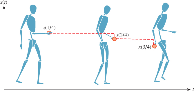
To play the animation we simply alter the mesh vertices according to the input data. Most displays refresh 60–85 times per second (Hz). Because the input is at 4 Hz, if we increment to the next key pose for every frame of animation, then the character will appear to be walking far too fast. For generality, let p = 1/4 s be the period between key poses. Let x(t) = [x(t), y(t), z(t)]T be the position of one vertex at time t. The input specifies this position only at t = k/p for integer values of k; let those values be denoted x*(t). Assume that the same processing will happen to all vertices; we’ll return to ways of accomplishing that in a moment.
If we choose a sample-and-hold strategy for the intermediate frames:
then the animation will play back at the correct rate. The expression for t0 in Equation 35.1 is a common idiom. It rounds t down to the nearest integer multiple of p.
Closely related to sample-and-hold is nearest-neighbor, where we round t to the nearest integer multiple of p.
(a) Write an expression for the nearest-neighbor strategy.
(b) Explain why sample-and-hold, given values at integer multiples of p, is the same as nearest-neighbor applied to the same values, each shifted by p/2. Because of this close relation, the terms are often informally treated as synonyms.
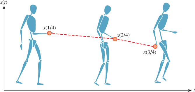
As shown in Figure 35.6, the result of sample-and-hold interpolation will not be smooth. At 60 Hz playback, we’ll see a single pose hold for 15 frames and then the character will instantaneously jump to the next key pose. We can improve this by linearly interpolating between frames:
The linear interpolation avoids the jumps between poses so that positions appear to change smoothly, as shown in Figure 35.7.
This discussion was for a single vertex. There are several methods for extending the derivation to multiple vertices; here are three. A straightforward extension is to apply equivalent processing to each element of an array of vertices. That is, to let xi(t) be the position of the vertex with index i and then let
This array representation for the motion equations matches both the indexed trimesh representation and many real-time rendering APIs, so it is a natural way to approach mesh animation.
One alternative is to leave the interpolation equation (Equation 35.4) unmodified and instead redefine the input and output. For example, we could define a function X(t) describing the state of the system as a very long column comprising the positions of all vertices, instead of a 3-vector-valued function defining a single position:
Note that nothing in our derivation depends on how components are arranged within the vector. Therefore, any two state vectors obeying the same convention can be linearly combined and the components will correspond along the appropriate axes. This representation works well when extending the linear interpolation to splines and, as shown later in this chapter in numerical integration schemes. The chosen interpolation algorithm will simply treat its input and output as a single very high-dimensional point, even though we consider it to be a concatenated series of mesh vertices.
Another alternative is to redefine the position function as a matrix,

This representation works well with the matrix representation of coordinate transformations because we can compute transformations of the form M · X(t), where M is a 4 × 4 matrix.
Each of these representations could be implemented with exactly the same layout in memory. The difference in choice of representation affects the theoretical tools we can bring to bear on animation problems and the practical interface to the software implementation of our algorithms. In practice, representations analogous to each of these have specific applications in animation for different tasks.
In closing, consider the state of our evolving interpolation algorithm. Although the vertex motion is continuous under linear interpolation, there are several remaining problems with this simple key pose interpolation strategy.
• The vertex motion has has C0 continuity. This means that although positions change continuously, the magnitude of acceleration of the vertices is zero at times between poses, and infinite at the time of the key poses. Using a spline with C1 or higher continuity can improve this (see Figure 35.8).
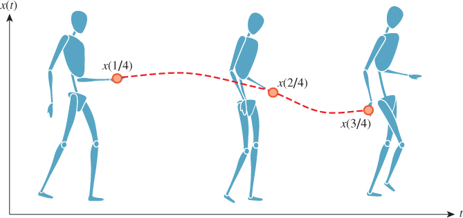
Figure 35.8: Piecewise-cubic interpolation of position over time of a point on a character’s hand using a spline.
• The animation does not preserve volume. Consider key poses of a character and the character rotated 180° about an axis. Linear, or even spline, interpolation will cause the character to flatten to a line and then expand into the new pose, rather than turning.
• The walk cycle doesn’t adapt to the underlying surface on which the character is walking. If the character walks up a hill or stairs, then the feet will either float or penetrate the ground.
• Animations are smooth within themselves, but the transitions between different animations will still be abrupt.
• We can’t control different parts of the character independently. For example, we might want to make the arms swing while the legs walk.
• The animation scheme doesn’t provide for interaction or high-level control. There is no notion of an arm or a leg, just a flat array of vertices.
• We still require a strategy for creating animation data, either by hand or as measurements of real-world examples.
• We’ve only considered animation that is tied to a specific mesh. Creating animation proves to be time-consuming by current practices, so it is desirable to transfer animation of one mesh to a new mesh representing a different character—doing so means abstracting the animation away from the vertices to higher-level primitives like limbs. (The mesh deformation transfer described in Section 25.6.1 is one technique for this.)
Create a simple animation data format and playback program to explore these ideas. Instead of a 3D character, limit yourself to a 2D stick figure. Use only four frames of animation for the walk cycle, and manually enter the key pose vertex positions in a text file. Making even four frames of animation will probably be challenging. Why? What kind of tool could you build to simplify the process? What aspects of the linear interpolation are dissatisfying during playback?
35.2.2. Firing a Cannon (Simulation)
Let’s render an animation of a sailing ship firing a cannon as shown in Figure 35.9. The cannonball will be rendered as a black sphere, so we can ignore its orientation and focus only on the motion of its center of mass/local coordinate frame origin—the root motion. Neglecting the effects of drag due to wind and the slight variance in gravitational acceleration, the cannonball experiences only constant acceleration due to gravity after it is fired. A physics textbook gives an equation for the motion of an object under constant acceleration as
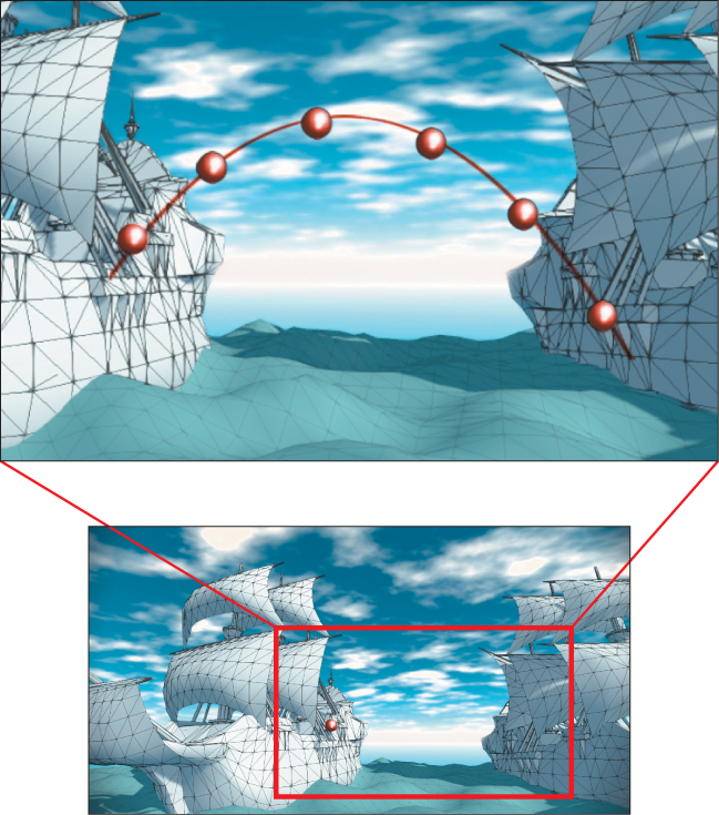
Figure 35.9: One frame (bottom) and a superimposed detail of a sequence of frames (top) of animation depicting the flight of a cannonball as computed by procedural physics.
where x(t) is the 3D position, t is time, x0 = x(0) is the initial position of the object, v0 is the initial velocity of the object, and a0 is the constant acceleration factor. In m-kg-s SI units, position is measured in meters, time in seconds, velocity in meters per second, and acceleration in meters per second squared. The same textbook gives the acceleration from the Earth’s gravitational field as 9.81 m/s2 (downward). We’ll see where these equations and constants came from later in this chapter; for now, let’s just trust the physics textbook. An 18th-century ship’s cannon with an 11 kg ball has a 520 m/s muzzle velocity. Assuming that y is up and we are firing along the x-axis at an elevation of π/4 from the horizontal, the initial conditions are
To actually render an animation, we must produce many individual images separated by small steps in t (see Figure 35.9). When these are quickly viewed consecutively, the viewer will no longer perceive the individual images and instead will see the cannonball moving smoothly through the air. The code to actually render a T-second animation of N individual frames looks something like Listing 35.1.
Listing 35.1: Immediate-mode rendering for a cannonball’s flight.
1 float speed = 520.0f;
2 float angle = 0.7854f;
3
4 Vector3 x0 = ball.position();
5 Vector3 v0(cos(angle) * speed, sin(angle) * speed, 0.0f);
6 Vector3 a0(0, -9.8f, 0);
7
8 for (int i = 0; i < N; ++i) {
9 float t = T * i / (N - 1.0f);
10 ball.setPosition(x0 + v0 * t + 0.5 * a0 * t * t);
11
12 clearScreen();
13 render();
14 swapBuffers();
15 }
The swapBuffers call is important. If we simply cleared the screen and drew the scene repeatedly the viewer would see a flickering as the image was built up with each frame. So we instead maintain two framebuffers: a static front buffer that displays the current frame to the viewer and a back buffer on which we are drawing the next frame. The swapBuffers call tells the rendering API that we are done rendering the next frame so that it can swap the contents of the buffers and show the frame to the viewer. This is called double-buffered rendering.
This was a simple example of procedural motion based on real-world dynamics. The steps here produce a satisfying animation but raise questions that we’ll need to address in a more general framework for procedural motion and dynamics.
• Our equations don’t take into account skipping the cannonball off the surface of the water, sinking it into the water, or crashing it into the targeted ship. How can we detect and respond to collisions and changing circumstances?
• We can solve for the flight time T based on the intersection of the parabolic arc and the other ship (or the water plane). But how should we choose the number of frames N to render in that time?
• What about objects that don’t have constant acceleration from a single force such as gravity? For example, how do we move the ship itself through the water?
• For a featureless ball, we could ignore orientation. What are the equations of motion for an arbitrary tumbling object?
• Imagine procedural motion for an object not moving ballistically (e.g., a person dancing [PG96]). Deriving the equations of motion from first principles of physics would be really hard, and it would also be hard to ask an animator to specify the motion with explicit equations. What can we do?
35.2.3. Navigating Corridors (Motion Planning)
Consider the motion of a hovering robotic drone patrolling the interior of a building (Figure 35.10). We chose a hovering robot to avoid issues of rotating wheels or limbs, and a deforming mesh. The entire motion of the robot can be expressed as a change of the reference frame in which its rigid mesh is defined. This reference frame is called the root frame of the robot and the motion is called root frame animation. (This is a case where context determines the meaning of overloaded technical terminology for motion. The word “frame” in the previous sentence refers to a coordinate transformation, not an image; and “animation” refers to the true 3D motion, not a sequence of images.)
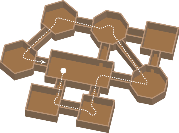
Figure 35.10: Selecting the key poses to navigate a character through these corridors is a problem at the interface between computer graphics and artificial intelligence (based on figure from [AVF04], which discusses AI-based methods for motion planning.).
If we assume that the robot is a uniform sphere in order to ignore the problem of representing its rotational frame, the robot’s animation is simply a formula for the translation of its root frame, x(t) = .... We could approach this problem as either key pose interpolation or a simulation. A hybrid strategy is often best for problems like this: Given an ideal path based on key poses, simulate the actual motion of the robot close to that path based on forces like gravity, the hover mechanism, and drag. This captures both the high-level motion and the character of real physics.
What is the source of the key poses? For a character’s walk cycle, we were able to assume that an animator used some tool to create the key poses. To accurately model an autonomous robot, or to create an interactive application, we can’t rely on an artist. The robot must choose its own key poses dynamically based on a goal, such as navigating to a specific room. This is an Artificial Intelligence (AI) problem. Real-world robots and video games with nonplayer characters solve it, generally using some form of path finding algorithm. Path finding has been long studied in computer science, primarily in the context of abstract graphs. For a 3D virtual world we must solve not only the graph problem but also the local problems that arise from actual room geometry and multiple interacting characters. A common approach is to apply a traditional AI path finding algorithm like A * to create a root motion spline, and then use another greedy algorithm to look ahead a small time interval and avoid small-scale collisions.
So far, we have considered only translational root motion for navigation. The problem of synthesizing dynamic character motion becomes even more challenging when we must solve for the motion of limbs, coordinate multiple characters, or handle deformation. This general problem is called motion planning, and it is an active area of research in not only computer graphics but also AI and robotics. Most solutions draw on the principles and algorithms described in this chapter. However, they also tend to leverage search and machine learning strategies that require more AI background to describe. Having motivated it, we now leave the motion planning aside. The remainder of this chapter overviews basic primitives up to motion in the absence of AI, with emphasis on the motion of rigid primitives.
35.2.4. Notation
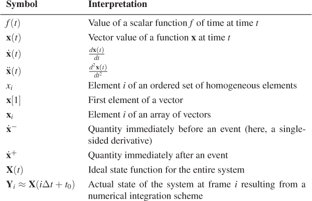
Variables in animation algorithms are qualified in many ways. Reference frames have three translational dimensions and three rotational dimensions, all quantities are functions of time, and most quantities are actually arrays to accommodate multiple objects or vertices. The algorithms we use also typically involve first and second time derivatives, and often consider the instantaneous value before and after an event such as a collision.
Animation-specific notations address these qualifications, but they differ from the notations predominant in rendering that are used elsewhere in this book. The following notation, which is common in the animation literature, applies only within this chapter (see Table 35.1).
Vectors are in boldface (e.g., x), to leave space for other hat decorations. A dot over the x denotes that ![]() is the first derivative of x with respect to time. This is a common notation in physics. In animation, time appears in all equations and is always denoted by t (except when we need temporary variables for integration), so all derivatives are with respect to t (e.g.,
is the first derivative of x with respect to time. This is a common notation in physics. In animation, time appears in all equations and is always denoted by t (except when we need temporary variables for integration), so all derivatives are with respect to t (e.g., ![]() ). Multiple dots indicate higher-order derivatives (e.g.,
). Multiple dots indicate higher-order derivatives (e.g., ![]() ).
).
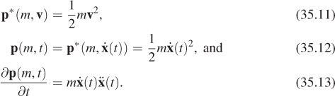
There are two hazards in this dot notation. The first is that “![]() ” is such a compact form that it is easy to drop the “(t)” and treat the value of a velocity expression as a variable instead of as the evaluation of a function. When taking derivatives of complex expressions such as momentum that are based on velocity, forgetting that velocity is a function of time can lead to errors if you forget to apply the chain rule. For example, let’s look at a function of two arguments defined by
” is such a compact form that it is easy to drop the “(t)” and treat the value of a velocity expression as a variable instead of as the evaluation of a function. When taking derivatives of complex expressions such as momentum that are based on velocity, forgetting that velocity is a function of time can lead to errors if you forget to apply the chain rule. For example, let’s look at a function of two arguments defined by ![]() (which happens to be the momentum equation). We can compute the partial derivatives,
(which happens to be the momentum equation). We can compute the partial derivatives, ![]() ;
; ![]() . What you might see in an animation paper is a description of this function where the author writes, “
. What you might see in an animation paper is a description of this function where the author writes, “![]() .” And you’ll even see things like “
.” And you’ll even see things like “![]() .” Here,
.” Here, ![]() is being treated as a variable, just like v, and it is almost reasonable to do so thus far. It is also common to see “
is being treated as a variable, just like v, and it is almost reasonable to do so thus far. It is also common to see “![]() .” This is a little strange because t isn’t even one of the arguments of function p, and
.” This is a little strange because t isn’t even one of the arguments of function p, and ![]() has changed from its role as a variable whose symbol happens to have a dot hat to representing a function of time whose time derivative is denoted
has changed from its role as a variable whose symbol happens to have a dot hat to representing a function of time whose time derivative is denoted ![]() . Thus, for clarity, in this chapter when we want such a function, we write either
. Thus, for clarity, in this chapter when we want such a function, we write either ![]() , or more verbosely,
, or more verbosely,
The second notational hazard is that the implementation of a dynamics system often uses higher-order functions. That is, it contains functions that take other functions as their arguments. In programming, the argument functions are called first-class functions or function pointers. There is a real distinction between the vector-valued function x (i.e., Vector3 position(float time) ...) and the vector value of that function at time t, x(t) (i.e., Vector3 currentPosition;). Passing the wrong one as an argument will lead to programming errors. We therefore always keep the derivatives in function notation for this chapter. However, be warned that in the animation literature it is commonplace to move between the variable and function notation.
Here’s one critical example of this notation. When discussing numerical integration schemes that dominate the dynamics portion of this chapter, we distinguish three fundamental representations. The position of an object (which may represent only position, or may be extended with other information) is x(t), which is a vector-valued function. The elements of the vector may be, for example, x-, y-, and z-coordinates, or those coordinates and rotational (and other pose) information. Since there may be many objects in a system, or many points on a single object, we consider a set of functions. When evaluated at t, their values are denoted x1(t), X2(t), etc. The state function of the entire system, which comprises the entire set of position functions and their derivatives, is written X(t) when evaluated at time t. The state function is defined for continuous t.
When we approximate the state function with a numerical integrator that takes discrete steps, we refer to the values of the state function at given step indices. This is Yi ≈ X(iΔt + t0). Note that Yi for a given i is not a function—it is a value, which is typically represented as an array of (3D) vectors in a program. One could alternatively think of a function on a discrete time domain whose value at step i is Y[i]. However, we do not use that notation for two reasons. First, we reserve the bracket notation for referencing the elements of a vector value. Second, a typical implementation only contains one Y value at a time. It would be misleading to think of it as a discrete function or array of values because only a single one is present in memory at a time. A good mental model for Yi is the ith element of a sequence that the program is iterating through, which is what that notation is intended to suggest.
35.2.4.1. Notation in the Big Picture
For what it is worth, the first, and perhaps one of the most significant, challenges in learning the mathematics of animation is simply grappling with the notation. We’ve tried to choose a relatively simple and consistent notation for this chapter, but we acknowledge that it is still a ridiculously large new language to learn for something as seemingly simple as expressing Newton’s laws.
The notation is complex because it bears the burden of expressing the many shades of “position” and values derived from it in a formal computational system. The gist of those shades and derivations embodies the fundamental rules, and thus the power, of animation. The gist is what is important because in a virtual world, the specifics of the laws of physics are arbitrary and mutable. On the computational side, there are a large number of ways to integrate and interpolate values. There is no single best solution (although there are some solutions that are always inferior).
As a concrete example, understanding the inputs and outputs of an integrator is actually more important than understanding the integration algorithm itself. There are many integration algorithms, but they all fit into the same integration systems that dictate the data flow. So the notation really is telling you something important. It therefore is worth taking the time to ensure that you understand the distinction between each x and x in an equation.
35.3. Considerations for Rendering
We now consider several ways in which animation and rendering are interrelated, ranging from display techniques like double and triple buffering to make animation appear smoother, all the way to approaches for generating motion blur to help smooth the appearance of moving objects.
35.3.1. Double Buffering
When a display can refresh faster than the processor can render a frame, drawing directly to the display buffer would reveal the incomplete scene. Because this is generally undesirable, double-buffered rendering draws to an off-screen back buffer while the front buffer containing the previous frame is displayed to the viewer. When the back buffer is complete, the buffers are “swapped,” either by copying the contents of the back to the front or by moving the display’s pointer between the buffers. The cannonball code in Listing 35.1 showed an example of how an explicit call to swap buffers can manage double-buffered rendering. Double-buffered rendering of course doubles the size of the frame-buffer in memory.
Analog vector scope (oscilloscope) displays have no buffer—a beam driven by analog deflection traces true lines on the display surface. So double-buffered rendering is impossible for such displays and they inherently reveal the scene as it is rendered. Vector scopes are rarely used today, although some special-purpose laser-projector displays operate on the same principle and have the same drawbacks.
For displays driven by a digital framebuffer, the swap operation must be handled carefully. A CRT traces through the rasters with a single beam. Pixels in the framebuffer that are written to will not be updated until the beam sweeps back across the corresponding display pixel. LCD, plasma, and other modern flat-screen technologies are capable of updating all pixels simultaneously, although to save cost, a specific display may not contain independent control signals for each pixel. Regardless, the display is typically fed by a serial signal obtained by scanning across the framebuffer in much the same way as a CRT. The result is that for most modern displays the buffers must be swapped between scanning passes. Otherwise, the top and bottom of the screen will show different frames, leading to an artifact called screen tearing. The raster at which the screen is divided will scroll upward or downward depending on the ratio of refresh rate to animation rate.
The solution to tearing is vertical synchronization, which simply means waiting for the refresh to swap buffers. The drawback of this is that it may stall the rendering processor for up to the display refresh period. Two common solutions are disabling vertical synchronization (which entails simply accepting the resultant tearing artifacts) and triple buffering. Under triple buffering, three frame-buffers are maintained as a circular queue. This allows the renderer to advance to the next frame at a time independent of the display refresh. Of course, the renderer must still be updating at about the same rate as the display or the queue will fill or become empty, stalling either the display or the renderer. The queue may be implemented in a straightforward manner as an array of framebuffers that are each used in sequence, or as two double-buffer pairs that share a front buffer. The drawbacks of triple-buffered rendering are further increased framebuffer storage cost and an additional frame of latency between user input and display.
35.3.2. Motion Perception
Motion perception is an amazing property of the human visual system that enables all computer graphics animation. Current biological models of the visual system indicate that there is no equivalent of a refresh rate or uniform shutter in the eye or brain. Yet we perceive the objects in sequential frames shown at appropriate rates as moving smoothly, rather than warping between discrete locations or as separate objects that appear and disappear.
Motion phenomena are believed to occur mostly within the brain. However, the retina does exhibit a tendency to maintain positive afterimages for a few milliseconds and this may interact with the brain’s processing of motion. These are distinct from the negative afterimages that occur when staring at a strong stimulus for a long period of time.
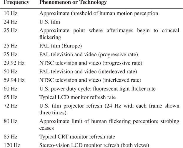
One effect of positive afterimages is that the human visual system is only strongly sensitive to flickering due to shuttering or image changes up to about 25 Hz, and is completely insensitive to flickering at frequencies higher than 80 Hz. This is partly why the 50 Hz (Europe) or 60 Hz (U.S.) flickering of a fluorescent light is just barely perceptible, and is why most computer displays refresh at 60 to 85 Hz.
The Beta phenomenon [Wer61], sometimes casually referred to by the overloaded term “persistence of vision,” is the phenomenon that allows the brain to perceive object movement. At around 10 Hz, the threshold of motion perception is crossed and overlapping objects in sequential frames may appear to be a single object that is in motion. This is only the minimum rate for motion perception. If the 2D shapes are not suitably overlapped they will still appear as separate objects. This means that fast-moving objects in screen space require higher frame rates for adequate presentation.
The combination of fast-moving objects and the limitations of afterimages to conceal flickering cause a phenomenon called strobing. Here, motion perception breaks down even at frame rates higher than 30 Hz. A classic example of strobing is a filmed or rendered roller-coaster ride from a first-person perspective. Because points on the coaster track can traverse a significant portion of the screen, even at high frame rates the individual frames may appear as actual separate flashing images and not blend into perceived motion of an object. This can be a disturbing artifact that causes nausea or headache if prolonged. Above 80 Hz, afterimages appear to completely conceal the strobing effect and the motion becomes apparent, although the actual images may be blurred by the visual system.
The human perception of motion and flickering creates a natural range for viable animation rates, from about 10 Hz to about 80 Hz. Table 35.2 shows that various solutions are currently in use throughout that viable range.
We note that for dynamics, the rendering rate may be independent of the simulation rate. Simulating at low rates and then interpolating between simulation steps when rendering amortizes the cost of a simulation step. Simulating at high rates and then subsampling simulation steps when rendering can increase accuracy and stability. We return to these issues later in this chapter.
Most LCD monitors refresh at around 60–65 Hz, although some displays refresh at 120 or 240 Hz for shuttered stereo viewing of 60 Hz or 120 Hz images.
Note that there are two standards for film: 24 Hz in the United States and Japan and 25 Hz for the PAL/SECAM standard used in Europe and the rest of Asia. Interestingly, projected films are typically not adapted to the display’s frame rate when moving between PAL and NTSC standards. Thus, 25 Hz European films are screened in the United States at 24 Hz. The audio makes the corresponding 4% speed change to remain in synchrony. The net result is that European films appear slow and low-pitched while American films appear fast and high-pitched, when viewed in the opposite projection mode.
35.3.3. Interlacing
Many television broadcast and storage formats are interlaced. In an interlaced format, each frame contains the full horizontal resolution of the final image but only half the vertical resolution. These half-resolution frames are called fields. Even and odd fields are offset by one pixel (or historically, one scan line). To display a complete image, two sequential fields must be combined by interlacing their rasters (rows of pixels).
Because each image merges pixels from different time slices, no single image is consistent. However, fast motion can be represented at comparatively low bandwidth. The artifacts of interlacing were historically hidden by the decay time of CRT phosphors, which took longer to change intensity than the frame period. Some contemporary displays can change images rapidly and thus reveal the interlacing pattern. This can be observed when pausing playback on an LCD monitor, although some displays attempt to interpolate between adjacent frames to reconstruct a progressive signal from an interlaced one.
At the time of this writing, most broadcast television and archived television shows remain in interlaced formats. With the advent of high-definition digital displays, new content is increasingly moving to progressive formats. Progressive is what you would expect: Each frame contains a complete image.
The progressive rate for PAL/SECAM television is 25 Hz and the interlaced rate is 50 Hz. This means that normal European television broadcasts send one field every 1/50 s such that every 1/25 s a complete image has been transmitted.
Console games displayed on televisions may elect to render in either progressive or interlaced formats. The advantage of an interlaced format is that there are half as many pixels to render per frame, yet the viewer rarely perceives a 50% reduction in quality.
35.3.3.1. Telecine
The PAL/SECAM formats allow European films to be broadcast unmodified on European television because they both are driven at 25 Hz. To interlace such a film, simply drop half the rasters each frame.
In the United States, the process is not as simple. NTSC television requires approximately 30 Hz, but U.S. films are at 24 Hz. These only align once every six frames, and interpolating the remaining frames from adjacent ones would significantly blur the images. The telecine or pulldown employed in practice is a clever alternative that exploits interlacing.
The commonly employed algorithm is called 3:2 pulldown. We begin with a simplified example to understand the intuition behind it. Instead of resampling from 24 Hz progressive to 30 Hz progressive, consider the problem of resampling from 24 Hz progressive to 60 Hz interlaced. We can approach this by replicating each source frame “2.5” times, that is, by repeating frame i twice, blending frames i and i + 1, and then proceeding to process frame i + 1. This blends only one out of every three frames, which is substantially better than blending five out of every six frames. The output will be progressive, so to create an interlaced format, drop half the rasters from every frame.
What the actual 3:2 pulldown algorithm does is perform the blending by choosing the source rasters more selectively. This avoids blending pixels from separate frames and directly produces interlaced output. This is similar to stochastic blending methods like dithering: The blending is spatial and is integrated by the eye. Figure 35.11 shows the process. Given four original film frames A, B, C, and D sampled at 24 Hz (left column), the algorithm will produce 4 · 2.5 = 10 interlaced frames at ≈60 Hz (center columns), that correspond to five progressive frames at ≈30 Hz (right column). Note that the interlaced frames are broadcast in alternating raster order, so the top frame of the left-center column will be broadcast first, followed by the top frame of the right-center column, followed by the second-to-top row of the left-center column, etc.
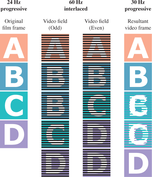
Figure 35.11: Schematic of how interlacing is exploited to adapt 24 Hz film frames for 60 Hz interlaced broadcast to NTSC televisions under the 3:2 pulldown algorithm. In the center columns, the odd and even source film frames have been repeated three and two times, respectively. (Created by Eric Lee.)
The interlaced frames are chosen by repeating even frames from the original film twice and odd frames from the film three times; that is, odd to even appear in the ratio 3:2. Notice how in the center columns the even source frames A and C appear twice and the odd source frames B and D appear three times.
35.3.4. Temporal Aliasing and Motion Blur
Rendering a frame from a single instant in time is convenient because all geometry can be considered static for the duration of the frame. Each pixel value in an image represents an integral over a small amount of the image plane in space and a small amount of time called the shutter time or exposure time. Film cameras contained a physical shutter that flipped or irised open for the exposure time. Digital cameras typically have an electronic shutter. For a static scene, the measured energy will be proportional to the exposure time. A virtual camera with zero exposure can be thought of as computing the limit of the image as the exposure time approaches zero.
There are reasons to favor both long and short exposure times in real cameras. In a real camera, short exposure times lead to noise. For moderately short exposure times (say, 1/100 s) under indoor lighting, background noise on the sensor may become significant compared to the measured signal. For extremely short exposure times (say, 1/10,000 s), there also may not be enough photons incident on each pixel to smooth out the result. Nature itself uses discrete sampling because photons are quantized. In computer graphics we typically consider the “steady state” of a system under large numbers of photons, but this model breaks down for very short measurement intervals. A long exposure avoids these noise problems but leads to blur. For a dynamic scene or camera, the incident radiance function is not constant on the image plane during the exposure time. The resultant image integrates the varying radiance values, which manifest as objects blurring proportional to their image space velocity. Small camera rotations due to a shaky hand-held camera result in an entirely blurry image, which is undesirable. Likewise, if the screen space velocity of the subject is nonzero, the subject will appear blurry. This motion blur can be a desirable effect, however. It conveys speed. A very short exposure of a moving car is identical to that of a still car, so the observer cannot judge the car’s velocity. For a long exposure, the blur of the car indicates its velocity. If the car is the subject of the image, the photographer might choose to rotate the camera to limit the car to zero screen-space velocity. This blurs the background but keeps the car sharp, thus maintaining both a sharp subject and the velocity cue.
For rendering, our photons are virtual and there is no background noise, so a short exposure does not produce the same problems as with a real camera. However, just as taking only one spatial sample per pixel results in aliasing, so does taking only one temporal sample. The top row of Figure 35.12 shows two images of a very thin row of bars, as on a cage. If we take only one spatial sample per pixel, say, at the pixel center, then for some subpixel camera offsets the bars are visible and for others they are invisible. Note that as the spatial sampling density increases, the bars can be resolved at any position. The bottom row shows the result of the equivalent experiment performed for temporal samples. A fast-moving car is driving past the camera in the scene depicted. For a single temporal sample, the car may be either present or absent. Increasing the temporal sampling rate increases the ability to resolve the car. For a high temporal sampling rate the image approaches that which would be captured by a real camera, where the car is blurred across the entire frame.
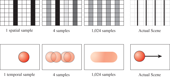
Figure 35.12: Top row: a fence made of black posts on a white background imaged with increasing spatial resolution. Bottom row: a moving sphere imaged with increasing temporal resolution. Increasing the number of samples better captures the underlying scene, in space or time. Here a regular sampling pattern is used for each.
One method for ameliorating temporal aliasing is to use a high-refresh rate display and render once per refresh. Although not common today, there are production 240 Hz displays. Simply rendering at 240 Hz provides four times the temporal sampling rate of the common 60 Hz rendering rate. This does not solve the temporal aliasing problem. It merely reduces its impact. A sufficiently fast car, for example, will still flash into the center of the screen and disappear.
A more common alternative to a high refresh rate solves the flashing problem and does not require a special display. One can explicitly integrate many temporal samples, producing rendered motion blur. Distribution1 ray tracing [CPC84] pioneered this approach, which has since been extended to rasterization. Here, software is performing the integration that was performed by the eye under a high-refresh display.
1. Cook et al. originally called their technique “distributed” ray tracing because it distributes samples across the sampling domain, including time. Today it is commonly called “distribution” ray tracing to distinguish it from processing distributed across multiple computers. It is also called “stochastic” ray tracing since it is often implemented using stochastic sampling, although technically, the decision to distribute samples (especially eye-ray samples) is separate from the choice of sampling pattern.
Integration over temporal samples does not necessarily give the same perception as observing a high refresh display or the real world, however. The reason is that the eye is not a camera. In the absence of temporal integration, the observer’s eye can track the motion of an object in the scene at a high rate. For example, the eye can rotate to keep an object moving across the display’s field of view at the same location in the eye’s field of view. The resultant perception is that the moving object is sharp and the background is blurred. If the same scene is shown at a low frame rate that has been integrated over multiple temporal samples, the moving object will be blurred and the background will be sharp. This might lead one to the conclusion that motion blur cannot be rendered effectively without eye tracking. However, all live-action film faces exactly this problem and rarely do viewers experience disorientation at the fact that the images have been preintegrated over time for their eyes. If the director does a good job of directing the viewer’s attention, the camera will be tracking the object of primary interest in the same way that the eye would. Presumably, a poorly directed film fails at this and creates some disorientation, although we are not aware of a specific scientific study of this effect. Similar problems arise with defocus due to limited depth of field and with stereoscopic 3D. For interactive 3D rendering all three effects present a larger challenge because it is hard to control or predict attention in an interactive world. Yet in recent years, games in particular have begun to experiment with these effects and achieve some success even in the absence of eye tracking.
Antialiasing, motion blur, and defocus are all cases of integrating over a larger sampling area than a single point to produce synthetic images that more closely resemble those captured by a real camera. Many rendering algorithms combine these into a “5D” renderer, where the five dimensions of integration are subpixel x, y, time, and lens u, v. Cook et al.’s original distribution and stochastic ray tracing schemes [CPC84, Coo86] can be extended to statistically dependent temporal samples per pixel by simply rendering multiple frames and then averaging the results. Because all samples in each frame are at the same time, for large motions this produces discrete “ghosts” for fast-moving objects instead of noisy ghosts, as shown in Figure 35.13. Neither of these is ideal—the image has been undersampled in time and each is a form of aliasing. The advantage of averaging multiple single-time frames is that any renderer, including a rasterization renderer, can be trivially extended to simulate motion blur in this method.
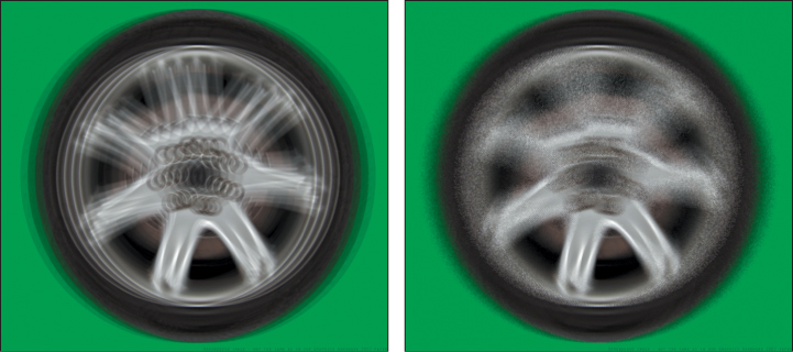
Figure 35.13: Undersampling in time with regular (a.k.a. uniform, statistically dependent) samples within each pixel (left) produces ghosting. Undersampling with stochastic (a.k.a. independent, random) samples produces noise (right) [AMMH07]. (Courtesy of Jacob Munkberg and Tomas Akenine-Möller)
The Reyes micropolygon rendering algorithm [CCC87] that has been heavily used for film rendering is a kind of stochastic rasterizer. It takes multiple temporal samples during rasterization to produce effects like motion blur, avoiding the problem of dependent time samples. Akenine-Möller et al. [AMMH07] introduced explicit temporal stochastic rasterization for triangles, and Fatahalian et al. [FLB+09] combined that idea with micropolygons for full 5D micropolygon rasterization. Fatahalian et al. framed rasterization as a five-dimensional point-inpolyhedron problem and solved it in a data-parallel fashion for efficient execution on dedicated graphics hardware.
Because integration over multiple samples is expensive, a variety of tricks that generate phenomena similar to motion blur have been proposed. These have historically been favored by the game industry because they are fast, if sometimes poor-quality, approximations. See Sung et al. [SPW02] for a good survey of these. The major methods employed are adding translucent geometry that stretches an object along its screen-space velocity vector, artificially increasing the MIP level chosen from textures to blur within an object, and screen-space blurring based on per-pixel velocity as a post-process [Vla08].
Renderers paradoxically spend more time producing blurry phenomena such as motion blur than they do in imaging sharp objects. This is because blurring requires either multiple samples or additional post-processing. Since it is harder for viewers to notice artifacts in blurry areas of an image, it would be ideal to somehow extrapolate the blurry result from fewer samples. This is currently an active area of research [RS09, SSD+09, ETH+09].
35.3.5. Exploiting Temporal Coherence
An animation contains multiple frames, so rendering animation is necessarily more computationally intense than rendering a single image. However, the cost of rendering an animation is not necessarily proportional to its length. Sequential frames often depict similar geometry and lighting viewed through similar cameras. This property is referred to as frame coherence or temporal coherence. It may hold for the underlying scene state, the rendered image, both, or neither.
One advantage of frame coherence is that one can often reuse intermediate results from rendering one frame for the subsequent frame. Thus, the first frame of animation is likely as expensive to render as a single image, but subsequent frames may be comparatively inexpensive to render.
For example, it is common practice in modern rasterization renderers to only recompute the shadow map associated with a luminaire only when both the volume illuminated by that luminaire intersects the view frustum and something within that volume moved since the previous computation. Historically, 2D renderers were not fast enough to update the entire screen when drawing user interfaces. They exploited frame coherence to provide a responsive interface. Such systems maintained a persistent image of the screen and a list of 2D bounding boxes for areas that required updating within that image. These bounding boxes were called dirty rectangles. Although modern graphics processors are fast enough to render the entire screen every frame, the notion of dirty rectangles and its generalization to dirty bit flags remains a core one for incremental updates to computer graphics data structures.
The process of storing intermediate results for later reuse is generally called memoization; it is also a main component of the dynamic programming technique. If we allow only a fixed-size buffer for storing previous results and have a replacement strategy when that buffer is full, the process is called caching. Reuse necessarily requires some small overhead to see if the desired result has already been computed. When the desired result is not available (or is out of date, as in the dirty rectangle case) the algorithm has already invested the time for checking the data structure and must now pay the additional time cost of computing the desired result and storing it. Storing results of course increases the space cost of an algorithm. Thus, reuse strategies can actually increase the total cost of rendering when an animation fails to exhibit frame coherence.
When reuse produces a net time savings, it is reducing the amortized cost of rendering each frame. The worst-case time may still be very high. This is problematic in interactive applications, where inconsistent frame intervals can break the sense of immersion and generally hampers continuous interaction. One solution is to simply terminate rendering a frame early when this occurs. For example, the set of materials (i.e., textures) used in a scene typically changes very little between frames, so the cost of loading them is amortized over many frames. Occasionally, the material set radically changes. This happens, for example, when the camera crests a hill and a valley is revealed. One can design a renderer that simply renders parts of the scene for which materials are not yet available with some default or low-resolution material. This will later cause a visual pop (violating coherence of the final image) when these materials are replaced with the correct ones, but it maintains the frame rate. The worst case is often the first frame of animation, for which there is no previous frame with which to exhibit coherence.
35.3.6. The Problem of the First Frame
The first frame of animation is typically the most expensive. It may cost orders of magnitude more time to render than subsequent frames because the system needs to load all of the geometry and material data, which may be on disk or across a network connection. Shaders have not yet been dynamically compiled by the GPU driver, and all of the hardware caches are empty. Most significantly, the initial “steady state” lighting and physics solution for a scene is often very expensive to compute compared to later incremental updates.
Today’s video games render most frames at 1/30 s or 1/60 s intervals. Yet the first frame might take about one minute to render. This time is often concealed by loading data on a separate thread in the background while displaying a loading screen, prerendered cinematic, or menus. Some applications continuously stream data from disk.
If we consider the cost of precomputed lighting, some games take hours to render the first frame. This is because computing the global illumination solution is very expensive. The result is stored on disk and global illumination is then approximated for subsequent frames by the simple strategy of assuming it did not change significantly. Although games increasingly use some form of dynamic global illumination approximation, this kind of precomputation for priming the memoization structure is a common technique throughout computer graphics.
Offline rendering for film is typically limited by exactly these “first frame” problems. Render farms for films typically assign individual frames to different computers, which breaks coherence on each computer. Unlike interactive applications, at render time films have prescripted motion, so the “working set” for a frame contains only elements that directly affect that frame. This means that even within a single shot, the working set may exhibit much less coherence than for an interactive application. Because of this system architecture and pipeline, a film renderer is in effect always rendering the first frame, and most film rendering is limited by the cost of fetching assets across a network and computing intermediate results that likely vary little from those computed on adjacent nodes.
35.3.7. The Burden of Temporal Coherence
When rendering an animation where the frames should exhibit temporal coherence, an algorithm has the burden of maintaining that coherence. This burden is unique to animation and arises from human perception.
The human visual system is very sensitive to change. This applies not only to spatial changes such as edges, but also to temporal changes as flicker or motion. Artifacts that contribute little perceptual error to a single image can create large perceptual error in an animation if they create a perception of false motion. Four examples are “popping” at level-of-detail changes for geometry and texture, “swimming jaggies” at polygon edges, dynamic or screen-door high-frequency noise, and distracting motion of brushstrokes in nonphotorealistic rendering,
Popping occurs when a surface transitions between detail levels. Because immediately before and immediately after a level-of-detail change either level would produce a reasonable image, the still frames can look good individually but may break temporal coherence when viewed sequentially. For geometry, blending between the detail levels by screen-space compositing, subdivision surface methods (see Chapter 23), or vertex animation can help to conceal the transition. Blending the final image ensures that the final result is actually coherent, whereas even smoothly blending geometry can cause lighting and shadows to still change too rapidly. However, blending geometry guarantees the existence of a true surface at every frame. Image compositing results in an ambiguous depth buffer or surface for global illumination purposes. For materials, trilinear interpolation (see Chapter 20) is the standard approach. This generates continuous transitions and allows tuning for either aliasing (blurring) or noise. A drawback of trilinear interpolation is that it is not appropriate for many expressions, for example, unit surface normals.
Sampling a single ray per pixel produces staircase “jaggies” along the edges of polygons. These are unattractive in a still image, but they are worse in animation where they lead to a false perception of motion along the edge. The solution here is simple: antialiasing, either by taking multiple samples per pixel or through an analytic measure of pixel coverage.
High-frequency, low-intensity noise is rarely objectionable in still images. This property underlies the success of half-toning and dithering approaches to increasing the precision of a fixed color gamut. However, if a static scene is rendered with noise patterns that change in each frame, the noise appears as static swimming over the surfaces in the scene and is highly objectionable.
The problem of dynamic noise patterns arises from any stochastic sampling algorithm. In addition to dithering, other common algorithms that are susceptible to problems here include jittered primary rays in a ray tracer and photons in a photon mapper. Three ways to avoid this kind of artifact are making the sampling pattern static, using a hash function, and slowly adjusting the previous frame’s samples.
Supersampling techniques for antialiasing often rely on the static pattern approach. This can be accomplished by stamping a specific pattern in screen space. There has been significant research into which patterns to use [GS89, Coo86, Cro77, Mit87, Mit96, KCODL06, Bri07, dGBOD12]. This work is closely tied to research on white noise random number generation [dGBOD12].
One drawback to using screen-space patterns is the screen door effect (Chapter 34). A static pseudorandom pattern in screen space is not perceptible in a single image, but when the pattern is held fixed in screen space and the view or scene is dynamic, that pattern becomes perceptible. It looks as if the scene were being viewed through a screen door. This is easy to see in the real world. Hold your head still and look through a window (or slightly dirty eyeglasses). The glass is largely invisible, but on moving your head imperfections in and dirt on the glass are accentuated. This is because your visual system is trying to enforce temporal coherence on the objects seen through the glass. Their appearance is changing in time because of the imperfections in the glass in front of them, so you are able to perceive those imperfections.
Fortunately, when the sampling pattern resolution falls below the resolution of visual acuity, the perception of the screen-door effect is minimal. This is exploited by supersampling and alpha-to-coverage transparency, which operate below the pixel scale and are therefore inherently close to the smallest discernible feature size. Dithering works well when the image is static or the pixels are so small as to be invisible, but it produces a screen-door effect for animations rendered to a display with large pixels.
It is challenging to stamp patterns in continuous spaces; for example, a ray tracer or photon mapper’s global illumination scattering samples. Here, replacing pseudorandom sampling with sampling based on a hash of the sample location is more appropriate. By their very nature, hash functions tend to map nearby inputs to disparate outputs, so this only maintains coherence for static scenes with dynamic cameras. For dynamic scenes, a spatial noise function is preferable [Per85] because it is itself spatially coherent, yet pseudorandom.
Another approach to increasing temporal coherence of sample points is to begin with an arbitrary sample set and then move the samples forward in time, adding and removing samples as necessary. This approach is employed frequently for nonphotorealistic rendering. The Dynamic Canvas [CTP+03] algorithm (Figure 35.14) renders the background paper texture for 3D animations rendered in the style of natural media. A still frame under this algorithm appears to be, for example, a hand-drawn 3D sketch on drawing paper. As the viewer moves forward, the paper texture scales away from the center to avoid the screen-door effect and give a sense of 3D motion. As the viewer rotates, the paper texture translates. The algorithm overlays multiple frequencies of the same texture to allow for infinite zoom and solves an optimization problem for the best 2D transformation to mimic arbitrary 3D motion. The initial 2D transformation is arbitrary, and at any point in the animation the transformation is determined by the history of the viewer’s motion, not the absolute position of the viewer in the scene.
Figure 35.14: The Dynamic Canvas algorithm [CTP+03] produces background-paper detail at multiple scales that transform evocatively under 3D camera motion. (Courtesy of Joelle Thollot, “Dynamic Canvas for Non-Photorealistic Walk-throughs,” by Matthieu Cunzi, Joelle Thollot, Sylvain Paris, Gilles Debunne, Jean-Dominique Gascuel and Fredo Durand, Proceedings of Graphics Interface 2003.)
Another example of moving samples is brushstroke coherence, of the style originally introduced for graftals [MMK+00] (see Figure 35.15). Graftals are scene-graph elements corresponding to strokes or collections of strokes for small-detail objects, such as tree leaves or brick outlines. A scene is initially rendered with some random sampling of graftals; for example, leaves at the silhouettes of trees. Subsequent frames reuse the same graftal set. When a graftal has moved too far from the desired distribution due to viewer or object motion, it is replaced with a newly sampled graftal. For example, as the viewer orbits a tree, graftals moving toward the center of the tree in the image are replaced with new graftals at the silhouette. Of course, this only amortizes the incoherence, because there is still a pop when the graftal is replaced. Previously discussed strategies such as 2D composition can then reduce the incoherence of the pop.

Figure 35.15: The view-dependent tufts on the trees, grass, and bushes are rendered with graftals that move coherently between adjacent frames of camera animation. (Courtesy of the Brown Graphics Group, ©2000 ACM, Inc. Reprinted by permission.)
An open question in expressive rendering is the significance of temporal coherence for large objects like strokes. On the one hand, we know that their motion is visually distracting. On the other hand, films have been made with hand-drawn cartoons and live-action stop motion in the past. There, the incoherence can be considered part of the style and not an artifact. Classic stop-motion animation involves taking still images of models that are then manually posed for the next frame. When the stills are shown in sequence, the models appear to move of their own volition because the intermediate time in which the animator appeared in the scene to manipulate it is not captured on film.
35.4. Representations
We now talk about animation methods, the naming of parts of animatable models, and alternatives among which one might choose to express the parameters and computational model of animation.
The state of an animated object or scene is all of the information needed to uniquely specify its pose. For animation, a scene representation must encompass both the state and a parameterization scheme for controlling it. For example, how do we encode the shape and location of an apple and the force of gravity on it?
As is the case in rendering, one generally wants the simplest representation that can support plausible simulation of an object. For rendering, interaction with light is significant, so the surface geometry and its reflectance properties must be fairly detailed. For animation, interaction with other objects is significant, so properties like mass and elasticity are important. Animation geometry may be coarse, and different from that used for rendering. A variety of animation representations have been designed for different applications. This chapter references many and explores particles and fluid boundaries in depth as case studies.
We categorize schemes for parameterizing, and thus controlling, state into key poses created by an artist, dynamics simulation by the laws of physics, and explicit procedures created by an artist-programmer. Many systems are hybrids. These leverage different control schemes for different aspects of the scene to accommodate varying simulation level of detail or artistic control.
35.4.1. Objects
The notion of an object is a defining one for an animation system. For example, by calling an automobile an “object” one assumes a complex simulation model that abstracts individual systems. If one instead considers an individual gear as an “object,” then the simulation system for an automobile is simple but has many parts. This can be pushed to extremes: Why not consider finite elements of the gears themselves, or molecules, or progress the other way and consider all traffic on a highway to be one “object”?
The choice of object definition controls not only the complexity of the underlying simulation rules, but also what behaviors will emerge naturally versus requiring explicit implementation. For example, finite-element objects might naturally simulate breaking and deformation of gears and bricks, whereas atomic gear or brick objects cannot break without explicit simulation rules for creating new objects from their pieces.
How much complexity do we need to abstract the behaviors of scenes that we might want to simulate? A tumbling crate retains a rigid shape relative to its own reference frame, but that frame moves through space. A walking person exhibits underlying articulated skeleton of rigid bones connected at joints that are then covered by deforming muscle and skin. The water in a stream lacks any rigid substructure. It deforms around obstacles and conforms to the shape of the stream bed under forces including gravity, pressure, and drag.
In each of these scenarios, the objects involved have varying amounts of state needed to describe their poses and motion. The algorithms for computing changes of that state vary accordingly.
Some object representations commonly employed in computer graphics (with examples) are
1. Particles (smoke, bullets, people in a crowd)
2. Rigid body (metal crate, space ship)
3. Soft rigid body (beach ball)
4. Articulated rigid body (robot)
5. Mass-spring system (cloth, rope)
6. Skinned skeleton (human)
7. Fluid (mud, water, air)
These are listed in approximate order of complexity and algorithmic state. For example, the dynamic state of a particle consists of its position and velocity. A rigid body adds a 3D orientation to the particle representation.
Why are so many different representations employed? As an alternative, a single unified representation would be much more theoretically appealing, be easier from a software engineering perspective, and automatically handle the tricky interactions between objects of different representations.
One seemingly attractive alternative is to choose the simplest representation as the universal one and sample very finely. Specifically, all objects in the real world are composed of atoms, for which a particle system is an appropriate representation. Although it is possible to simulate everything at the particle level [vB95], in practice this is usually considered awkward for an artist and overwhelming for a physical simulation algorithm.
35.4.2. Limiting Degrees of Freedom
The authoring method and representation do not always match what is perceived by the viewer. For example, many films and video games move the root frame of seemingly complex characters as if they were simple rigid bodies under physical simulation. In both cases, the individual characters are also animated by key pose animation of skinned skeletons relative to their root frames. Thus, at different scales of motion the objects have different specifications and representations. This avoids the complexity of computing true interactions between characters while retaining most of the realism.
This is analogous to level-of-detail modeling tricks for rendering. For example, a building may be represented by boxlike geometry, a bump map that describes individual bricks and window casings, and bidirectional scattering distribution functions (BSDFs) that describe the microscopic roughness that makes the brick appear matte and the flower boxes appear shiny.
Switching to a less complex object representation is a way to reduce the number of independent (scalar) state variables in a physical system, also known as the number of degrees of freedom of a system. For example, a dot on a piece of paper has two degrees of freedom—its x- and y-positions. A square drawn on the paper has four degrees of freedom—the position of the center along horizontal and vertical axes, the length of the side, and the angle to the edge of the page. A 3D rigid body has trillions of degrees of freedom if the underlying atoms are considered, but only six degrees of freedom (3D position and orientation) if taken as a whole. Simulating the root positions of the characters in a crowd is a reduction of the number of degrees of freedom from simulating the muscles of every individual character.
Furthermore, an object may be modeled for rendering purposes with much higher detail than is present for simulation. For example, a space ship can be modeled as a cylinder for inertia and collision purposes but rendered with fins, a cockpit, and rotating radar dishes without the viewer perceiving the difference.
Separating the rendering representation, motion control scheme, and object representation introduces error into the simulation of a virtual world. This may or may not be perceptually significant. From a system design perspective, error is not always bad. In fact, acceptable error can be your friend: It provides room to tweak and choose where to put simulation (and therefore development) effort.
35.4.3. Key Poses
In a key pose animation scheme (a.k.a. key frame, interpolation-based animation), an animation artist (animator) specifies the poses to hit at specific times, and an algorithm computes the intermediate poses, usually in the absence of full physics.
The challenges in key pose animation are creating suitable authoring environments for the animators and performing interpolation that conserves important properties, such as momentum or volume. Because an animator’s creation is expressive and not necessarily realistic or algorithmic, perfect key pose animation is ultimately an artificial intelligence problem: Guess the intermediate pose a human animator would have chosen. Nonetheless, this is the most popular control scheme for character performances, and for sufficiently dense key poses it is considered a solved problem with many suitable algorithms.
35.4.4. Dynamics
In a dynamics (a.k.a. physically based animation, simulation) scheme, objects are represented by positions and velocities and physical laws are applied to advance this state between frames. The laws need not be those of real-world physics.
The laws of mechanics from physics are well understood, but generally admit only numerical solutions. Two challenges in dynamics are stability and artistic control. It is hard to make numerical methods efficient while preserving stability, that is, conserving energy, or at least not increasing energy and “exploding.” It is also hard to make realistic physics act the way that an art director might want (e.g., a film explosion blowing a door directly into the camera or a video game car that skids around corners without spinning out).
35.4.5. Procedural Animation
In a procedural animation, the artist, who is usually a programmer, specifies an explicit equation for the pose at all times. In a sense, all computer animation is procedural. After all, to execute an animation on a computer a procedure must be computing the new object positions. In the case of key pose animation that procedure performs interpolation and in the case of dynamics it evaluates physical forces. However, it is useful to think of a separate case where we specify an explicit, and typically not physically based, equation for the motion. Our cannonball example straddled the line between dynamics and procedural animation. A good example of complex procedural motion is Perlin’s [Per95] dancer, whose limbs move according to a noise function.
Procedural animations today are primarily used for very simple demonstrations, like a planet orbiting a star, and for particle system effects in games. The lack of general use is probably because of the challenges of encoding artist-specified motion as an explicit equation and making such motion interact with other objects.
35.4.6. Hybrid Control Schemes
The current state of the art is to combine poses with dynamics. This combines the expression of an actor’s performance or artist’s hand with the efficiency and realism of physically based simulation. There are many ways to approach hybrid control schemes. We outline only a few of the key ideas here.
An active research topic is adjusting or authoring poses using physics or physically inspired methods. For example, given a model of a chair and a human, a system autonomously solves for the most stable and lowest-energy position for a sitting person. A classic method in this category is inverse kinematics (IK). An IK solver is given an initial pose, a set of constraints, and a goal. It then solves for the intermediate poses that best satisfy these (see Figure 35.16), and the final pose if it was underdetermined. For example, the pose may be a person standing near a bookshelf. The goal may be to place the person’s hand on a book that is on the top of the shelf, above the character’s head. The constraints may be that the person must remain balanced, that all joints remain connected, and that no joint exceeds a physical angular limit. IK systems are used extensively for small modifications, such as ensuring that feet are properly planted when walking on uneven terrain, and reaching for nearby objects. They must be supported by more complex systems when the constraints are nontrivial.
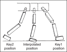
Figure 35.16: An interpolated leg position between key poses found by one of the earliest inverse kinematics algorithms. (Courtesy of A.A. Maciejewski, ©1985 ACM, Inc. Reprinted by permission.)
It is also often desirable to insert a previously authored animation into a novel scene with minor adjustment; for example, to adapt a walk animation recorded on a flat floor to a character that is ascending a flight of stairs without the feet penetrating the ground or the character losing balance. This is especially the case for video games, where the character’s motion is a combination of user input, external forces, and preauthored content [MZS09, AFO05, AdSP07, WZ10].
As we said earlier, motion planning is an AI problem. But it is closely coupled with dynamics. Getting dressed in the morning is more complex than reaching for a book—it cannot be satisfied by a single pose. Presented with a dresser full of clothing, a virtual human would have to not only find the series of poses required to step into a pair of pants while remaining balanced, but also realize that the drawers must be opened before the clothes could be taken out. Figure 35.17 shows some examples of “simple” daily tasks that represent complex planning challenges for virtual characters.
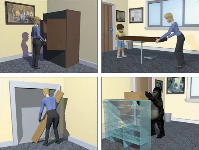
Figure 35.17: Four images of animated characters autonomously performing complex tasks requiring motion planning. (Courtesy of the Graphics Lab at Carnegie Mellon University. ©2004 ACM, Inc. Reprinted by permission.)
A special case of motion planning is the task of navigating through a virtual world. At a high level, this is simply pathfinding for a single character. When there are enough characters to form a crowd, the multiple-character planning problem is more challenging. Creating the phenomenon of real crowds (or herds, or flocks ...) is surprisingly similar to simulating a fluid at the particle level, with global behavior emerging from local rules as shown in Figure 35.18.
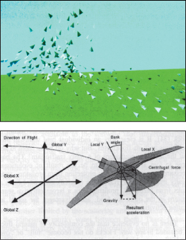
Figure 35.18: Complex global flocking behaviors (top) emerge in Reynolds’s seminal “boids” animation system [Rey87] from simple, local rules for each virtual bird (bottom). (©1987 ACM, Inc. Included here by permission.) (Courtesy of Craig Reynolds, ©1987 ACM, Inc. Reprinted by permission.)
When the space to be traversed does not admit a character’s default method of locomotion, the pathfinding problem is of course much harder. For example, the character in Figure 35.19 must not only find a path, but also decide when to crouch and when to jump to avoid obstacles on the desired path while satisfying physical constraints on the body.

Figure 35.19: A complex traversal requiring both pathfinding and general motion planning [SH07]. (Courtesy of Jessica Hodgins and Alla Safonova ©2007 ACM, Inc. Reprinted by permission.)
Secondary motion is the motion of small parts of a figure relative to its root motion; for example, the flowing of cloth and hair and the jiggling of muscle and fat. Secondary motion is important to our perception of motion and performance, but it is often inefficient to simulate as part of the entire system or explicitly pose. Animators often develop special-case secondary motion simulators that create the character of the motion detail without the full cost [PH06, BBO+09, JP02]. This is analogous to modeling small-scale visual detail in texture instead of geometry.
It is often desirable to transfer an animation performance that was authored or captured on one body to another body [BVGP09, SP04, BCWG09, BLB+08]. There are some cases where there is little choice but to transfer motion between bodies. For example, to animate a centaur with motion capture, we must transfer the motion from a human and a horse onto a single virtual creature. In other cases, it is a matter of cost. Rather than recording the performance of actors of many sizes wearing many costumes, with transfer we could record a single actor and adapt the performance to multiple characters in a crowd [LBJK09].
Plausible animation is the problem of working backward to compute the start state of a system, given the end state [BHW96, KKA05, YRPF09, CF00, TJ07, MTPS04]. For example, a film shot may require a player to roll two sixes on a pair of dice. We would like to start with the sixes facing up at the end of the shot, and solve backward for a physically viable series of bounces as the dice roll that leads them to that position. Since the problem may be overconstrained, we are willing to accept any “plausible” solution in which the laws of physics are bent only in ways that are imperceptible to the average observer. It is plausible for the momentum of a die to be exaggerated by 5% to produce one extra tumble, but not for the die to bounce three meters in the air off the initial throw.
35.5. Pose Interpolation
35.5.1. Vertex Animation
The most straightforward way to represent poses is to specify a separate mesh for each key frame. The mesh topology is usually constant over the animation so that every key frame contains the same number of vertices. Only their positions change, not their adjacency and ordering. To simplify the discussion, assume that key poses k[t] are defined at the ends of integers at time intervals, and that we want to form a continuous expression for the pose at the fractional times t in between these poses.
Sample-and-hold interpolation,
produces substantial temporal aliasing. The character simply holds its position until the end of the time period and then instantaneously snaps to the next pose. This also produces infinite velocity at the frame intervals because x(t) is discontinuous.
We’d like to make smoother transitions with finite velocities. As we said in the introduction, one solution is to linearly interpolate between key poses, which produces continuous positions but discontinuous velocity. That is, we’ve ensured C0 continuity but still exhibit infinite acceleration, which is unnatural for character motion. A higher-order interpolation scheme can produce smoother interpolation. This is a progression that we’ve seen before, when discussing splines in Chapter 22.
Splines are in fact a common solution to the problem of interpolating between key poses. Fitting one Catmull-Rom spline per vertex produces globally smooth animation. Vertex-position splines do not address all of the key pose problems, however. They still require storage proportional to the product of the vertex count and the number of key poses and require a number of interpolation operations linear in the vertex count at runtime. Vertex splines require an artist to pose individual vertices instead of working with higher-level primitives like limbs. Furthermore, the results can be hard to control.
Because each vertex is animated independently and the vertices are only on the surface of the character, there are no constraints to preserve volume or surface area during animation.
35.5.2. Root Frame Motion
Object geometry and vertex animation is typically expressed relative to the root frame of the object. This means that a walking character will stay at the origin while its feet swing below the center of mass. To make the character move around the world we could create an animation in which the vertices all travel away from that starting position; however, this would require a tremendous amount of redundant animation data. Instead, one typically models the transformation of the object root. Root transformations are useful for more than just visible objects in the virtual world. Lights, cameras, 3D widgets, and pointers all define their own frames which may be subject to motion. Throughout this book, we’ve constantly worked with transformations between reference frames, and we’ve seen several alternative representations of a 3D reference frame in Chapters 6, 11, and 12:
• 4 × 4 matrix
• 3 × 3 rotation matrix and translation vector
• Euler angles: roll, yaw, pitch, and translation vector
• Rotation axis, rotation angle, and translation vector
• Unit quaternion and translation vector
In rendering, the 4 × 4 matrix representation is often convenient and is what most APIs have adopted. Because conversions exist between all of these representations, the animation system need not use the same representation as the rendering system. Although the matrix representation is sometimes convenient, the quaternion-plus-vector representation is often preferred for simulation during animation and the Euler frame for motion specification of animation.
When choosing a representation, one typically seeks to minimize error and simplify computations—both for performance and for readability. In animation, we’ll interpolate, differentiate, and integrate expressions containing the reference frames. For a rotating body, performing those operations on the inherently linear matrix structure will typically send points along the tangent to the desired sphere of motion. For small steps, we can correct that error by projecting back onto the sphere of motion, but small steps are not always possible or efficient. Although not without their own problems, the quaternion and angle formulations are better suited to expressing operations on the surface of a sphere. Among these, the axis-angle representation presents something of the same problem as the matrix.
The axis itself must rotate to describe rotations in other planes, and the axis is a linear representation. Euler angles prefer the arbitrary axes chosen (i.e., the magnitude of the derivatives depends on the direction of rotation) and allow gimbal lock under successive 90° rotations. The uniformity of the quaternion therefore leaves it as the best choice in many cases, particularly for freely moving bodies.
Now consider the problem of specifying an object’s motion or the forces that inspire that motion. We often want to choose the reference frame within which it is easiest to create this specification. For many objects, a suitably chosen Euler frame is ideal. For example, an automobile’s front wheels rotate about exactly two axes relative to the car frame. An airplane’s controls affect yaw, roll, and pitch in its own reference frame.
Once the root frame has been transformed, the rigid or dynamic body attached to it can also be moved by simply transforming all of the vertices from the root frame to the world frame. Note that although it is common to place the root frame’s origin within the body (and often at the center of mass), this is just a reference frame, and its origin can lie outside the geometry itself.
35.5.3. Articulated Body
Many objects that we would like to model as a single scene element change their shape as well as their root position and orientation. Some of these objects can be modeled as a collection of bodies that are individually rigid but which transform relative to one another. For example, an automobile can be modeled as a rigid frame and four rigid wheels that rotate relative to the frame. Each vertex in the automobile is contained within exactly one of the bodies, and can therefore be expressed relative to one body’s frame.
A natural way of organizing the bodies relative to one another is a small “scene graph” subtree (see Chapter 6). There is some root body, whose children are other bodies in its frame and the vertices defining the shape of the root body. The other bodies recursively have their own children. In the case of the automobile, it would be natural to choose the car’s frame as the root body. However, a nice property of a tree is that any node can be chosen as the root and the result is still a tree. So we could choose the front-left wheel to be the root, with the frame as its only child body, and the frame would then have three other wheels as child bodies. That choice would probably make it awkward to express the forces exerted by the drive train on the wheels since the tree has little symmetry, but it is a mathematically valid model of the system.
We call this structure an articulated rigid body because the edges of the scene graph typically correspond to joints in the model. A joint is a constraint on the relative movement of two bodies. For the automobile, these are the axles. For an android they would be the knees, elbows, waist, etc.; for a building they would be the door hinges and grooves within which the windows slide. Geometry is often added to the model to visually depict the physical basis for the constraint. However, the animation joints need have no visual representation or physical analog. Typically one puts the root frame of a body at the joint where it is connected to its parent, since that is the frame in which it is most natural to express the joint’s constraint and forces on the two bodies.
An advantage of the articulated rigid body is that complex dynamic objects, such as most machines, can be represented without vertex animation. This is more efficient in both space and time and much simpler to implement. Except at joints, the representation automatically preserves volume.
The limitation of an articulated rigid body is that motion necessarily appears mechanical because the individual pieces remain rigid. Were we to animate a character in this way, the character would appear robotic instead of humanoid. A more general solution is the articulated body. This maintains a scene graph of reference frames, but performs some other kind of animation, such as keyframe vertex interpolation, on the data within those reference frames. The particular combination of rigid frames with vertex-interpolated key frames was very popular for real-time applications like games until fairly recently, when it was overtaken by the more general scheme of skeletal animation.
35.5.4. Skeletal Animation
The shape of the surface of a living creature under motion is dictated by the dynamic position of its skeleton and the constraints of its musculature and other internals. It is sensible to consider parameterizing virtual objects that model such creatures in a similar way. (This is an example of the Wise Modeling principle that says that you should decide what phenomena you want to model, and then be sure your model is rich enough to represent those phenomena.) This is known as a skeletal animation (a.k.a. matrix skinning) model.
A skeletal animation model defines a set of reference frames called bones. That is evocative but something of a misnomer, because reference frames correspond most closely to the joints of the character, not the bones between those joints. The bones may be in a common object space or arranged hierarchically into a tree with parent-child relationships.
We are used to expressing a point as a weighted combination of axis vectors in some reference frame. A single vertex in a skeletal animation mesh is a weighted combination of points in multiple reference frames. For example, a point near a human’s elbow may be defined as halfway between a point defined in the shoulder/upper arm’s reference frame and a point defined in the elbow/forearm’s reference frame. This joint parameterization allows that vertex and its similarly defined neighbors to define a smoothly deforming mesh near the elbow as it bends. That is in contrast to the sharp intersection of surfaces defined in different reference frames observed under articulated rigid body animation.
We can think of a point x represented as a linear combination of specific points Pb transformed by corresponding bone transformation matrices Bb at given times under various scalar weights wb:
where Σwb = 1. However, since Pb and wb are both part of the parameterization that we will compute from an artist’s input and all relevant operators are linear, in practice we need only store 3-vectors ![]() .
.
One typically constructs the representation by having an artist place a skeleton inside a mesh that is in some standard pose. The artist then assigns bone weights to each vertex and the system computes ![]() for each vertex from them. A first approximation might be that each vertex has a single nonzero weight, which is for its position in the standard pose relative to the closest reference frame. The artist then manipulates the skeleton to create a different pose and the vertices transform accordingly. Those near joints are likely to land in undesirable positions, so the artist moves them to the desired position. The system can then recompute a set of
for each vertex from them. A first approximation might be that each vertex has a single nonzero weight, which is for its position in the standard pose relative to the closest reference frame. The artist then manipulates the skeleton to create a different pose and the vertices transform accordingly. Those near joints are likely to land in undesirable positions, so the artist moves them to the desired position. The system can then recompute a set of ![]() values that minimize the position representation error under both inputs. The artist then repeats the process for more poses. Since this quickly becomes an overconstrained optimization process, the resultant weights might not satisfy the visual goal sufficiently in any pose. The artist can reduce the constraints on the system by adding more bones. Often this process results in a majority of bones with no physical interpretation in the original creature—they are present merely to offer enough degrees of freedom for the optimizer to satisfy each of the desired pose deformations. Since the bones need not have a true skeletal correspondence, skeletal animation can also be applied to objects like trees or even water that has no proper skeleton but which exhibits smooth deforming animation.
values that minimize the position representation error under both inputs. The artist then repeats the process for more poses. Since this quickly becomes an overconstrained optimization process, the resultant weights might not satisfy the visual goal sufficiently in any pose. The artist can reduce the constraints on the system by adding more bones. Often this process results in a majority of bones with no physical interpretation in the original creature—they are present merely to offer enough degrees of freedom for the optimizer to satisfy each of the desired pose deformations. Since the bones need not have a true skeletal correspondence, skeletal animation can also be applied to objects like trees or even water that has no proper skeleton but which exhibits smooth deforming animation.
Learning to intuitively introduce new “bones” to yield the desired result from a nonlinear optimizer is difficult. This is one of the reasons that skilled rigging animators are in great demand. Just as we can ease the difficulty of approximating arbitrary shapes with a mesh by increasing the tessellation, we can ease the challenge of rigging a skeleton by increasing the number of bones available. The drawbacks of doing so follow from that analogy as well. At animation creation time (versus model rigging time), each bone must be positioned for each key frame. The number of bones obviously increases the difficulty and time cost of animation. At runtime, the system must transform each vertex. The summation for a single vertex in Equation 35.15 need only be performed for each matrix corresponding to a nonzero weight. Yet even if there are as few as three bones affecting each vertex, that transformation will be three times as expensive as for a rigid body with a single transformation, and the vertices must be batched into small (inefficient) groups that share the same subset of bone matrices versus large uniform streams that are more amenable to efficient processing on parallel architectures.
35.6. Dynamics
35.6.1. Particle
In dynamics, a particle is an infinitesimal body. At human scale, a particle is a reasonable approximation for a molecule, or a grain of sand. At astronomical scale, planets and moons can be modeled as particles. We study particles for two reasons. First, particles and particle systems are frequently used in graphics to model either very small objects, such as bullets, or amorphous compressible objects, such as smoke, rain, and fire [Ree83]. The second reason that we study particles is that they provide a simple system in which to derive dynamics. After deriving the dynamics of a particle we will then generalize to more complex bodies.
Although the particles are infinitesimal, we might still choose to render them as with geometry or billboards. This improves their appearance (a zero-volume particle wouldn’t be visible!) and gives the impression of more complexity than is actually being simulated.
Given the initial position of a particle, its initial velocity, and an expression for its acceleration over time, we want an expression for its position at a later time. Let the unknown position function be t ![]() x(t), where the known initial position is x(0). Recall that x(0) denotes a vector in 3-space. Particles are modeled as points, so we can ignore rotation. This simplifies the physics. Furthermore, for translation, we can treat each axis independently, with two exceptions related to contact: For collisions, objects must overlap along all axes (e.g., at noon on the equator you and the sun have the same xz-position in your local reference frame, but are separated by a huge vertical distance, so you aren’t inside the sun); and for contact force, we need the normal components from all axes to compute the force along each one. For the moment we ignore contact.
x(t), where the known initial position is x(0). Recall that x(0) denotes a vector in 3-space. Particles are modeled as points, so we can ignore rotation. This simplifies the physics. Furthermore, for translation, we can treat each axis independently, with two exceptions related to contact: For collisions, objects must overlap along all axes (e.g., at noon on the equator you and the sun have the same xz-position in your local reference frame, but are separated by a huge vertical distance, so you aren’t inside the sun); and for contact force, we need the normal components from all axes to compute the force along each one. For the moment we ignore contact.
Velocity is change in position divided by change in time. When we say “velocity” we typically are referring to instantaneous velocity ![]() (t), which is the limit of velocity as the time duration approaches zero:
(t), which is the limit of velocity as the time duration approaches zero:
Acceleration has the same relationship to velocity as velocity has to position. Instantaneous acceleration can therefore be expressed as the second time derivative of position:
In this notation, our problem is thus to derive an expression for x(t) given x(0), ![]() (0), and
(0), and ![]() (t). By the second fundamental theorem of calculus, if x(t) is differentiable, then
(t). By the second fundamental theorem of calculus, if x(t) is differentiable, then
Since we have the first and second derivatives of x(t), we will assume that it is in fact a differentiable function.
We cannot apply Equation 35.18 directly because we have no explicit expression for ![]() (t) in our initial state. Therefore, we apply the second fundamental theorem again to obtain an expression in terms of only known values:
(t) in our initial state. Therefore, we apply the second fundamental theorem again to obtain an expression in terms of only known values:
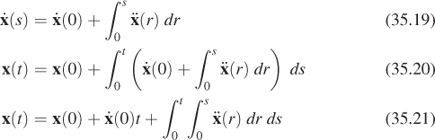
One way to produce a dynamics animation is to evaluate this integral for x(t) analytically and then evaluate it at successive times t = {0, Δt, 2Δt, ...}. When an expression is available for ![]() (t) and it is integrable in elementary (symbolic) terms, this approach is convenient and produces no incremental position error throughout the animation. The analytic approach is viable for simple scenarios, such as a body falling or sliding under constant linear acceleration or a satellite orbiting a planet under constant radial acceleration (both examples due to gravity). Introductory physics textbooks focus on such problems because most complicated scenarios cannot be solved analytically.
(t) and it is integrable in elementary (symbolic) terms, this approach is convenient and produces no incremental position error throughout the animation. The analytic approach is viable for simple scenarios, such as a body falling or sliding under constant linear acceleration or a satellite orbiting a planet under constant radial acceleration (both examples due to gravity). Introductory physics textbooks focus on such problems because most complicated scenarios cannot be solved analytically.
35.6.2. Differential Equation Formulation
Often we have the means to compute instantaneous acceleration given the position and velocity of an object, but no analytic solution for all time. For example, by Newton’s second law (F = m · a), the net acceleration ![]() (t) experienced by a body is the net force applied to it, divided by its mass. The force can often be computed from the current position and velocity of the particle, so given values x(t) and
(t) experienced by a body is the net force applied to it, divided by its mass. The force can often be computed from the current position and velocity of the particle, so given values x(t) and ![]() (t), we could compute
(t), we could compute
for a particle of known mass m and force function f at any possible time t. (Exceptions arise in situations where the force is controlled by user input, for example.)
Equation 35.22 is a (vector) differential equation because it relates x and its derivatives. It is specifically an ordinary differential equation (ODE) because x is a function of a single variable, t. Because f is arbitrary, this happens to be a nonlinear differential equation, which is a hard class to solve. In fact, there is no known analytic solution for general equations of this form.
Introducing an acceleration function does not immediately help us. That’s because we started with the problem that we didn’t have analytic solutions for x and ![]() for all time. Introducing a new function that depends on the two functions we don’t know (and which can’t be evaluated analytically) seems like we’re going in the wrong direction. The key idea here is that if we had values of the functions at a single time, we could compute the forces and thus the acceleration that will help advance the simulation toward a future time without explicitly knowing exactly where it is headed. This will lead us to a numeric integration strategy. This is an important point that underlies most dynamics algorithms. Let us consider a concrete example.
for all time. Introducing a new function that depends on the two functions we don’t know (and which can’t be evaluated analytically) seems like we’re going in the wrong direction. The key idea here is that if we had values of the functions at a single time, we could compute the forces and thus the acceleration that will help advance the simulation toward a future time without explicitly knowing exactly where it is headed. This will lead us to a numeric integration strategy. This is an important point that underlies most dynamics algorithms. Let us consider a concrete example.
Consider a 1D system of a single falling ball whose height is given by height x(t) relative to the ground. Following the notation introduced in Chapter 7, we can explicitly give the type of this function:
(which we might implement in C as float x(float t);, but again, this is a function that we’ll assume we don’t actually have an explicit implementation for).
Likewise, the force function f is
(which we might implement in C as float f(float t, float y, float v); and for which we are assuming the implementation exists).
The function f computes the force on a ball at time t if the ball currently has height y and velocity v. We might model this force as gravity on the Earth’s surface:
Note that under this model f is constant. It doesn’t depend on time, position, or velocity.
A more realistic model accounts for the fact that as the ball moves faster, it experiences more friction with the surrounding air. This drag force inhibits the ball’s motion. That is, it decelerates the ball along the velocity vector. Choosing an arbitrary drag coefficient, we might enhance our model to
Under this new force model, the force on a ball with velocity v = 0 m/s is –9.81 kg · m/s2, while the force on a ball that is already falling with velocity v = –2 m/s has lower magnitude: –8.81 kg · m/s2. This new force model still does not depend on time or position. But we could imagine a more sophisticated model that includes air currents, whose effects depend on the location in space time at which the current is experienced.
Now, consider the ball moving in three spatial dimensions. How do the types of the functions change? Positions and velocities are now 3-vectors:
The force function still takes three arguments. Because it is always applied to position and velocity, people sometimes write f(t, x, ![]() ), treating the x and
), treating the x and ![]() functions as if they were variables.2 Recall the pitfalls of that notation identified earlier in the chapter. So, although you may see that as a convenience in animation notes and research papers, we will continue to be careful to distinguish the function and its value here.
functions as if they were variables.2 Recall the pitfalls of that notation identified earlier in the chapter. So, although you may see that as a convenience in animation notes and research papers, we will continue to be careful to distinguish the function and its value here.
2. We could make this notation meaningful by redefining force as a higher-order function, f : R × (R ![]() R3) × (R
R3) × (R ![]() R3)
R3) ![]() R3, but contorting ourselves to make the notation consistent is not useful because in practice we will apply force function to points and velocities from the previous frame, not functions over all time.
R3, but contorting ourselves to make the notation consistent is not useful because in practice we will apply force function to points and velocities from the previous frame, not functions over all time.
35.6.3. Piecewise-Constant Approximation
Assume for the moment that the force function is constant with respect to time, and that acceleration is therefore also constant. In a physics textbook on Newtonian mechanics, the final position of a body experiencing constant acceleration would be expressed as
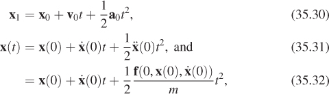
where the second version follows our notation. The right side is quadratic in t and all other factors are constant, so this describes a parabola. That is the arc of a thrown ball, which experiences essentially constant acceleration due to gravity, so this matches our intuition for the position of an object as a function of time. These equations arise from integrating Equation 35.21 under the constant acceleration assumption:
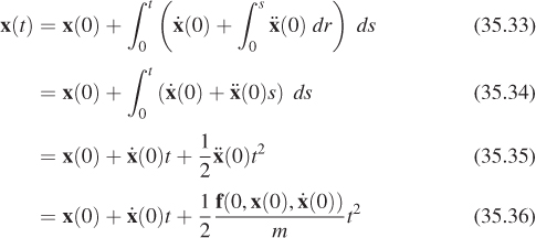
Thus far, we haven’t advanced over the original analytic solution, since we could always evaluate the integral when acceleration is constant. But we can now generalize this result. Assume that f is only constant for each time interval from ti to ti+1 of duration Δt, but may change between intervals. Acceleration is now only piecewise constant over time, which is a much better approximation of the real world.
Under this assumption, we can rework Equation 35.36 to advance a known state described by x(t1) and ![]() (t1) at the beginning of the time interval to the state at the end of the time interval under constant acceleration:
(t1) at the beginning of the time interval to the state at the end of the time interval under constant acceleration:
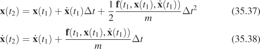
(for constant force on the interval). This is Heun-Euler integration, also known as Heun integration or Improved Euler integration (it is distinct from just “Euler” integration, described in Section 35.6.7.1).
Nothing in these equations assumes a specific number of spatial dimensions, so they hold equally well for the common cases of 1D, 2D, or 3D particles. In fact, we can generalize even further. Rather than limiting x to describing the motion of a single particle, we can pack the positions of multiple particles into x(t) by simply treating them as separate dimensions. We’ll later generalize this even further and encode orientation for bodies with volume in the same vector.
This integration scheme is by no means perfect, but it is often good enough. If the animation doesn’t look right or is unstable, you can often reduce the time interval and the quality will improve. This is because in the limit as Δt ![]() 0 s the Heun-Euler’s estimate approaches the true integral of any arbitrary (integrable) force function. For systems with large or high-frequency forces, you may have to make Δt so small to ensure stability that the simulation becomes quite computationally intense. Section 35.6.6 discusses integration schemes that are more efficient than Heun-Euler for such scenarios.
0 s the Heun-Euler’s estimate approaches the true integral of any arbitrary (integrable) force function. For systems with large or high-frequency forces, you may have to make Δt so small to ensure stability that the simulation becomes quite computationally intense. Section 35.6.6 discusses integration schemes that are more efficient than Heun-Euler for such scenarios.
35.6.4. Models of Common Forces
There are fundamental and derived forces. Fundamental forces such as gravity and electrical force are the elements of the standard physics model and cannot be simplified to the interaction of other forces under that model. Derived forces such as buoyancy are a method for abstracting many microscopic forces into a simple high-level model for macroscopic behavior.
Recall that the net force on a system is written f(t, y, v). If we were considering a single body, then it would have its center of mass be at point y and linear velocity v. In terms of our position function x, we can and often will apply the force function as f(t, x(t), ![]() (t)). As previously discussed, we make the position and velocity explicit arguments distinct from x because that is the form of the function when incorporated into a dynamics solving system.
(t)). As previously discussed, we make the position and velocity explicit arguments distinct from x because that is the form of the function when incorporated into a dynamics solving system.
Forces always arise between a pair of objects. By Newton’s third law of motion, both objects in the pair experience the force with the same magnitude but in opposing directions. Thus, it is sufficient to describe a model of the force on one object in the pair. Likewise, one need only explicitly compute the force on one object in the pair when implementing a simulator. In a system with multiple bodies, the y and v arguments are in arrays of vectors, and the net force function f computes the force on all objects, due to all objects.
For n bodies, there are O(n2) pairs to consider. Forces combine by superposition, so the net force on object 1 is the sum of the forces from all other objects on object 1. This means that the general force implementation of the force function looks like Listing 35.2, where the pairwise force ![]()
(t, y, v, i, j) function computes the force on the object with index i due to the object with index j. There will be many kinds of forces, such as gravity and friction, so we consider an array of numForces instances of ![]() .
.
Listing 35.2: Naive implementation of the net force function.
1 // Net force on all objects
2 Vector3[n] f(float t, Vector3[n] y, Vector3[n] v) {
3 Vector3[n] net;
4
5 // for each pair of objects
6 for (int i = 0; i < n; ++i) {
7 for (int j = i + 1; j < n; ++j) {
8
9 // for each kind of force
10 for (int k = 0; k < numForces; ++k) {
11 Vector3 fi = F [k](t, y, v, i, j);
12 Vector3 fj = -fi;
13 net[i] += fi;
14 net[j] += fj;
15 }
16
17 }
18 }
19
20 return net;
21 }
One would rarely implement the net and pairwise force functions this generally. In practice many forces can be trivially determined to be zero for a pair. For example, the spring force between two objects that are not connected by a spring is zero, gravity near the Earth’s surface can be modeled without an explicit ball model of the Earth, and gravity is negligible between most objects. Other forces only apply when objects are near each other, which can be determined efficiently using a spatial data structure (see Chapter 37). Many of the pairwise force functions don’t require all of their parameters. Taking these ideas into account, an efficient implementation of the net force function for a system with a known set of kinds of forces would look something like Listing 35.3.
Listing 35.3: Specialized net force function.
1 // Net force on all objects
2 Vector3[n] f(float t, Vector3[n] y, Vector3[n] v) {
3 Vector3[n] net;
4
5 // for each object
6 for (int i = 0; i < n; ++i) {
7 net[i] += ![]() gravity(i) +
gravity(i) + ![]() buoyancy (t, y, i);
buoyancy (t, y, i);
8
9 for (int j in objectsNeariWithHigherIndex(i, y)) {
10 Vector3 fi = ![]() friction (t, y, v, i, j) +
friction (t, y, v, i, j) + ![]() normal (y, i, j);
normal (y, i, j);
11 Vector3 fj = -fi;
12 net[i] += fi;
13 net[j] += fj;
14 }
15 }
16
17 // for each pair connected by a spring
18 for (int s = 0; s < numSprings; ++s) {
19 int i = spring[s].index[0];
20 int j = spring[s].index[1];
21 Vector3 fi = ![]() spring (y, v, i, j);
spring (y, v, i, j);
22 Vector3 fj = -fi;
23 net[i] += fi;
24 net[j] += fj;
25 }
26
27 return net;
28 }
Note that we use subscripts to denote the kind of force pair. For example, the force of gravity is denoted ![]() gravity. This is a standard notation in physics, although it is unusual in math. It follows our convention that subscripts denoting meaning (like “gravity” or the “i” and “o” for “incoming” and “outgoing”) are typeset in roman font, while subscripts indicating indexing are treated as variables and typeset in italic. The “gravity” is part of the name of the function, not a variable. In equations we’ll shorten this to just
gravity. This is a standard notation in physics, although it is unusual in math. It follows our convention that subscripts denoting meaning (like “gravity” or the “i” and “o” for “incoming” and “outgoing”) are typeset in roman font, while subscripts indicating indexing are treated as variables and typeset in italic. The “gravity” is part of the name of the function, not a variable. In equations we’ll shorten this to just ![]() g.
g.
Most force functions depend on additional constants that are not explicit arguments. This means that in an actual implementation they would have access to additional information about each object (maybe through applying the provided indices to a global scene array). This is reminiscent of the typical design for a BSDF implementation, where the canonical incoming and outgoing light direction vector arguments are augmented by member variables such as reflectivity and index of refraction.
35.6.4.1. Gravity
Assume that the object with index i is a point mass and that the object with index j is a sphere (or a second point mass). By Newton’s law of universal gravitation, the gravitational force experienced by object i (at yi) due to object j (at yj) is
This remains a good approximation if the radius of the bounding sphere around each object is small compared to the distance between them (e.g., for computing the forces that planets and stars exert on one another).
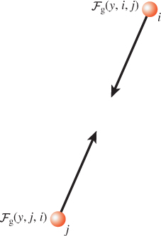
When mj >> mi and the radius of the bounding sphere of object i is small compared to ||yj – yi||, the gravitational acceleration experienced by object i is approximately constant and the gravitational acceleration experienced by object j is negligible. This is the case, for example, when object j is a planet and object i is a human-scale object on the surface of the planet. In this case (Figure 35.21), we can simply ignore j and define the function by
which is a good approximation of gravitational attraction, where g is the acceleration vector. On the surface of the Earth, for example, ||g|| ≈ 9.81m/s2 is a reasonable approximation of the magnitude. The direction is “toward the center of the Earth.” Because it is common to work in a local tangent reference frame on the surface of the Earth that neglects planetary curvature, one often calls that direction “down” and assumes that gravity acts along the constant “vertical” axis.
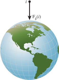
Note that although the gravitational force on an object is proportional to its mass, the acceleration is independent of its mass. This gives rise to the observation that all objects fall at the same pace, neglecting air resistance and other forces. Specifically, the centers of mass of two bodies that experience only gravitational force will fall at the same pace. Individual points on those objects may experience different acceleration and velocity curves. For example, one end of a tumbling stick may actually have a net upward velocity even while the center of the stick is falling.
Gravity is surprisingly weak compared to other forces. A coin-sized refrigerator magnet is able to resist the gravitational attraction of the entire Earth. A human being can temporarily overcome gravity entirely just by jumping. That gravity would be so weak is a puzzling clue as to the nature of the universe, and there is not yet consensus on why it should be this way. For simulation, the weak-gravity observation yields two practical insights. First, we can neglect gravity except in cases of a tremendous size difference between objects or the absence of almost all other forces. For many applications, this generally means we only care about gravitational attraction to the Earth. Second, we can expect most of the forces in a virtual world to have magnitude on the scale of gravity, because they oppose it and keep objects at rest, or to have magnitude substantially stronger than gravity because they move objects despite gravity. This means that tuning the integrator’s constants to be stable for a pile of tumbling blocks is a bad strategy. The force experienced by a rifle bullet when fired or by a car when accelerating can easily be an order of magnitude larger than gravity. Stability should be ensured under the largest anticipated force, which is seldom gravity, and then constants should be tuned for sensitivity so that gravity can still accelerate an unsupported body from rest.
![]() The Structure Principle
The Structure Principle
We can generalize this observation into a Structure principle: Treat surprising structural symmetries and asymmetries as both clues about underlying structure..., and warnings to check the robustness of your plan. For example, if otherwise-similar elements differ by orders of magnitude or demand different parameters, as is the case for the fundamental forces of nature, something interesting is going on that can either lead to insight if followed, or bite you if ignored.
35.6.4.2. Buoyancy
Buoyancy arises from pressure within a fluid medium, such as air or water. It is only observed when the medium and objects within it are exposed to a common external acceleration, such as that due to gravity.
Let vi be3 the volume (in m3) of an object i, ρ the density (kg/m3) of the medium, and g the net gravitational acceleration (m/s2) at the location of the object. Assume that g is constant in the region of interest. Furthermore, assume that both the medium and the object are incompressible, meaning that their volumes do not change significantly under pressure. Water is incompressible, as are many of the things that one might expect to find floating in it, such as wood, buoys, boats, fish, and people.
3. Note that volume vi is distinct from v and ![]() , the variables used for velocity in this chapter.
, the variables used for velocity in this chapter.
If object i is not in the medium, the buoyancy force that it experiences is obviously ![]() b(x, i) = 0 N. If it is submerged (Figure 35.22), then the buoyancy force is
b(x, i) = 0 N. If it is submerged (Figure 35.22), then the buoyancy force is
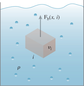
Note that the density of the object does not appear. A dense object will experience less upward acceleration against gravity because of the high force of gravity on the object, not because of a reduction in its buoyancy force. Thus, a “buoyant” object counterintuitively experiences no greater “buoyancy” force than a nonbuoyant one.
The medium of course experiences a force of equal magnitude and opposite direction. However, the medium is by definition a fluid composed of individual freely moving particles, so it is internally a very loosely coupled system. In practice, for animation one often deals with very large bodies of fluid and neglects the impact of buoyancy on them.
For a sense of scale, the density of liquid water is about 1,000 kg/m3 at 4°C, and falls slightly as it is heated or cooled. That this number is exactly a power of ten is no accident—it is one of the constants around which the metric system was originally designed.
Note that the mass and density of the submerged object do not appear. So why do dense objects sink and less dense ones float? Because the net force also depends on gravity: fi = ![]() g(i) +
g(i) + ![]() b. If the object is dense, then
b. If the object is dense, then ![]() g(i) is large compared to
g(i) is large compared to ![]() b and a net downward acceleration is observed.
b and a net downward acceleration is observed.
When the fluid is not at rest, different parts of the fluid exert differing pressure on itself and the objects within it. This leads to wave and vortex phenomena, both at the surface and within the fluid.
35.6.4.3. Springs
Consider an ideal spring that has no mass of its own and that always returns to its rest length after being stretched or compressed and then released. Assume that this spring also only expands and contracts along its “length” axis and is perfectly rigid along axes orthogonal to the length.
Let the spring connect objects i and j (Figure 35.23). Let the spring have rest length r, which means that the spring exerts no force on its ends when ||yi – yj|| = r. By Hooke’s Spring Law, the restorative spring force experienced by object i is
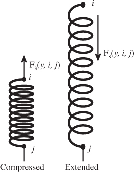
Some springs are stiffer than others. The spring constant ks describes the stiffness of the spring in kg/s2 (this is another case where subscript s is part of the name, not a proper index). Larger constants describe springs that exert higher restorative forces, which we call stiffer, and smaller constants exert smaller forces, which we call softer. When mass is attached to the spring, a stiffer spring will accelerate that mass faster.
Like a pendulum under gravity, a spring will overshoot the rest position and oscillate. Energy lost to friction within the spring or between the mass and air or a surface will cause it to gradually decelerate and come to rest. For some combination of initial conditions and forces the spring could be critically damped so that it exactly comes to rest without oscillating, but the oscillating behavior is more typical. This means that a stiffer spring will not necessarily resume its rest length sooner than a soft one if disturbed—it may merely oscillate with higher frequency, if the frictional forces are too small.
Oscillators under numerical simulation can increase in energy due to roundoff and integration errors, making them unstable. This is exacerbated by the fact that ropes are often simulated as chains of very stiff springs and cloth as networks of stiff springs. Those yield very large forces and high-frequency oscillations, which require very accurate integration to handle stably.
Most springs in the real world lose significant energy due to their own mass and material deformation. It is common to add an explicit damping term to springs to model that loss. This term has the form of a frictional force because it opposes velocity. The damping term has the same form as the original force term, but it applies to velocity instead of position. This means it acts like a “higher order” spring. This makes the problem of tuning springs for stability easier, but does not eliminate it. In the case of a numerical integrator with fixed time steps, an overly large damping constant can actually increase oscillation rather than reducing it when the integral of the acceleration due to damping exceeds the original velocity.
35.6.4.4. Normal Force
An apple on a table experiences a downward force from gravity and negligible downward buoyancy from the surrounding air. Yet the apple is at rest relative to the table, so there must be a force opposing gravity to prevent the apple from experiencing a net downward force. The source of the force is electrostatic repulsion between the molecules of the apple and the table, which keep their surfaces from interpenetrating. We call this a normal force because its axis is perpendicular to the interface between the surfaces. In this case, the interface is the horizontal tabletop, so the force vector experienced by the apple is directed vertically upward along the table’s normal vector. When we consider the case of an object on a tilted surface (Figure 35.24), the normal force is directed away from the surface, but not directly opposing gravity, so it can create a net horizontal acceleration.
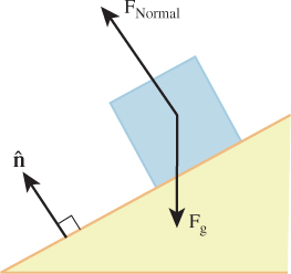
Figure 35.24: The normal force prevents penetration. It is in the direction of the adjacent surface’s normal and has magnitude dependent on all other forces.
The force is trivial to describe but challenging to compute: A normal force is as large as it needs to be to prevent interpenetration of (rigid) objects. It has direction along the normal to the interface and magnitude that is equal to the magnitude of the net sum of all other forces, projected onto that axis.
The normal force is very different from the other forces that we’ve considered. It depends not only on the state of the system, but also on the other forces. For example, when considering spring forces, we can put two masses near each other, attach some springs, and consider their change in velocity and position based solely on the state of the objects. But if we stack ten books on top of a table and ask what the contact forces are between them, then the question doesn’t even make sense. The notion of “compute all of the other forces first” implies an acyclic ordering, which doesn’t exist in this case. Each book within the stack presses both up and down. Therefore, the friction of the normal force breaks down and there are cases where we simply can’t compute reasonable normal forces. Even this simple case of rigid bodies with stacking has proven remarkably challenging—stable, efficient algorithms for solving it were introduced only in the past few years [GBF03, WTF06]. When objects become heavily articulated or have complex contact constraints like the pieces of a completed jigsaw puzzle, simple models like “normal force” break down.
In other words, we’ve changed modes. We have to model something that is outside of our Newtonian model proper, so we’re extending it with a hack. That will be a point where things go wrong. It is ironic that resting contact is surprisingly hard (even before we consider stacking) to simulate compared to the ballistics of a fast-moving bullet. Friction, which relies on normal force, has the same problems. As we discussed in Chapter 1, science depends on the art of modeling what you need for the level of accuracy desired. The simple, first-year Newtonian physics model of normal forces is efficient and accessible, but it is a poor model for complex interactions of many bodies. One can live within those limitations and avoid complex interactions, attempt to patch over the model to hide its failures, or incorporate a more sophisticated model that is probably more expensive to compute and to integrate.
As an example of developing a more sophisticated model, consider that the circular relationships of contact forces are very similar to those studied in light transport. What we need is a steady state solution to an integral equation, and as with light transport there are many mathematical models for numerically approximating that steady state. For this chapter, we will leave this particular problem at that analogy in the interest of returning to efficient simulation of simple systems.
35.6.4.5. Friction and Drag
Friction is a description of a set of forces that lead to the common phenomenon of deceleration. In general, we call any force frictional that is negatively proportional to velocity. This is why friction is described as a force that “opposes motion.” However, “motion” depends on your reference frame.
For example, a car could not move or turn without friction. When a car accelerates linearly, the drive shaft rotates the axles, which then rotate the wheels. Friction between the tires covering the wheels and the road resists the rotation of the wheels. This causes the car to move forward relative to the road, or the road to move backward relative to the car, depending on the reference frame we choose. For ideal tires, this completely eliminates motion in the axis along the road between the point of contact of the tire and the road itself. Thus, friction is indeed opposing some motion. However, there’s little friction perpendicular to the road, so the point of contact is still able to move outside the plane of the road. In this case, it moves upward a moment after it breaks contact. Ignoring deformation, every point on the tire has instantaneous velocity along a tangent to the tire, in the rotational plane of the tire. The tire as a whole is driven by the wheel, the axle, and ultimately the drive train and engine to rotate. Because the point of contact resists motion in the plane of the road, that frictional force propagates backward through the system and produces a net linear acceleration of the car along the road. On ice or in mud there is little friction between a tire and the road. In this case, the points on the tire can move freely relative to the road, so the car does not move.
A similar situation applies to turning a car. At the point of contact, high friction along the axis of the axle resists motion along that axis, while lower friction perpendicular to the axis of the car’s wheel allows motion. This creates a net rotation of the car. Thus, in the broader sense, friction can be essential for enabling motion.
Frictional forces arise from electrostatic repulsion and attraction. In the repulsion case, molecules of adjacent surfaces collide. As we saw when studying BSDFs, surfaces that are macroscopically planar may be microscopically rough. Thus, what appears to be two smooth surfaces sliding parallel to each other may actually more closely resemble the meshed teeth of two long linear gears. This is why rougher surfaces increase friction. It is also why the sole of a new dress shoe is slippery. That sole is a relatively smooth piece of leather. After the shoe has been worn, say, by walking on concrete sidewalks for a few days, the leather sole exhibits small bumps and cracks from uneven wear. These mesh with bumps on the ground and create greater friction.
In the attraction case, materials of different surfaces chemically bond with each other when in contact, and resist being pulled apart. The bonding is often strongest when the two materials are the same. This is why smooth glass slides easily on smooth wood but is hard to drag across another piece of smooth glass (try this with two juice glasses at breakfast!).
There are case-specific models of friction for commonly arising scenarios. We present two here. Dry friction occurs between solids moving parallel to the plane of contact, and drag occurs between a solid and a fluid.
In the dry friction model, the force is factored into static and kinetic (a.k.a. dynamic) terms. Let the two objects be numbered 1 and 2. We consider the force on object 1 in the reference frame the combined system. That is, the center of mass of both objects combined will always be at rest.
Static friction is zero when object 1 is moving, that is, when x(t) ≠ 0 in the system’s frame. When object 1 is still relative to the reference frame of the system and is in contact with object 2 only along a surface, then we model static friction as able to resist acceleration due to net forces up to
parallel to the surface. That is, if the net force is f, then the object will experience no acceleration in the plane of the surface if ||f|| – |f · ![]() | < k. Otherwise, it will experience some acceleration and kinetic friction as described shortly.
| < k. Otherwise, it will experience some acceleration and kinetic friction as described shortly.
The coefficient of static friction μs is determined by the chemical composition of the two surfaces, the amount of surface area in contact, and the microgeometry of the surfaces. In other words, there are a lot of hidden parameters in the static friction equation. However, the coefficient is often approximated as a constant material property in simple simulations.
When two objects already have relative velocity with respect to each other in the plane of their contact, we model kinetic friction. Kinetic friction has lower magnitude than the static friction threshold. This is because objects that are already in motion tend to be bouncing away from their plane of contact at a microscopic scale. Small bounces preclude many of the surface interactions, both chemical and mechanical, that cause friction.
We model kinetic friction (Figure 35.25) as a force
... but we must be careful in simulation to never reverse direction of velocity in a time step due to frictional forces. This constraint must be enforced by the integrator or at least with knowledge of the integrator’s time steps.
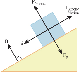
Figure 35.25: Kinetic friction has magnitude proportional to the normal force magnitude and direction opposite velocity (in the plane of the surface).
Drag is the frictional force on a moving object (Figure 35.26) due to the surrounding fluid medium, which is often water or air. Lord Raleigh’s model of drag is a force,
where a is the surface area of the object presented along the direction of motion; Cd is the drag coefficient, which depends on the shape of the object, its roughness, and the chemical composition of the materials; and ρ is the density of the fluid. As with other frictional forces, we must be careful that the drag force does not reverse the direction of motion during a time step.
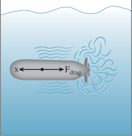
Figure 35.26: Drag forces are caused by friction between an object and the surrounding fluid, and by the pressure built up in the fluid by the object’s relative motion and friction within the fluid. Drag forces are hard to model accurately and efficiently because the fluid’s behavior is complex and highly dependent on the object’s shape at all scales.
Drag force leads to two particularly interesting macroscopic phenomena. The first is terminal velocity. An object falling through a medium does not experience continual net acceleration. For example, a skydiver’s velocity levels off during freefall. This occurs because at some point ![]() g = –
g = –![]() d, since
d, since ![]() d is proportional to velocity but
d is proportional to velocity but ![]() g is constant on the object.
g is constant on the object.
Lift is another interesting phenomenon. An airfoil moving through a fluid experiences a net upward force, which allows airplanes and birds to rise in the absence of updrafts. Bernoulli’s principle describes how lift arises from variations in drag force over the entire surface. As was the case with a car tire, friction is paradoxically enabling motion in this case—just not motion in the direction that the friction opposed.
35.6.4.6. Other Forces
There are of course other fundamental real-world forces: for example, magnetic, strong and weak nuclear, and electrical. These can be adopted from a physics textbook in the same manner as the ones described here. There are also nonfundamental forces that are useful modeling techniques, such as tension and compression, that can be found in any mechanical engineering text.
Nonphysical forces, such as tractor and repulsor beams in a science fiction context, can be described using arbitrary functions. Any force desired can be inserted into the simulation framework, since Newton’s first law of motion reduces it to an acceleration that can be inserted into the integrator.
35.6.5. Particle Collisions
35.6.5.1. Collision Detection
For particles with very small cross sections, collision detection is equivalent to ray tracing. We can ignore the collisions between particles because the probability of those collisions occurring is vanishingly small. The path of a particle over a sufficiently small time interval is a line segment, so by tracing a ray from the particle’s origin in the direction of its velocity we can detect collisions with other parts of the scene. All of the data structures and algorithms built for tracing light rays can thus be applied to dynamics simulation.
It is also possible to model collisions between particles with volume while simulating the movement of each particle as if it were a point mass. To detect a general intersection between two particles we choose the reference frame of one (so that it is not moving), and then extrude the other one along the relative velocity vector. For particles with spherical bounds the intersection test is relatively simple because it is equivalent to testing whether a point is inside a capsule (a cylinder with a hemispherical cap on each end). Collisions between other shapes are often more difficult to compute, and the best solution can be to use a spatial data structure to detect intersecting polygons (see Chapter 37).
35.6.5.2. Normal Forces through Transient Constraints
After a collision is detected, the system must respond to prevent particles from penetrating the scene. We’ve already seen one response—normal forces. When a collision occurs between objects with very low velocity toward each other, it is likely due to resting contact. In this case, reacting to the collision by reversing velocity might introduce energy into the system, since the “collision” itself is an artifact of limited numerical precision for times and positions: Two objects in resting contact should never have accelerated toward each other in the first place. We can restore stability by explicitly moving the objects out of contact or applying normal forces to prevent penetration before it occurs.
We’ve seen that normal forces can be tricky to apply because they must occur “after all other forces” ... which leads to an awkward ordering constraint when normal forces from multiple surfaces are in effect. In systems with a sophisticated integration scheme, it is possible to apply normal forces implicitly rather than explicitly. In these cases, contact creates a temporary “joint” between two objects, requiring that the solution to the simulation during the time step must not move the point of contact on either object [Lö81].
35.6.5.3. Penalty Forces
A generalization of normal forces can elegantly resolve collisions between objects with significant velocities. A penalty force is something like a normal force. It applies to objects that are interpenetrating. The magnitude of a penalty force increases with the level of penetration, and the direction is that which will most quickly separate them. This is actually a reasonable model for microscopic electrostatic repulsion. Atoms never really contact one another. As they come close, they repulse each other with increasing strength until the relative velocities reverse and the proximity decreases. When the force is integrated over the time period from when the penalty force first becomes significant to when it again becomes insignificant, the net result is that of an elastic collision: The velocities of the objects have been reflected about the normal to the plane of their “collision.”
Penalty forces are simple to compute and apply, but often difficult to tune. If the penalty force is too weak, then objects will interpenetrate too far before rebounding. This gives the appearance of overly rubbery materials. If the penalty force is too strong, then any inaccuracy in the integration process can destabilize the system by creating energy due to undersampling. When there are multiple potential points of contact, uneven application of penalty forces due to differing depths of penetration can create a net rotation. With sufficiently large penalty forces this is a further potential for destabilization in the system as small translational error may lead to large rotational error.
35.6.5.4. Impulses
The problem with penalty forces is that they take time to apply, which makes their effectiveness sensitive to the numerical integration scheme of a dynamics simulator. Impulses are an alternative collision resolution strategy that avoids this by directly and instantaneously changing velocities outside of the numerical integration process. This is a good example of the principle of knowing the limits of a model and changing models, rather than patching, when those limits are exceeded.
Numerical integration of forces is stable for constant or slowly varying accelerations, such as those due to gravity, springs, and buoyancy. Numerical integration becomes more fragile for forces with dependency cycles or those that depend on velocity, such as normal and friction forces. For accelerations that vary over time scales shorter than the simulation interval, such as penalty forces, numerical methods generally fail. One approach is to try ever-shorter simulation intervals or more sophisticated integrators, but that is merely shifting the limitation of the model rather than removing it. By pausing numerical integration, directly manipulating velocities with momentum impulses, and then restarting numerical integration, we escape the inherent limitations of integrating derivatives. Note that there is an analogous situation in light transport. In that context, an “impulse” is a spike in a probability distribution function, such as created by a directional light source or a perfect specular reflection. Integrating those zero-area phenomena is just as unstable as integrating a zero-time force. So, stable renderers explicitly handle specular reflections and directional sources with absolute probabilities rather than attempting to make very small angular measurements of very high-magnitude probability distribution functions. In dynamics, we will directly apply velocity changes rather than trying to integrate large-magnitude derivatives of velocity over small-scale time intervals.
Concretely, an instantaneous change means that the integral of acceleration (![]() ) over a zero-second time interval is nonzero; therefore,
) over a zero-second time interval is nonzero; therefore, ![]() is infinite. So we’re applying infinite force for zero time. Specifically, the force and acceleration functions contain mathematical impulses. We can’t directly represent impulses within the integration framework because presenting an infinite acceleration to the numerical integrator will simply result in infinity × 0 = “not a number” under floating-point representations, and because any attempt to perform higher-order integration on such quantities will simply propagate the “not a number” value further. So we step outside the integrator. This of course is a source of instability and error. Anytime the integrator can’t observe a value or control an operation, it becomes vulnerable to roundoff and approximation errors in that operation.
is infinite. So we’re applying infinite force for zero time. Specifically, the force and acceleration functions contain mathematical impulses. We can’t directly represent impulses within the integration framework because presenting an infinite acceleration to the numerical integrator will simply result in infinity × 0 = “not a number” under floating-point representations, and because any attempt to perform higher-order integration on such quantities will simply propagate the “not a number” value further. So we step outside the integrator. This of course is a source of instability and error. Anytime the integrator can’t observe a value or control an operation, it becomes vulnerable to roundoff and approximation errors in that operation.
The impulse equations are derived from the physical concept of linear momentum, which is simply
The change in velocity at a collision will therefore be
The distinction between Δ![]() (t) and
(t) and ![]() (t) is important. We have a rigorous definition of the acceleration function as a derivative:
(t) is important. We have a rigorous definition of the acceleration function as a derivative:
In the presence of an impulse at time t0, ![]() (t) is discontinuous at t0. This means that the lower and upper limits are not equal, so
(t) is discontinuous at t0. This means that the lower and upper limits are not equal, so ![]() (t) is not differentiable at t0. In other words,
(t) is not differentiable at t0. In other words, ![]() (t0) is not defined (which makes sense, since it is “infinite,” yet integrates to a finite quantity).
(t0) is not defined (which makes sense, since it is “infinite,” yet integrates to a finite quantity).
Physicists often employ a Dirac delta “function” δ(t) for which
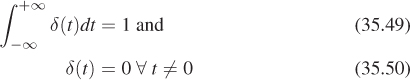
as a notational tool for assigning a value to ![]() (t0) (e.g.,
(t0) (e.g., ![]() (t) = δ(t – t0)Δ
(t) = δ(t – t0)Δ![]() (t)). However, beware that δ(t) is not actually a proper function, and that this notation conceals the fact that differential and integral calculus cannot represent
(t)). However, beware that δ(t) is not actually a proper function, and that this notation conceals the fact that differential and integral calculus cannot represent ![]() (t).
(t).
Since the rest of our simulation is based on numerical integration of estimated derivatives, concealing the facts that ![]() is not differentiable at t0 and
is not differentiable at t0 and ![]() is not integrable at t0 is a dangerous practice. We therefore accept that
is not integrable at t0 is a dangerous practice. We therefore accept that ![]() (t0) does not exist and define a closely related function that does generally exist:
(t0) does not exist and define a closely related function that does generally exist:
where the sign superscripts denote the single-sided limits
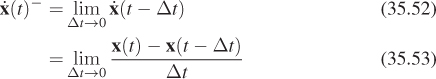
and
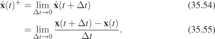
In plain language, a plus sign denotes a value immediately after a collision and a minus sign denotes a value immediately before a collision. The value at the time of the collision is irrelevant, since we’re using the impulse to resolve the collision and jump from the before value to the after value.
The advantage of moving from velocity to momentum is that the law of conservation linear momentum in physics states that the momentum of a closed system is always constant. Therefore,
For a system with exactly two objects whose indices are i and j, the law expands to
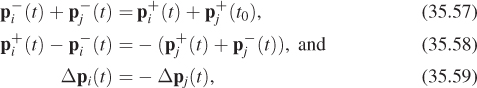
which indicates that we only need to solve for the momentum change of one object explicitly.
Now consider a system with more objects. If we assume that all collisions are pairwise and that exactly one collision occurs at a given time t0, then we can ignore the change in momentum of all objects except i and j and still apply Equation 35.59. This also requires that we be able to assign a strict ordering on multiple collisions. When a simulator encounters a multibody collision the assumption has been violated, and assigning an artificial ordering creates instability. For example, each internal object in a stack continuously collides with two other objects, so it is not surprising that impulse-based simulators often are unstable in the presence of stacked objects.
The linear momentum change in a collision is given by [BW97a]
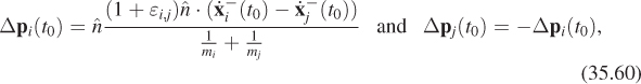
where εi,j is the coefficient of restitution (a measure of how much they resist interpenetration) between objects i and j, ![]() is the unit normal to the contact plane, and m is mass. (Δpi(t0) is often denoted ji.)
is the unit normal to the contact plane, and m is mass. (Δpi(t0) is often denoted ji.)
One nice property of this equation is that it is expressed in terms of inverse masses, rather than masses. This means that the limit of Δp as one of the masses goes to infinity exists and is finite. In practice, it is useful to pin certain objects so that they are not affected by collisions. For example, in a human-scale simulation, simulating the Earth, or even a building as having infinite mass introduces no significant error and typically leads to a simpler implementation of these immovable objects. Beware that assigning infinite mass to a moving object can lead to undesirable behavior, since that object’s momentum is then also infinite. For example, if a train following a prescripted spline strikes a car simulated by dynamics, that car will receive infinite momentum in the collision.
A common model is εi,j = min(εi, εj), where the single-object coefficients are chosen to such that more deformable materials have lower ε. In a perfectly inelastic collision, the objects stick together after collision.
35.6.6. Dynamics as a Differential Equation
![]() Digital computers have limited precision. Therefore, with every iteration of the Heun-Euler Equations 35.37 and 35.38, some error will be introduced. The longer we simulate, the less predictable, and potentially, the less accurate, our solution will be. Of course, unless the forces really were piecewise-constant, approximating them as piecewise-constant is another source of error. Smaller time intervals will lead to finer sampling of the forces and therefore improve accuracy. However, we need many more iterations to span a given time period with small intervals, so there will be more computation and more accumulated error. We now consider numerical methods for solving for x that relax the assumption of piecewise-constant force. These allow fairly large time intervals without undersampling force, which can mitigate the accumulated error problem without increasing the net amount of computation.
Digital computers have limited precision. Therefore, with every iteration of the Heun-Euler Equations 35.37 and 35.38, some error will be introduced. The longer we simulate, the less predictable, and potentially, the less accurate, our solution will be. Of course, unless the forces really were piecewise-constant, approximating them as piecewise-constant is another source of error. Smaller time intervals will lead to finer sampling of the forces and therefore improve accuracy. However, we need many more iterations to span a given time period with small intervals, so there will be more computation and more accumulated error. We now consider numerical methods for solving for x that relax the assumption of piecewise-constant force. These allow fairly large time intervals without undersampling force, which can mitigate the accumulated error problem without increasing the net amount of computation.
Let the function describing the state of the universe at time t be
Although X will be a computationally convenient representation, there is also some physical motivation for it. Both position and velocity (as a proxy for momentum) are included in the state vector because they are properties of objects that appear in mechanical models of the real world. The laws of physics tell us how to compute forces, which are proportional to acceleration. The inputs to force functions are always position and velocity. Forces never turn out to be proportional to acceleration, so we don’t explicitly store acceleration in the state. The exception is the “normal” force model, for which we have already described the problems arising from including acceleration as an input.
Note that X(t) describes the second and third parameters of the f and impulse functions; we can redefine them to take only two parameters and thus write
When considering multiple particles with varying mass, we could replace f/m with f · M–1 for some diagonal matrix of masses M. Note that differential Equation 35.62 is the system version of the single-particle relation previously introduced in Equation 35.22.
Chapter 29 framed light transport in the rendering equation, which was an integral equation. As was the case there, considering general-purpose numeric methods will lead us to broader computer science than needed for the specific dynamics problem at hand. This has two advantages. We can build on previous work that is not graphics-specific, including not just mathematics but also numerical ODE-solving software libraries. We can also take the algorithms that we develop and apply them to other problems beyond dynamics, both in computer graphics and in other fields.
35.6.6.1. Time-State Space
Let’s look at a concrete example to gain some intuition for the 2n + 1-dimensional time-state space defined by t, X(t).
Figure 35.27 shows the path (described by its y-coordinate) of a cannonball that is modeled as a particle in a 1D universe. The upper-left plot shows the familiar time-space path plot of x(t) versus t, which is a parabola. The upper-right plot shows the time-velocity path plot of ![]() (t) versus t, which is linear because the ball experiences constant negative acceleration. This path crosses
(t) versus t, which is linear because the ball experiences constant negative acceleration. This path crosses ![]() (t) = 0 at the apex of the cannonball’s flight. The lower-left image combines these to show the time-state path plot of X(t) versus t. Keep in mind that X describes the entire universe, not just one object. In this example, they happen to be the same because we’re considering a universe with a single particle. Were there more particles, the plot would have many more dimensions.
(t) = 0 at the apex of the cannonball’s flight. The lower-left image combines these to show the time-state path plot of X(t) versus t. Keep in mind that X describes the entire universe, not just one object. In this example, they happen to be the same because we’re considering a universe with a single particle. Were there more particles, the plot would have many more dimensions.
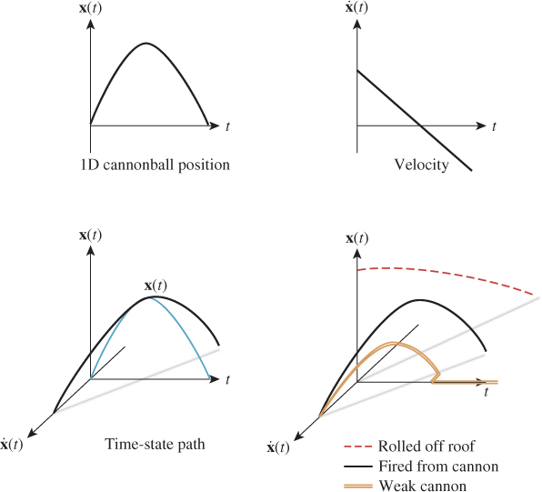
The thick line in the lower-left subfigure shows one particular X of the many that could exist. The thin lines are its projection onto the (t, x)- and (t, ![]() )-planes as “shadows” for reference. Those shadows are exactly the upper-left and upper-right figures.
)-planes as “shadows” for reference. Those shadows are exactly the upper-left and upper-right figures.
From the perspective of t = 0, the dark (t, X(t))-curve describes the entire future fate of the universe. From the perspective of some point at the high end of the timeline, this is the history of the universe. But that curve is only one possible reality. Were there different initial conditions, X would have been a different function and traced a different curve.
The lower-right subfigures depicts three alternative curves that could have been solutions to X, given different initial conditions. Here only the shadows on the (t, ![]() )-plane are shown to keep the diagram simpler. One thick curve is our original cannonball, another is a cannonball rolling off a roof, where
)-plane are shown to keep the diagram simpler. One thick curve is our original cannonball, another is a cannonball rolling off a roof, where ![]() (0) = 0 and x(t) > 0; and the third is a cannonball fired from a weak cannon so that the initial velocity is small but nonzero. That cannonball strikes the ground early and has zero velocity and position after collision. There are infinitely many other solutions for X in Equation 35.62, depending on the initial state.
(0) = 0 and x(t) > 0; and the third is a cannonball fired from a weak cannon so that the initial velocity is small but nonzero. That cannonball strikes the ground early and has zero velocity and position after collision. There are infinitely many other solutions for X in Equation 35.62, depending on the initial state.
By definition, the initial state of the universe is entirely identified by the value that we choose for X(0). There is nothing special about t = 0. Ignoring forces from human interaction, for any particular ti the entire future solution for t > ti is determined by X(ti). In other words, if you give me an X(0), I can tell you X(t) for all subsequent t. My response is a curve in (t, X)-space. If you give me a different X(0), I’ll give you a different curve. Every point lies in space on one of these many possible curves. Furthermore, the curves aren’t merely geometry: They are parametric curves, with parameter t. That is why it makes sense to compute ![]() (t).
(t).
This exercise is mandatory. Don’t progress until you’ve completed it.
We’ve just discussed the initial conditions that give rise to three different (t, X) curves shown in the lower-right subfigure of Figure 35.27. Make a copy by hand of that lower-right subfigure. Think about how we drew the curves and the equations that govern them—don’t just copy the shape.
Now, consider a new scenario. Someone takes the (ill-advised) action of leaning out a window halfway up the building with a cannon, points it straight upward, and fires off a cannonball. Write down the equation of motion as a function X(t) and draw the trajectory in time-state space superimposed on the previous curves.
Consider the tangents to solution curves for t versus X, like those in Figure 35.27. They define some vector field over the time-state space such that if the universe we are simulating has solution X, the value of this vector field is ![]() (t) at (t, X(t)). Formally, let D be the vector-valued function such that
(t) at (t, X(t)). Formally, let D be the vector-valued function such that
In the context of physical simulation under Equation 35.62, this means that
although in the following derivation we will make no assumptions about D, X, or ![]() , so as to keep the discussion valid for all ordinary differential equations. From here on, these will simply be arbitrary functions, which may not even be vector-valued, and our goal is to trace a flow curve through the tangent field.
, so as to keep the discussion valid for all ordinary differential equations. From here on, these will simply be arbitrary functions, which may not even be vector-valued, and our goal is to trace a flow curve through the tangent field.
We chose the letter “D” because the tangent field function is reminiscent of the derivative ![]() . It is not actually the derivative: D is a field over time-state space (as shown in Figure 35.28) and
. It is not actually the derivative: D is a field over time-state space (as shown in Figure 35.28) and ![]() is the tangent function to one particular curve X through that space. That is, every solution X is a flow curve of the field D.
is the tangent function to one particular curve X through that space. That is, every solution X is a flow curve of the field D.
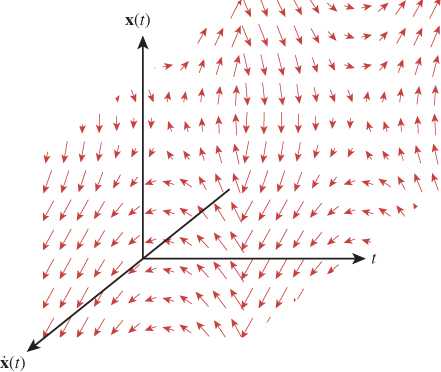
Figure 35.28: Visualization of D for the state space of one 1D particle under some arbitrary forces.
If we were following a particular solution X and somehow stepped off that curve, the D field would guide us along some other flow curve that quite likely diverged from our original solution. Figure 35.29 depicts two instances of this situation for a simple tangent field. Although it is undesirable, this will prove to be unavoidable during our numerical evaluation, and the best that we can do is to try to minimize divergence and encourage transitions that are at least plausible.
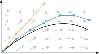
Figure 35.29: A flow curve through a tangent field, and two attempts to follow it in discrete steps.
35.6.6.2. Following the Tangent Field
Consider a series of state vectors {Y1, Y2,...} such that Yi ≈ X(ti), where the sampling period ti+1 – ti = Δt is constant. These are the regularly spaced samples of the state function X that we want the simulation system to provide.
To find these, we begin with an exact initial state Y1 = X(t1). We want to follow the flow curve of D that passes through (t1, Y1) until it intersects the plane t = t2. That intersection is at Y2. We then repeat the process for every other sample. This strategy evaluates X by numerical integration of the ![]() function implicit in D, rather than solving for an explicit expression for X or
function implicit in D, rather than solving for an explicit expression for X or ![]() .
.
The process is a little like a detective tailing a suspect in a black sedan in city traffic. The detective doesn’t want to be observed. So he stays a few cars behind on the road, out of the suspect’s line of sight. But he also doesn’t want to lose the suspect, so he has to periodically pull up closer to catch sight of the sedan. Here, the sedan’s path is the solution X that we (and the detective) want to follow, and checking the location of the sedan is like evaluating D. The detective’s actual path is defined by the Y values, which we want to follow X, but might diverge if he isn’t careful. Unfortunately for our detective, there are a lot of other black sedans on the road that don’t contain the suspect—and for our dynamics solver there are other solutions to X that don’t match our initial conditions. If the detective waits too long between checking on his suspect, he might accidentally start following the wrong sedan. In the equivalent situation, our solver might start tracking the wrong solution.
The previously explored Heun-Euler solver in Equations 35.37 and 35.38 made the assumption that the D field described linear flows over the time intervals. This is like pausing exactly once per time interval, choosing a direction, and then following the parabolic curve that exits our current position in that direction. We could do worse; for example, following a line that exits our current position in that direction. That process is called Explicit Euler integration. We can also do much better than either Heun-Euler or Explicit Euler, in terms of estimator quality versus computation.
To see how, we stretch our car-chase analogy a little further. The detective has more choices than just driving straight toward where he last saw the sedan. He can watch the sedan for a while (i.e., evaluate D at multiple points), and then make an educated guess about where it is really going before dropping back out of sight. We’ll cover strategies for this in Section 35.6.7. First let’s look at how we will employ such a strategy in terms of a general dynamics solver.
35.6.6.3. A General ODE Solver
The framework for the numerical method for evaluating solutions to ODEs at specific time intervals is extremely simple. Function D is implemented as a first-class closure. The mechanism for this depends on the language: a class in C#, C++, or Java, a function in Python, Scheme, or Matlab, and a function pointer and void pointer in C.
The integrator that advances Yi to Yi+1 is shown in Listing 35.4.
Listing 35.4: ODE integrator using Explicit Euler steps.
1 vector<float> integrate
2 (float t,
3 vector<float> Y,
4 float Δt,
5 vector<float> D(float t, vector<float> Y) {
6
7 // Insert your preferred integration scheme on the next line:
8 ΔY = D(t, Y) · Δt
9
10 return Y + ΔY
11 }
We will replace the center line with alternate expressions in what follows. The method shown is the least computationally expensive and least accurate reasonable method for evaluating ΔY.
35.6.7. Numerical Methods for ODEs
![]() There is a tradeoff between the computational cost of a single iteration and the number of iterations required to maintain accuracy. In general, one is willing to perform significantly more work per iteration to take large time steps. However, for graphics applications the time step may be driven by the rendering or user input rate, and therefore there is a limit to how large it can be made. Furthermore, the D function may be very expensive to evaluate because it can include collision detection and a constraint solver. Thus, although for general applications the 4th-order Runge-Kutta scheme is the default choice, many dynamics simulators for real-time computer graphics still rely on simple Euler integration.
There is a tradeoff between the computational cost of a single iteration and the number of iterations required to maintain accuracy. In general, one is willing to perform significantly more work per iteration to take large time steps. However, for graphics applications the time step may be driven by the rendering or user input rate, and therefore there is a limit to how large it can be made. Furthermore, the D function may be very expensive to evaluate because it can include collision detection and a constraint solver. Thus, although for general applications the 4th-order Runge-Kutta scheme is the default choice, many dynamics simulators for real-time computer graphics still rely on simple Euler integration.
The basic idea underlying all of the integration schemes presented in this chapter is that any infinitely differentiable function f can be expressed as the Taylor polynomial,4
4. This is only guaranteed to hold on some neighborhood of t0. In practice, this neighborhood is usually the whole real line (for functions which mathematians call “analytic”), but there exist functions for which the neighborhood is very small. Impulses are one case where the neighborhood is not the entire real line, which gives more intuition as to why they do not interact well with the ODE framework for dynamics.
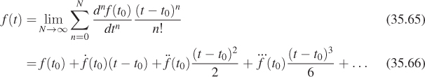
A finite number of Taylor terms allows approximation of f(t) for arbitrary t. To apply this, we must know the value of the function f(t0) at some specific time t0, and some derivatives of f at t0. For the dynamics application of approximating Y ≈ X(t), we know X(t0) because that is the current state of the system. We also know ![]() (t0) because that is the velocity and acceleration, which can be computed by the D function. We can therefore immediately make the two-term approximation:
(t0) because that is the velocity and acceleration, which can be computed by the D function. We can therefore immediately make the two-term approximation:
The highest-order term present in this approximation is the n = 1 term, so this is called a first-order approximation. This particular first-order approximation leads to the integration scheme just presented, and is known as Forward Euler integration.
The error in an approximation of a Taylor polynomial with a finite number of terms is the missing higher-order terms. If the magnitude of higher-order derivatives grows no faster than the factorial, higher-order terms have successively less impact. This is true for many functions encountered in practice, especially physical simulation without impulses. The error in a first-order approximation is therefore dominated by a second-order term. That term contains (t – t0)2, so for a time step Δt = t – t0, it is often referred to as growing like O(Δt2). This is a bit misleading. For large n, the factorial in the denominator decreases the magnitude of the higher-order terms faster than the exponent on Δt. Furthermore, for Δt > 1, Δtn increases with order, and the point at which that occurs depends on the arbitrary choice of units for measuring time (although the derivative also changes to counteract this, as we’ll see in a moment). So a better way to think about the accuracy of an approximation is that an “nth-order approximation” contains n terms of the Taylor expansion.
In a dynamics system we do not have an explicit function for higher-order derivatives of X. However, by applying the definition of the derivative to D, we can estimate higher-order derivatives for specific values of t. For example:
We can approximate the limit by choosing any t > t0, with accuracy typically decreasing at larger time steps. Recursively applying the numerical derivative form allows estimation of arbitrarily high derivatives. Note that the nth derivative contains (t – t0)n in its denominator, which will be canceled by the same coefficient in the numerator of the Taylor polynomial. Thus, many numerical integrators don’t explicitly contain higher powers of the time step in their final form.
The challenge in estimating the numerical derivatives is that we can’t apply the D function at t0 unless we know X(t0). Since we’re trying to solve for X(t0), this means we can’t solve until we already know the solution. Fortunately, we can estimate X(t0) with some (n – 1)th-order method. We can then use that value to numerically estimate an nth-order derivative. To prevent the error from these successive estimations from accumulating, many schemes then go back and reestimate X(t0).
One can estimate arbitrarily high derivatives with arbitrary accuracy by this method. Increasing accuracy in the derivatives allows larger time steps, which allows fewer computations per unit simulation time. However, there is a computational cost for each D evaluation. If the net cost of computing an accurate derivative to take a large time step is higher than that of computing a less accurate derivative and making many small time steps, nothing has been gained. The choice of what order of integrator to apply therefore depends on the cost of D, which depends on the complexity of the scene and forces. This is why there is no single “best” integration scheme for dynamics.
35.6.7.1. Explicit Forward Euler
We’ve already seen the Explicit (a.k.a. Forward) Euler method,
in which Y is the initial state of the system, D is the field for which D(t0, Y) ≈ dY(t0)/dt, and Δt is the duration of the time interval.
This is perhaps the simplest and most intuitive integrator. The change in state of the system is our estimate of the current derivative scaled by the time step. For position, this corresponds to assuming that velocity is constant (i.e., acceleration is zero) and thus advancing by the current velocity. It obviously is a good estimator when those conditions are true and is a worse estimator when there is significant acceleration.
35.6.7.2. Semi-Implicit Euler
Explicit Euler integration only considers the derivative (e.g., velocity) at the beginning of a time step. Under large accelerations, that is a poor estimate for the derivative throughout the time step. An alternative is to use the derivative from the end of the time step. The challenge in doing so is that since we’re trying to estimate the state of the system at the end of the time step, it is hard to use values from that time to reach it.
The Semi-Implicit Euler (confusingly also known as Semi-Explicit Euler) method performs a tentative Explicit Euler step to the end of a time interval and measures the derivative there. It then returns to the beginning of the interval and applies the discovered derivative to the original position. This is more stable than Explicit Euler and much less expensive than the full Implicit Euler method, which requires iterating on this process to find a fixed point [Par07].
Expressed in our state notation, the Semi-Implicit Euler integrator is
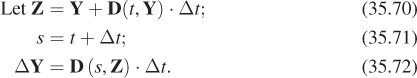
35.6.7.3. Second-Order Runge-Kutta
Runge-Kutta5 refers to a family of related iterative methods for approximating solutions to ODEs. They are described by a set of coefficients and the number of stages, where each stage requires one evaluation of D based on the result of previous evaluations. See [Pre95] for the general form of Runge-Kutta methods.
5. Phonetically: “run-ga cut-a”
Explicit Euler is the only one-stage Runge-Kutta method. A commonly employed one of the many possible two-stage Runge-Kutta methods is
35.6.7.4. Heun
Heun’s method is an improved two-stage Runge-Kutta method compared to the one just presented. It is equivalent to averaging the steps from the Explicit and Semi-Implicit Euler methods, and to the scheme previously presented in Equations 35.37 and 35.38. Heun’s method is also known as the Modified Euler and Explicit Trapezoidal methods.
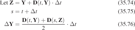
35.6.7.5. Explicit Fourth-Order Runge-Kutta
The classic fourth-order Runge-Kutta method is one of the most commonly used integrators for dynamics in computer graphics and is the most accurate integrator in this chapter. It is:
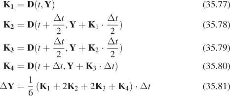
One might always use fourth-order Runge-Kutta, and in fact, that is the approach of many dynamics experts. However, for state configurations in which evaluating D is very expensive, one must consider the net cost of using a better integrator compared to using more and smaller time steps with a worse integrator. We generally care about the wall-clock time to achieve stable integration, and that might be better achieved through taking many small Euler steps. Again we see analogy to light transport: Many inexpensive samples may achieve faster convergence than few expensive samples. Thus, only with an end-to-end convergence, stability, and performance goal can we make a design decision for a particular system.
35.7. Remarks on Stability in Dynamics
While performance and scalability are important, dynamics is one of the few areas in computer graphics where numerical stability, and not performance, is the primary concern and focus of advancement. Numerical stability is related to precision and accuracy, but it is not the same as them. A simulation of a block tumbling down stairs is accurate if it produces results close to those of the corresponding real-world scenario. The simulation is precise if there are many bits in the output (regardless of whether they have the correct values!). The simulation is stable if the block reliably tumbles down, rather than gaining energy and launching into space or exploding, for example. The challenge is that stability is often opposed to accuracy. If the block merely remains sitting at the top of the stairs, even when unbalanced, the simulation is stable but so inaccurate that it is useless. Although stability is often driven by energy conservation, such events as missed collisions, infinite (conserving) spring oscillations, and infinite (conserving) micro-collisions may also be characterized as instability.
Why is stability so difficult to achieve in dynamics? As we’ve seen in this chapter, dynamics is deeply related to ordinary differential equations and numerical integration. A numerical integrator’s precision and accuracy are governed by three elements: its representation precision (e.g., floating-point quaternions), its approximation method for derivatives, and its advancement (stepping and integration) method. Each of these is a complex source of error. When integrating forward in time, the feed-forward nature of the system creates positive feedback that tends to amplify errors. This is what often creates additional energy and is a major cause of instability. Solving via a noncausal process (i.e., looking both forward and backward in time) can counter the positive feedback loop with corresponding negative feedback, which may increase stability. Unfortunately, solving a system for all time generally precludes interactivity, in which future inputs are unknown.
In contrast to dynamics, physical simulation of light transport by various algorithms typically converges to a stable result. Energy in light differs from that in matter in three ways: Photons do not interact with one another (at macroscopic scales, at least), energy strictly decreases at interactions along a transport path through time and space (in everyday scenarios, at least), and the energy of light is independent of its position between interactions. The last point of comparison is the subtlest: Kinetic energy is explicit in a dynamics solver, but potential energy is largely hidden from the integrator and therefore a place in which error easily accumulates.
Thus, although algorithms like radiosity and photon mapping simulate light exclusively forward (or backward) in time, the feedback in the light transport integrator is not amplified by the underlying physics. In contrast, in dynamics, the laws of mechanics and the hidden potential energy repository conspire to amplify error and instability. Even worse, this error is often not proportional to precision, so one’s first efforts at addressing it by increasing precision are often insufficient. For example, turning all 32-bit floating-point values into 64-bit ones or halving the integration time step often doubles simulation cost without “doubling” stability. As a result, many practical dynamics simulators are rife with scene-specific constants controlling bias, energy restitution, and constraint weights. Manual tuning of these constants is tricky and often unsatisfying, since a loss of accuracy is frequently the price of stability.
Thus, instability is an inherent problem in dynamics for interactive systems. Stability is a primary criterion for evaluating dynamics systems and algorithms, and much good work has been done on it in both industry and academia. Looking toward the future, we offer two speculations on stability.
The first speculation is that the structure of the integrator may be at least as important as the schemes it uses for derivatives and steps, and that this may be a fruitful area in which to seek improvements. This statement is motivated by Guendelman, Bridson, and Fedkiw’s work on stability for stacks of rigid bodies [GBF03]. They showed that simply reordering steps in the inner loop of the integrator can dramatically increase stability for scenarios that have been traditionally challenging to simulate, and then demonstrated some additional sorting methods for enhancing stability further. This inspired others to experiment with the integration loop, and has led to various minor changes that produced significant increases in the stability of popular dynamics simulators. This area merits further study.
The second speculation is that the conventional wisdom, “fourth-order Runge-Kutta with fixed time steps is good enough” for dynamics in computer graphics, has not been formally explored. Numerical integration is essential to other fields and is an area of constant scientific advance. We are not aware of experiments with various newer integration methods, particularly adaptive step-size ones, in dynamics simulation for computer graphics. Thus, it is an open question where the best tradeoff lies between per-step cost and steps per frame. Recall that the benefits of higher-order integration are only justified if they result in fewer steps and implicitly conserve precision. Taking more low-order steps, especially on massively parallel processors, could be preferable in some systems. Alternatively, taking very few high-order steps could be preferable. Thus, experimentation with the core numerical integration scheme is another area that may yield interesting results. Our understanding is that physical simulation for nongraphics engineering and science applications has been proceeding in this direction and we encourage its development within graphics as well.
35.8. Discussion
We’ve explained in this chapter how physically based animation can be described by differential equations whose solutions present various challenges, depending on context. The other kind of animation, which one might call “fine-art animation,” and which involves human animators, is a separate discipline. Nonetheless, physically based animation and algorithmic animation are being used more and more, even within fine-art animation. This presents challenges and opportunities in designing comprehensible interfaces for artists who must interact with physics and try to control it to achieve certain artistic goals.