
Chapter 33. Shaders
33.1. Introduction
This chapter is about shaders, pieces of code written in a shading language, a specialized language that’s designed to make shader writing easy. Shaders describe how to process data in the graphics pipeline. Shading languages are evolving so fast (as is the programmability of the pipeline itself) that this chapter will be out of date before its last sentence is written, let alone before you read it. Despite this rapid evolution, there are some things that are invariant across several generations of shading languages, and that we anticipate will remain in future versions for at least a decade. There’s some reason to believe this. The evolution of the graphics libraries that link a program on a CPU to one or more programs on the GPU has been from the specific (in early years) to the general, to the point where much of GL 4 resembles an operating system rather than a graphics library: It’s concerned with linking together executable pieces of programs on the CPU and GPU, passing data between processes, starting and stopping threads of execution, etc. There’s no obvious further generalization that can happen, at least in the near term. Perhaps in five years you’ll write shaders directly in C# rather than in a specialized shading language, and those shaders will run on 500-core machines. But in many ways they’ll continue to look the same: The first thing we usually do with vertex data is to transform it to world-space coordinates using multiplication by some matrix. That will look the same, no matter what the language.
We’ll therefore describe a few shaders, using GL 4 as our reference system, and trusting that you, the reader, will be able to interpret the ideas of this chapter into whatever shading language you’re using.
33.2. The Graphics Pipeline in Several Forms
Figures 33.1 and 33.2 show the various steps involved in either a rasterizing renderer or a ray tracer, as described in Chapter 15.
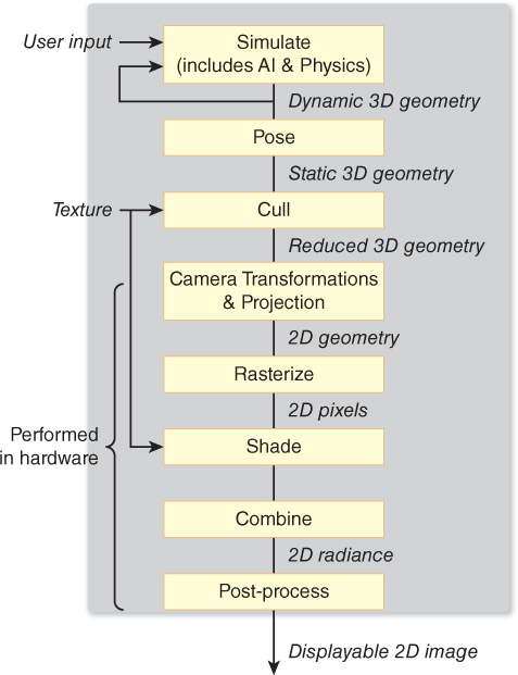
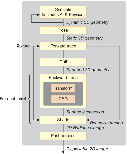
There are many operations—transforming objects from object space to world space to camera space, shading, placing pixel values in a buffer for later use (either in environment mapping, for instance, or in compositing with some other precomputed imagery)—that occur in both pipelines.
As software engineers, we know that when there’s commonality, there’s an opportunity for abstraction and the development of an interface to the common portions of the code. The particular form of the interface can vary: Some designs employ virtual methods, others use callbacks, etc. In some cases the thing being abstracted is complex enough that the way in which it’s used is itself complex. In these cases, it makes sense to create a language in which the use pattern is described via small programs. We’ve seen an example of this with WPF in earlier chapters: XAML provides a language for describing objects, their geometric properties, their relationships, and how data is passed among them, for instance. A C# program usually combines with XAML code to constitute an entire graphics project.
In the case of the graphics pipelines shown in the preceding figures, there’s a common structure: The geometric and material descriptions of objects in a scene undergo similar transformations, for instance, in a similar order in both pipelines. But the details of what goes on at certain stages vary. Shaders are small programs that specify how the duties of certain portions of the pipeline are to be carried out.
The sidebar in this chapter describes informally how we got from individual renderers written in research laboratories to the software design of packages like GL 4.
33.3. Historical Development
Immediate-mode packages like GL in its early forms provided ways to represent, in the sequence of instructions issued to the package (typically by function calls), something about the structure of the objects to be drawn. If an object was modeled with a hierarchy of transformations, then the sequence of GL calls would reflect this, pushing and popping matrix transformations from a stack that represented a current transformation to be applied to all subsequent vertices. These transformed vertices, together with vertex-index triples representing triangles, formed the core of what was to be rendered. The rendering process followed a fairly straightforward path, which can be coarsely summarized by saying that a collection of triangles with per-vertex and per-triangle attributes were described to the system, often with various transformations applied to the vertices. The resultant triangles were then transformed to the standard perspective view volume, and clipped against the near clipping plane. They were then transformed to the standard parallel view volume, and clipped against the remaining clipping planes. The resultant triangles were then rasterized, the rasterized pixels were shaded (i.e., some computation was done to determine their color, a computation that often involved texture lookup), and the triangles were placed into a Z-buffer, with only the front-most remaining in the final image. Sometimes the resultant image was combined with some preexisting image via a compositing operation so that multiple objects could be rendered in separate passes and then a single image could be produced at the end.
As graphics developed, the particular choices of transformations to be applied to triangles, or how values computed at vertices were to be interpolated across triangles, or even how high-level descriptions of objects were to be converted to triangle lists, all varied. But there were a few things that were shared by essentially all programs: vector math, clipping, rasterization, and some amount of per-pixel compositing and blending. The development of GPUs has reflected this—GPUs have become more and more like general-purpose processors, except that (a) vector and matrix operations are well supported, and (b) clipping and rasterization units remain a part of the design. The modern interface to the GPU now consists of one or more small programs that are applied to geometric data (these are called vertex shaders), followed by clipping and rasterization, and one or more small programs that are applied to the “fragments” produced by rasterization, which are called pixel shaders or fragment shaders. A more appropriate name for what’s currently done—computing shading values for one or more samples associated to a pixel—might be sample shaders. The programmer writes these shaders in a separate language, and then tells the GPU in which order to use them, and how to link them together (i.e., how to pass data from one to the other). Typically some packages (like GL 4) provide facilities for describing the linking process, compiling and loading the shaders onto the GPU, and then passing data, in the form of triangle lists, texture maps, etc., to the GPU.
Why are these programs called shaders? In the GL version of the Lambertian lighting model, similar to the one presented in Chapter 6, the color of a point is computed (using GL notation) by
where ![]() is the unit direction vector to the light source, kd is a representation of the reflectance of the material, Cd is the color of the material (i.e., a red-green-blue triple saying how much light the surface reflects in each of these wavelength bands), L is the color of the light (again an RGB triple, which is multiplied term by term with Cd), and n is the surface normal. In Phong lighting, another term, involving the view vector as well, and ks, a specular constant, Cs, a specular color, and ns, the specular exponent, are added.1 Increasingly complex combinations of data like this, including texture data to describe surface color or surface-normal direction, etc., got added, and the formulas for computing the color at a point got to look more and more like general programs. Cook [Coo84] introduced the idea that the user could write a small program as part of the modeling process, and the rendering program could compile this program into something that executed the proper operations. Cook called this programmable shading, although perhaps programmable lighting would be a better term for the process we’ve just described. In that era, the computation entailed by lighting models was often so great that it made sense to do much of the computation on a per-vertex basis, and then interpolate values across triangles; the interpolation process was called shading, and it varied from the interpolation of the colors to the interpolation of values to be used in computing colors. Since papers describing lighting models often also described such shading approaches, the two ideas became conflated, and the term “shader” was used for the new notion.
is the unit direction vector to the light source, kd is a representation of the reflectance of the material, Cd is the color of the material (i.e., a red-green-blue triple saying how much light the surface reflects in each of these wavelength bands), L is the color of the light (again an RGB triple, which is multiplied term by term with Cd), and n is the surface normal. In Phong lighting, another term, involving the view vector as well, and ks, a specular constant, Cs, a specular color, and ns, the specular exponent, are added.1 Increasingly complex combinations of data like this, including texture data to describe surface color or surface-normal direction, etc., got added, and the formulas for computing the color at a point got to look more and more like general programs. Cook [Coo84] introduced the idea that the user could write a small program as part of the modeling process, and the rendering program could compile this program into something that executed the proper operations. Cook called this programmable shading, although perhaps programmable lighting would be a better term for the process we’ve just described. In that era, the computation entailed by lighting models was often so great that it made sense to do much of the computation on a per-vertex basis, and then interpolate values across triangles; the interpolation process was called shading, and it varied from the interpolation of the colors to the interpolation of values to be used in computing colors. Since papers describing lighting models often also described such shading approaches, the two ideas became conflated, and the term “shader” was used for the new notion.
1. In the terminology we’ve used from Chapter 14 onward, these would be the “glossy” constant, color, and exponent.
Modern shaders are really graphics programs rather than being restricted to computing colors of points. There are geometry shaders, which can alter the list of triangles to be processed in subsequent stages, and tessellation shaders, which take high-level descriptions of surfaces and produce triangle lists from them; an example is a subdivision surface shader, which might take as input the vertices and mesh structure of a subdivision surface’s control mesh, and produce as output a collection of tiny triangles that form a good approximation of the limit surface. There are also vertex shaders that serve only to transform the vertex locations, and generally have nothing to do with eventual color.
While the typical graphics program might have a geometry shader, a tessellation shader, a vertex shader, and a fragment shader, there is also the ability to turn off any portion of the pipeline and say, “Just compute this far and then stop.” Thus, a program might run its geometry and tessellation shader, and then return data to the CPU, which could modify it in some way before returning it to the GPU to be processed by the rasterization and clipping unit and then a fragment shader.
We’ll describe some basic vertex and fragment shaders to give you a feel for how shaders are related to the ideas you’ve seen throughout this book.
33.4. A Simple Graphics Program with Shaders
As we said earlier, the job of a modern graphics system is rather like an operating system. Three separate entities need to communicate:
• A program running on the CPU (the host program)
• The graphics pipeline: some implementation of the processing of data from the host program including things like geometric transformations, clipping and rasterization, compositing, etc.
• The shader programs that run on the GPU
Part of the graphics pipeline may be implemented on the CPU as a library; some parts may be implemented on the GPU. Part of the function of the graphics system is to isolate the developer of the host program from these details (which may vary from computer to computer, and from graphics card to graphics card). Of course, the developer of the host program is typically also the person who develops the shader programs. That developer must ask the question, “How do I connect a variable in my C#/C++/Java/Python program with a corresponding variable in the vertex shader?” for instance. That’s the role of GL (or DirectX, or any other graphics API).
The details of the linking process that associates host-program variables with shader variables are messy and complicated, and the design of GL is extremely general. Almost every developer will want to work with a shader wrapper—a program that once and for all chooses a particular way to use GL to hook a host program to shaders, and provides features like automatic recompilation of shaders, etc. Graphics card manufacturers typically provide shader-wrapper programs to allow the easy development of programs that fit the most common paradigms. Only those who need the finest level of control (or those developing shader-wrapper programs) should actually work with most of the tools GL provides for linking host programs to shader programs.
We’ll use such a shader wrapper—G3D—in writing our example shaders in this chapter. G3D is an open source graphics system developed by one of the authors [McG12], and provides a convenient interface to GL. But the shaders in this chapter can in fact be used with other shader wrappers as well, with essentially no changes.
Let’s look at a first example: a shader that provides Gouraud shading, computed once per vertex, and linearly interpolated across triangles. The host program in this case loads a model in which each vertex has an associated normal vector, and provides a linear transformation from model coordinates to world coordinates, and a camera specification. Listing 33.1 shows the declaration of an App class derived from a generic graphics application (GApp) class: The App contains a reference to an indexed-face-set model and a single directional light (specified by its direction and radiance), values for the diffuse color of the surface and the diffuse reflection coefficient, and a reference to a shader object.
Listing 33.1: The class definition and initialization of a simple program that uses a shader.
1 class App : public GApp {
2 private:
3 GLight light;
4 IFSModel::Ref model;
5
6 /** Material properties and shader */
7 ShaderRef myShader;
8 float diffuse;
9 Color3 diffuseColor;
10
11 void configureShaderArgs();
12
13 public:
14 App();
15 virtual void onInit();
16 virtual void onGraphics(RenderDevice * rd,
17 Array<SurfaceRef>& posed3D);
18 };
19
20 App::App() : diffuse(0.6f), diffuseColor(Color3::blue()),
21 light(GLight::directional(Vector3(2, 1, 1), Radiance3(0.8f), false)) {}
22
23
24 void App::onInit() {
25 myShader = Shader::fromFiles("gouraud.vrt", "gouraud.pix");
26 model = IFSModel::fromFile("icosa.ifs");
27
28 defaultCamera.setPosition(Point3(1.0f, 1.0f, 1.5f));
29 defaultCamera.lookAt(Vector3::zero());
30
31 ... further initializations ...
32 }
When the run() method on a GApp is invoked, it first invokes GInit, and then repeatedly invokes onGraphics(), whose job is to describe what should be rendered.
As you can see, the initialization of the application instance is fairly straightforward: In lines 20 and 21, we assign a diffuse reflectance and color to be used for a surface, and create a representation of a directional light (a direction and radiance value).
During initialization, G3D’s Shader class is used to read the vertex and pixel shaders (as text) from their text files (line 25), and we load a model of an icosahedron from a file (line 26), and set the camera’s position and view (lines 28 and 29).
At each frame, the onGraphics method is called (see Listing 33.2). The setProjectionAndCameraMatrix method (line 2) invokes several GL operations to establish values for predefined variables like gl_ModelViewProjectionMatrix. The next two lines clear the image on the GPU to a constant color.
Listing 33.2: The graphics-drawing procedure and main.
1 void App::onGraphics(RenderDevice* rd, Array<SurfaceRef>& posed3D){
2 rd->setProjectionAndCameraMatrix(defaultCamera);
3 rd->setColorClearValue(Color3(0.1f, 0.2f, 0.4f));
4 rd->clear(true, true, true);
5 rd->pushState(); {
6 Surface::Ref surface = model->pose(G3D::CoordinateFrame());
7
8 // Enable the shader
9 configureShaderArgs(light);
10 rd->setShader(myShader);
11
12 // Send model geometry to the graphics card
13 rd->setObjectToWorldMatrix(surface->coordinateFrame());
14 surface->sendGeometry(rd);
15 } rd->popState();
16 }
17
18 void App::configureShaderArgs() {
19 myShader->args.set("wsLight",light.position.xyz().direction());
20 myShader->args.set("lightColor", light.color);
21 myShader->args.set("wsEyePosition",
22 defaultCamera.coordinateFrame().translation);
23
24 myShader->args.set("diffuseColor", diffuseColor);
25 myShader->args.set("diffuse", diffuse);
26 }
27
28 G3D_START_AT_MAIN();
29
30 int main(int argc, char** argv) {
31 return App().run();
32 }
Between the pushState and popState calls, the program says which shader should be used for rendering this part of the scene (line 10) and which variable values are to be passed to the shader (line 9), establishes the model-to-world transformation for this model (line 13), and then (line 14) sends the geometry of the model to the graphics pipeline.
In the case of this simple shader, we send (lines 19–25) the world-space coordinates of the light, the color of the light, the position of the eye, the diffuse color we’re using for our icosahedron, and the diffuse reflectivity constant. The args.set procedure establishes the link between the host program’s value for, say, the directional light’s world-space direction vector and the shader program’s value for the variable called wsLight.
Finally, following the call to onGraphics, the shader wrapper tells the pipeline to process the vertices of the mesh one at a time with the vertex shader, assemble these into triangles which are then rasterized and clipped, and then process the rasterized fragments with the fragment shader. Let’s look at the GLSL vertex shader code (Listing 33.3) to see what it does.
Listing 33.3: The vertex shader for the Gouraud shading program.
1 /** How well-lit is this vertex? */
2 varying float gouraudFactor;
3
4 /** Unit world space direction to the (infinite, directional) light source */
5 uniform vec3 wsLight;
6
7 void main(void) {
8 vec3 wsNormal;
9 wsNormal = normalize(g3d_ObjectToWorldNormalMatrix * gl_Normal);
10 gouraudFactor = dot(wsNormal, wsLight);
11 gl_Position = gl_ModelViewProjectionMatrix * gl_Vertex;
12 }
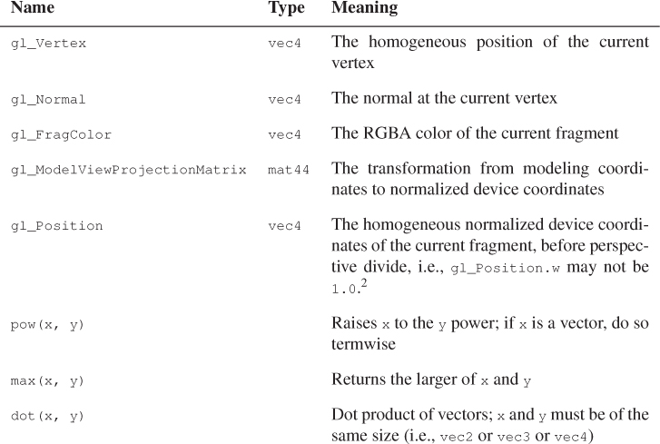
As you can infer from the code, certain variables are predefined in GLSL, as are some useful functions, like normalize and dot. Table 33.1 lists a few of these.
2. In OpenGL these are called “Clip coordinates,” while normalized device coordinates are those after the perspective divide.
Built-in data types include the C-like float and int, and others that help us perform vector operations like vec3 and mat33. GLSL also provides tools for accessing any portion of a vec3 or vec4 through a construction called slicing: If v is a vec3, we can use v.x to access its first entry, and v.yz to access its second and third entries, for instance. Since a vec3 is also used to represent colors (and a vec4 is used to store colors with alpha), we can also write myColor.rga to access the red, green, and alpha portions of a color, for instance. Mixing xyzw-slicing and rgba-slicing is allowed, but seldom makes sense.
As described in Chapter 16, each kind of shader is responsible for establishing values used by later shaders. For instance, a vertex shader like the one used here gets gl_Vertex, the 3D world-space location of the vertex, as input; each time the shader is called, gl_Vertex has a new value, the world-space coordinates for another vertex, in the input. The vertex shader is responsible for assigning a value to gl_Position, which is meant to represent the position of the vertex in camera coordinates, or, expressed alternatively, the position of the vertex after the camera transformation has been applied to move the view frustum to the standard perspective view volume. In the case of our shader, this is accomplished by line 11, which multiplies the vertex coordinates by the appropriate matrix.
A vertex shader may also get other input data, in one of two forms. First, there may be other per-vertex information, like the normal vector, or texture coordinates. Second, there may be information that’s specified per object. In our case, the diffuse reflectivity is one such item (we don’t use it in the vertex shader), and the world-space position of the light is another. That world-space light position is declared uniform vec3 wsLight; the keyword uniform tells GL that the value is set once per object. The declaration of the variable before main indicates that it needs to be linked to the rest of the program. In this case, it’s linked to the host program by a call in ConfigureShaderArgs.
Finally, a vertex shader may set values to be used by other shaders. These values are computed once per vertex; during the rasterization and clipping phase, they’re interpolated to get values at each fragment. The default is perspective interpolation (i.e., barycentric interpolation in camera coordinates), but image-space barycentric interpolation is also an option. The resultant values vary from point to point on the triangle, and so they are declared varying.
Our shader computes one of these, gouraudFactor (line 2), which is the dot product of the unit surface normal and the incoming light direction to the world-space light source.
Having computed this dot product (line 10) and the location of each vertex, we move on to the fragment shader (see Listing 33.4).
Listing 33.4: The fragment shader for the Gouraud shading program.
1 /** Diffuse/ambient surface color */
2 uniform vec3 diffuseColor;
3
4 /** Intensity of the diffuse term. */
5 uniform float diffuse;
6
7 /** Color of the light source */
8 uniform vec3 lightColor;
9
10 /** dot product of surf normal with light */
11 varying float gouraudFactor;
12
13 void main() {
14 gl_FragColor.rgb = diffuse * diffuseColor *
15 (max(gouraudFactor, 0.0) * lightColor);
16 }
Once again, three uniform variables, whose values were established in the host program, get used in the fragment shader: the diffuse reflectivity, the color of the surface, and the color of the light.
We also, in the fragment shader, have access to the gouraudFactor that was computed in the vertex shader. At any fragment, the value for this variable is the result of interpolating the values at the three vertices of the triangle. In the shader, we do a very simple operation: We multiply the diffuse reflectivity by the diffuse color to get a vec3, and multiply the gouraudFactor (if it’s positive) by the light color, giving another vec3. We then take the term-by-term product of these two (using the * operator) and assign it to the gl_FragColor.rgb. If the light is pure red and the surface is pure blue, then the product will be all zeroes. But in general, we are taking the product of the amount of red light and how well the surface reflects red light (and how well it reflects in this direction at all), and similarly for green and blue, to get a color for the fragment.
Every fragment shader is responsible for setting the value of gl_FragColor, which is used by the remainder of the graphics pipeline.
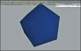
That’s it! This simple host program and two simple shaders implement Gouraud shading. The results are shown in Figure 33.3. In the version of the program available on the book’s website, we’ve added one GUI that allows you to pick a diffuse color and set the reflectivity interactively, and another that allows you to rotate the icosahedron to any position you like, but the essential ideas are unchanged.
33.5. A Phong Shader
In generalizing this to implement the Phong model, there are no real surprises. We have to declare a few more variables in the host program, such as the specular exponent shine, the specular reflection coefficient specular, and the specular color specularColor, and we also include ambient light as ambientLightColor, but we’re confident that you can do this without seeing the code.
Recall that the basic Phong model of Chapter 6 tells us to compute the pixel color using
where kd and ks are the diffuse and specular reflection coefficients, Ia is the ambient light color, Id is the diffuse light color (i.e., the color of our directional light), Od is the diffuse color of the object, ![]() is a unit vector in the direction from the surface point toward the light source, r is the (unit) reflection of the eye vector (the vector from the surface to the eye) through the surface normal, and ns is the specular exponent, or shininess: A small value gives a spread-out highlight; a large value like ns = 500 gives a very concentrated highlight. The formula is only valid if r · n > 0; if it’s negative, the last term gets eliminated.
is a unit vector in the direction from the surface point toward the light source, r is the (unit) reflection of the eye vector (the vector from the surface to the eye) through the surface normal, and ns is the specular exponent, or shininess: A small value gives a spread-out highlight; a large value like ns = 500 gives a very concentrated highlight. The formula is only valid if r · n > 0; if it’s negative, the last term gets eliminated.
In the vertex shader (see Listing 33.5), we compute the normal vector at each vertex, and the ray from the surface point to the eye (at each vertex). We don’t normalize either one yet.
Listing 33.5: The vertex shader for the Phong shading program.
1 /** Camera origin in world space */
2 uniform vec3 wsEyePosition;
3
4 /** Non-unit vector to the eye from the vertex */
5 varying vec3 wsInterpolatedEye;
6
7 /** Surface normal in world space */
8 varying vec3 wsInterpolatedNormal;
9
10 void main(void) {
11 wsInterpolatedNormal = g3d_ObjectToWorldNormalMatrix *
12 gl_Normal;
13 wsInterpolatedEye = wsEyePosition -
14 g3d_ObjectToWorldMatrix * gl_Vertex).xyz;
15
16 gl_Position = gl_ModelViewProjectionMatrix * gl_Vertex;
17 }
In the pixel shader, we take the interpolated values of the normal and eye-ray vectors and use them to evaluate the Phong lighting equation. Even if the normal vector at each vertex is a unit vector, the result of interpolating these will generally not be a unit vector. That’s why we didn’t bother normalizing them in the vertex shader: We’ll need to do a normalization at each pixel anyhow. After normalizing these, we compute the reflected eye vector r, and use it in the Phong equation to evaluate the pixel color. Note the use of max (line 32) to eliminate the case where the reflected eye vector is not in the same half-space as the ray to the light source. (See Listing 33.6.)
Listing 33.6: The fragment shader for the Phong shading program.
1 /** Diffuse/ambient surface color */
2 uniform vec3 diffuseColor;
3 /** Specular surface color, for glossy and mirror refl’n. */
4 uniform vec3 specularColor;
5 /** Intensity of the diffuse term. */
6 uniform float diffuse;
7 /** Intensity of the specular term. */
8 uniform float specular;
9 /** Phong exponent; 100 = sharp highlight, 1 = broad highlight */
10 uniform float shine;
11 /** Unit world space dir’n to (infinite, directional) light */
12 uniform vec3 wsLight;
13 /** Color of the light source */
14 uniform vec3 lightColor;
15 /** Color of ambient light */
16 uniform vec3 ambientLightColor;
17 varying vec3 wsInterpolatedNormal;
18 varying vec3 wsInterpolatedEye;
19
20 void main() {
21 // Unit normal in world space
22 vec3 wsNormal = normalize(wsInterpolatedNormal);
23
24 // Unit vector from the pixel to the eye in world space
25 vec3 wsEye = normalize(wsInterpolatedEye);
26
27 // Unit vector giving the dir’n of perfect reflection into eye
28 vec3 wsReflect = 2.0 * dot(wsEye, wsNormal) * wsNormal - wsEye;
29
30 gl_FragColor.rgb = diffuse* diffuseColor*
31 (ambientLightColor +
32 (max(dot(wsNormal, wsLight), 0.0) * lightColor)) +
33 specular * specularColor *
34 pow(max(dot(wsReflect, wsLight), 0.0), shine) * lightColor;
35 }
33.6. Environment Mapping
To implement environment mapping (see Section 20.2.1), we can use the same vertex shader as before to compute the interpolated eye vector and normal vector. Rather than computing the diffuse or specular lighting, we can use the reflected vector to index into an environment map, which is specified by a set of six texture maps (see Figure 33.4). The host program must load these six maps and make them available to the shader; to do so, we declare a new member variable in the App class and then, during initialization of the application, invoke
environmentMap = Texture::fromFile("uffizi*,png", ...)
to load the cube map with one of G3D’s built-in procedures. Within the configureShaderArgs procedure, we must add
myShader->args.set("environmentMap", environmentMap);
to link the host-program variable to a shader variable.
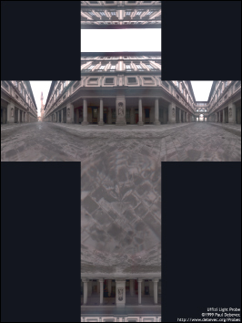
Figure 33.4: An environment map of the Uffizi, specified by six texture maps, one each for the top, bottom, and four vertical sides of a cube, displayed here in a cross-layout. (Courtesy of Paul Debevec. Photographs used with permission. ©2012 University of Southern California, Institute for Creative Technologies.)
The fragment shader (see Listing 33.7) is very simple: A fragment is colored by using its normal vector as an index into the cube map, via a GLSL built-in. The color that’s returned is multiplied by the specular color for the model (which we set to a very pale gold) so that the reflections take on the color of the surface, simulating a metallic surface, rather than retaining their own color, as would occur with a plastic surface.
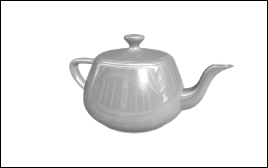
The result (see Figure 33.5) shows a shiny teapot reflecting the plaza of the Uffizi gallery using the environment map we showed earlier.
Anytime a shader uses a texture, the texture is automatically MIP-mapped for you by GL (unless you explicitly request that it not be). The semantics of GL are such that the derivative of any quantity with respect to pixel coordinates can be computed at any point where the quantity is defined. So at each point where the teapot appears in the image, the rates of change of the coordinates of the normal vector with respect to the pixel coordinates are computed and used to select a MIP-mapping level that’s appropriate.
Listing 33.7: The fragment shader for the Phong shading program.
1 /** Unit world space direction to the (infinite, directional)
2 light source */
3 uniform vec3 wsLight;
4
5 /** Environment cube map used for reflections */
6 uniform samplerCube environmentMap;
7
8 /** Color for specular reflections */
9 uniform vec3 specularColor;
10
11 varying vec3 wsInterpolatedNormal;
12 varying vec3 wsInterpolatedEye;
13
14 void main() {
15 // Unit normal in world space
16 vec3 wsNormal = normalize(wsInterpolatedNormal);
17
18 // Unit vector from the pixel to the eye in world space
19 vec3 wsEye = normalize(wsInterpolatedEye);
20
21 // Unit vector giving direction of reflection into the eye
22 vec3 wsReflect = 2.0 * dot(wsEye, wsNormal)
23 * wsNormal - wsEye;
24
25 gl_FragColor.rgb =
26 specularColor * textureCube(environmentMap,
27 wsReflect).rgb;
28 }
33.7. Two Versions of Toon Shading
We now turn to a rather different style, the toon shading of Chapter 34. In toon shading, we compute the dot product of the normal and the light direction (as we would for any Lambertian surface), but then choose a color value by thresholding the result so that the resultant picture is drawn with just two or three colors, much as a cartoon might be. There are, of course, many possible variations: We could do thresholded shading using the Phong model, or any other; we could use two or five thresholds; we could have varying light intensity rather than the simple “single bright light” model we’re using here.
The first (and not very wise) approach we’ll take is to compute the intensity (the dot product of the normal and light vectors) at each vertex in the vertex shader (Listing 33.8), and let GL interpolate this value across each triangle and then threshold the resulting intensities (Listing 33.9).
Listing 33.8: The vertex shader for the first toon-shading program.
1 /* Camera origin in world space */
2 uniform vec3 wsEyePosition;
3 /* Non-unit vector to eye from vertex */
4 varying vec3 wsInterpolatedEye;
5 /* Non-unit surface normal in world space */
6 varying vec3 wsInterpolatedNormal;
7 /* Unit world space dir’n to directional light source */
8 uniform vec3 wsLight;
9 /* the "intensity" that we’ll threshold */
10 varying float intensity;
11
12 void main(void) {
13 wsInterpolatedNormal =
14 normalize(g3d_ObjectToWorldNormalMatrix * gl_Normal);
15 wsInterpolatedEye =
16 wsEyePosition - (g3d_ObjectToWorldMatrix * gl_Vertex).xyz;
17
18 gl_Position = gl_ModelViewProjectionMatrix * gl_Vertex;
19 intensity = dot(wsInterpolatedNormal, wsLight);
20 }
Listing 33.9: The pixel shader for the first toon-shading program.
1 ... same declarations ...
2 void main() {
3 if (intensity > 0.95)
4 gl_FragColor.rgb = diffuseColor;
5 else if (intensity > 0.5)
6 gl_FragColor.rgb = diffuseColor * 0.6;
7 else if (intensity > 0.25)
8 gl_FragColor.rgb = diffuseColor * 0.4;
9 else
10 gl_FragColor.rgb = diffuseColor * 0.2;
11 }
The results, shown in Figure 33.6, are unsatisfactory: When the intensity is linearly interpolated across a triangle and then thresholded, the result is a straight-line boundary between the two color regions. When this is done for every polygon, the result is that each color region has a visibly polygonal boundary.

We can improve this substantially by using the interpolated surface normal and interpolated light vector in the fragment shader to compute an intensity value that varies smoothly across the polygon, and which, when thresholded, produces a smooth boundary between color regions. In our case, with a directional light, only the interpolation of the surface normal has an effect, but the program would also work for more general lights.
This program gives yet another instance of the principle that not every pair of operations commutes, and swapping the order for simplicity or efficiency only works acceptably in some cases. Explain which two operations are not commuting in this example.
The revised program can use exactly the same vertex shader, except that we no longer need to declare or compute intensity. The revised fragment shader is shown in Listing 33.10, and the results are shown in Figure 33.7.

Figure 33.7: Toon shading using a fragment shader. Notice the smooth boundary between the shades of red.
Notice that in the fragment shader, we took the normal vector that was computed at each vertex, and then interpolated to the current fragment, and normalized it.
Listing 33.10: The fragment shader for the improved toon-shading program.
1 uniform vec3 diffuseColor; /* Surface color */
2 uniform vec3 wsLight; /* Unit world sp. dir’n to light */
3 varying vec3 wsInterpolatedNormal; /* Surface normal. */
4
5 void main() {
6 float intensity = dot(normalize(wsInterpolatedNormal),wsLight);
7 if (intensity > 0.95)
8 gl_FragColor.rgb = diffuseColor;
9 else if (intensity > 0.4)
10 gl_FragColor.rgb = diffuseColor * 0.6;
11 else
12 gl_FragColor.rgb = diffuseColor * 0.2;
13 }
Suppose we had omitted the normalization in the fragment shader in Listing 33.10. How would the resultant image have differed? How would it have differed from our first-draft toon shader? If you don’t know, implement both and compare.
33.8. Basic XToon Shading
Finally, we provide an implementation of a tiny portion of XToon shading: a shader where a 2D texture map (see Figure 33.8) is used to govern appearance, but in a somewhat unusual way. We index into the vertical coordinate using distance from the eye so that more-distant points are bluer, resulting in a weak approximation of atmospheric perspective, which is based on the observation that in outdoor scenes, more-distant objects (e.g., mountains) tend to look bluer, and hence we can provide a distance cue by mimicking this. We index into the horizontal coordinate using the dot product of the view vector with the normal vector. Whenever this dot product is zero (i.e., on a contour), we index into mid texture (i.e., the black area), resulting in black contour lines being drawn. In our texture, we’ve made the black line larger at the bottom than the top, resulting in wider contours at distant points than at nearby ones; endless other stylistic variations are possible.
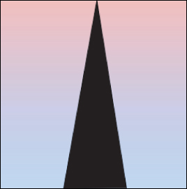
Figure 33.8: The 2D texture map for XToon shading. We use distance as an index into the vertical direction, and v·n as the horizontal index.
The shader code is once again very simple. In the vertex shader, we compute the distance to the eye at each vertex; see Listing 33.11.
The results are shown in Figure 33.9. The teapot’s contours are drawn with gray-to-black lines, thicker in the distance; the handle of the teapot is slightly bluer than the spout.

Listing 33.11: The vertex and fragment shaders for the XToon shading program.
1 ... Vertex Shader ...
2 uniform vec3 wsEyePosition;
3 varying vec3 wsInterpolatedEye;
4 varying vec3 wsInterpolatedNormal;
5
6 varying float dist;
7
8 void main(void) {
9 wsInterpolatedNormal =
10 normalize(g3d_ObjectToWorldNormalMatrix * gl_Normal);
11 wsInterpolatedEye = wsEyePosition -
12 (g3d_ObjectToWorldMatrix * gl_Vertex).xyz;
13 gl_Position = gl_ModelViewProjectionMatrix * gl_Vertex;
14 dist = sqrt(dot(wsInterpolatedEye, wsInterpolatedEye));
15 }
16
17 ... Fragment Shader ...
18 varying vec3 wsInterpolatedNormal;
19 varying vec3 wsInterpolatedEye;
20 varying float dist;
21
22 void main() {
23 vec3 wsNormal = normalize(wsInterpolatedNormal);
24 vec3 wsEye = normalize(wsInterpolatedEye);
25 vec2 selector; // index into texture map
26 selector.x = (1.0 + dot(wsNormal, wsEye))/2.0; // in [0 1]
27 selector.y = dist/2; // scaled to account for size of teapot
28 gl_FragColor.rgb = texture2D(xtoonMap, selector).rgb;
29 }
33.9. Discussion and Further Reading
As we discussed in this chapter and what we should include as examples, one of us said, “I worry that what you guys call shaders are what I call graphics!” His point was a good one: Phong shading involves the same computation whether you do it on the CPU or on the GPU. The choice of where to implement a particular aspect of your graphics program is a matter of engineering: What works best for your particular situation? Since GPUs are becoming increasingly parallelized, and branching tends to damage throughput, a rough guideline is that branch-intensive code should run on the CPU and straight-line code on the GPU. But with tricks like hiding an if statement by adding arithmetic, as in using
x = (u == 1) * y + (u != 1) * z
as a replacement for
if (u == 1) then x = y else x = z
you can see that there’s no hard-and-fast rule. The factors that may weigh in the decision are software development costs, bandwidth to/from the GPU, and the amount of data that must be passed between various shaders on the GPU.
New books of shader tricks are being published all the time. Many of the tricks described in these books are ways to get around the limitations of current GPU hardware or software architecture, and they tend to be out of date almost as soon as the books are published. Others have longer-term value, demonstrating how the work in some algorithm is best partitioned among various shader stages.
33.10. Exercises
For all these exercises, you’ll need a GL wrapper like G3D, or else a shader development tool like RenderMonkey [AMD12], to experiment with.
Exercise 33.1: Write a vertex shader that alters the x-coordinate of every point on an object as a sinusoidal function of its y-coordinate.
Exercise 33.2: Write a vertex shader that alters the x-coordinate of each surface point as a sinusoidal function of y and time (which you’ll need to pass to the shader from the host program, which will get the time from the system clock). You’ll write something like
gl_Position.x += sin(k1 * gl_Position.y - k2 * t);
which will produce waves of wavelength ![]() , moving with velocity
, moving with velocity ![]() .
.
Exercise 33.3: Write a vertex shader that draws each triangle in a different (flat) color, specified by the host program. This can be very useful for debugging.