
Chapter 36. Visibility Determination
36.1. Introduction
Determining the visible parts of surfaces is a fundamental graphics problem. It arises naturally in rendering because rendering objects that are unseen is both inefficient and incorrect. This problem is called either visible surface determination or hidden surface removal, depending on the direction from which it is approached.
The two distinct goals for visibility are algorithm correctness and efficiency. A visibility algorithm responsible for the correctness of rendering must exactly determine whether an unobstructed line of sight exists between two points, or equivalently, the set of all points to which one point has an unobstructed line of sight. The most intuitive application is primary visibility: Solve visibility exactly for the camera. Doing so will only allow the parts of the scene that are actually visible to color the image so that the correct result is produced. Ray casting and the depth buffer are by far the most popular methods for ensuring correct visibility today.
A conservative visibility algorithm is designed for efficiency. It will distinguish the parts of the scene that are likely visible from those that are definitely not visible, with respect to a point. Conservatively eliminating the nonvisible parts reduces the number of exact visibility tests required but does not guarantee correctness by itself. When a conservative result can be obtained much more quickly than an exact one, this speeds rendering if the conservative algorithm is used to prune the set that will be considered for exact visibility. For example, it is more efficient to identify that the sphere bounding a triangle mesh is behind the camera, and therefore invisible to the camera, than it is to test each triangle in the mesh individually.
Backface culling and frustum culling are two simple and effective methods for conservative visibility testing; occlusion culling is a more complex refinement of frustum culling that takes occlusion between objects in the scene into account. Sophisticated spatial data structures have been developed to decrease the cost of conservative visibility testing. Some of these, such as the Binary Space Partition (BSP) tree and the hierarchical depth buffer, simultaneously address both efficient and exact visibility by incorporating conservative tests into their iteration mechanism. But often a good strategy is to combine a conservative visibility strategy for efficiency with a precise one for correctness.
![]() The Culling Principle
The Culling Principle
It is often efficient to approach a problem with one or more fast and conservative solutions that narrow the space by culling obviously incorrect values, and a slow but exact solution that then needs only to consider the fewer remaining possibilities.
Primary visibility tells us which surfaces emit or scatter light toward a camera. They are the “last bounce” locations under light transport and are the only surfaces that directly affect the image. However, keep in mind that a global illumination renderer cannot completely eliminate the points that are invisible to the camera. This is because even though a surface may not directly scatter light toward the camera, it may still affect the image. Figure 36.1 shows an example in which removing a surface that is invisible to the camera changes the image, since that surface casts light onto surfaces that are visible to the camera. Another example is a shadow caster that is not visible, but casts a shadow on points that are visible to the camera. Removing the shadow caster from the entire rendering process would make the shadow disappear. So, primary visibility is an important subproblem that can be tackled with visibility determination algorithms, but it is not the only place where we will need to apply those algorithms.
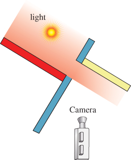
Figure 36.1: The yellow wall is illuminated only by light reflected from the hidden red polygon. Removing it will cause the yellow wall to be illuminated only by light from the blue surface.
The importance of indirect influence on the image due to points not visible to the camera is why we define exact visibility as a property that we can test for between any pair of points, not just between the camera and a scene point. A rendering algorithm incorporating global illumination must consider the visibility of each segment of a transport path from the source through the scene to the camera. Often the same algorithms and data structures can be applied to primary and indirect visibility. For example, the shadow map from Chapter 15 is equivalent to a depth buffer for a virtual camera placed at a light source.
There are of course nonrendering applications of algorithms originally introduced for visibility determination. Collision detection for the simulation of fast-moving particles like bullets and raindrops is often performed by tracing rays as if they were photons. Common modeling intersection operations such as cutting one shape out of another are closely related to classic visibility algorithms for subdividing surfaces along occlusion lines.
The motivating examples throughout this chapter emphasize primary visibility. That’s because it is perhaps the most intuitive to consider, and because the camera’s center of projection is often the single point that appears in the most visibility tests. For each example, consider how the same principles apply to general visibility tests. As you read about each data structure, think in particular about how many visibility tests at a point are required to amortize the overhead of building that data structure.
In this chapter, we first present a modern view of visibility following the light transport literature. We formally frame the visibility problem as an intersection query for a ray (“What does this ray hit first?”) and as a visibility function on pairs of points (“Is Q visible from P?”). We then describe algorithms that can amortize that computation when it is performed conservatively over whole primitives for efficient culling. This isn’t the historical order of development. In fact, the topic developed in the opposite order.
Historically, the first notion of visibility was the question “Is any part of this triangle visible?” That grew more precise with “How much of this triangle is visible?” which was a critical question when all rendering involved drawing edges on a monochrome vector scope or rasterizing triangles on early displays and slow processors. With the rise of ray tracing and general light transport algorithms, a new visibility question was framed on points. That then gave a formal definition for the per-primitive questions, which expanded under notions of partial coverage to the framework encountered today. Of course, classic graphics work on primitives was performed with an understanding of the mathematics of intersection and precise visibility. The modern notion is just a redirection of the derivation: working up from points and rays with the rendering equation in mind, rather than down from surfaces under an ad hoc illumination and shading model.
36.1.1. The Visibility Function
Visible surface determination algorithms are grounded in a precise definition of visibility. We present this formally here in terms of geometry as the basis for the high-level algorithms. While it is essential for defining and understanding the algorithms, this direct form is rarely employed.
A performance reason that we can’t directly apply the definition of visibility is that with large collections of surfaces in a scene, exhaustive visibility testing would be inefficient. So we’ll quickly look for ways to amortize the cost across multiple surfaces or multiple point pairs.
A correctness concern with direct visibility is that under digital representations, the geometric tests involved in single tests are also very brittle. In general, it is impossible to represent most of the points on a line in any limited-precision format, so the answer to “Does this point occlude that line of sight?” must necessarily almost always be “no” on a digital computer. We can escape the numerical precision problem by working with spatial intervals—for example, line segments, polygons, and other curves—for which occlusion of a line of sight is actually representable, but we must always implicitly keep in mind the precision limitation at the boundaries of those intervals. Thus, the question of whether a ray passes through a triangle if it only intersects the edge is moot. In general, we can’t even represent that intersection location in practice, so our classification is irrelevant. So, beware that everything in this chapter is only valid in practice when we are considering potential intersections that are “far away” from surface boundaries with respect to available precision, and the best that we can hope for near boundaries is a result that is spatially coherent rather than arbitrarily changing within the imprecise region.
Given points P and Q in the scene, let visibility function V(P, Q) = 1 if there is no intersection between the scene and the open-ended line segment between P and Q, and V(P, Q) = 0 otherwise. This is depicted in Figure 36.2. Sometimes it is convenient to work with the occlusion function H(P, Q) = 1 – V(P, Q). The visibility function is necessarily symmetric, so V(P, Q) = V(Q, P).
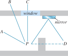
Figure 36.2: V(P, A) = 1 because there is no occluder. V(P, B) = 0 because a wall is in the way. V(P, C) = 0 because, even though P can see C through the window, the window is an occluder as far as mathematical “visibility” is concerned. Likewise, V(P, D) = 0, even though P sees a reflection of D in the mirror.
Note that the “visibility” in “visibility function” refers strictly to geometric line-of-sight visibility. If P and Q are separated by a pane of glass, V(P, Q) is zero because a nonempty part of the scene (the glass pane) is intersected by the line segment between P and Q. Likewise, if an observer at Q has no direct line of sight to P, but can see P through a mirror or see its shadow, we still say that there is no direct visibility: V(P, Q) = 0.
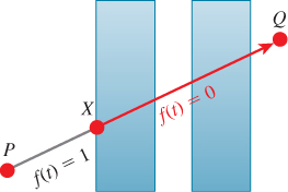
Let X be the first scene point encountered along a ray with origin P in direction ![]() . Point X partitions the ray into two visibility ranges. To see this, define f to be visibility as a function of distance from Q, that is, let
. Point X partitions the ray into two visibility ranges. To see this, define f to be visibility as a function of distance from Q, that is, let ![]() . Between X and P, 0 ≤ t ≤ |X ≈ P|, there is visibility, so f(t) = 1 as shown in Figure 36.3. Beyond X, t > ||X – P||. For that domain there is no visibility because X is an occluder, so f(t) = 0.
. Between X and P, 0 ≤ t ≤ |X ≈ P|, there is visibility, so f(t) = 1 as shown in Figure 36.3. Beyond X, t > ||X – P||. For that domain there is no visibility because X is an occluder, so f(t) = 0.
Evaluating the visibility function is mathematically equivalent to finding that first occluding point X, given a starting point P and ray direction ![]() . The first occluding point along a ray is the solution to a ray intersection query. Chapter 37 presents data structures for efficiently solving ray intersection queries. It is not surprising that a common way to evaluate V(P, Q) is to solve for X. If X exists and lies on the line segment PQ, then V(P, Q) = 0; otherwise, V(P, Q) = 1.
. The first occluding point along a ray is the solution to a ray intersection query. Chapter 37 presents data structures for efficiently solving ray intersection queries. It is not surprising that a common way to evaluate V(P, Q) is to solve for X. If X exists and lies on the line segment PQ, then V(P, Q) = 0; otherwise, V(P, Q) = 1.
Some rendering algorithms explicitly evaluate the visibility function between pairs of points by testing for any intersection between a line segment and the surfaces in a scene. Examples include direct illumination shadow tests in a ray tracer and transport path testing in bidirectional path tracing [LW93, VG94], and Metropolis light transport [VG97].
Others solve for the first intersection along a ray instead, thus implicitly evaluating visibility by only generating the visible set of points. Examples include primary and recursive rays in a ray tracer and deferred-shading rasterizers. These are all algorithms with explicit visibility determination. They resolve visibility before computing transport (often called “shading” in the real-time rendering community) between points, thus avoiding the cost of scattering computations for points with no net transport. Simpler renderers compute transport first and rely on ordering to implicitly resolve visibility. For example, a naive ray tracer might shade every intersection encountered along a ray, but only retain the radiance computed at the one closest to the ray origin. This is equivalent to an (also naive) rasterization renderer that does not make a depth prepass. Obviously it is preferable to evaluate visibility before shading in cases where the cost of shading is relatively high, but whether to evaluate that visibility explicitly or implicitly greatly depends on the particular machine architecture and scene data structure. For example, rasterization renderers prefer a depth prepass today because the memory to store a depth buffer is now relatively inexpensive. Were the cost of a full-screen buffer very expensive compared to the cost of computation (as it once was, and might again become if resolution or manufacturing changes significantly), then a visibility prepass might be the naive choice and some kind of spatial data structure again dominate rasterization rendering.
Observe that following conventions from the literature, we defined the visibility function on the open line segment that does not include its endpoints. This means that if the ray from P to Q first meets scene geometry at a point X different from P, then V(P, X) = 1. This is a convenient definition given that the function is typically applied to points on surfaces. Were we to consider the closed line segment, then there would never be any visibility between the surfaces of a scene—they would all occlude themselves. We would have to consider points slightly offset from the surfaces in light transport equations.
In practice, the distinction between open and closed visibility only simplifies the notation of transport equations, not implementations in programs. That is because rounding operations implicitly occur after every operation when working with finite-precision arithmetic, introducing small-magnitude errors (see Figure 36.5). So we must explicitly phrase all applications of the visibility function and all intersection queries with some small offset. This is often called ray bumping because it “bumps” the origin of the visibility test ray a small distance from the starting surface. Note that the bumping must happen on the other end as well. For example, to evaluate V(Q, P), attempt to find a scene point X = Q+S(Q – P)t for < t < |P–Q|–![]() . If and only if there is no scene point satisfying that constraint, then V(Q, P) = 1. Failing to choose a suitably large
. If and only if there is no scene point satisfying that constraint, then V(Q, P) = 1. Failing to choose a suitably large ![]() value can produce artifacts such as shadow acne (i.e., self-shadowing), speckled highlights and reflections, and darkening of the indirect components of illumination shown in Figure 36.4. The noisy nature of these artifacts arises from the sensitivity of the comparison operations to the small-magnitude representation error in the floating-point values.
value can produce artifacts such as shadow acne (i.e., self-shadowing), speckled highlights and reflections, and darkening of the indirect components of illumination shown in Figure 36.4. The noisy nature of these artifacts arises from the sensitivity of the comparison operations to the small-magnitude representation error in the floating-point values.
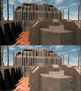
Figure 36.4: (Top) Self-occlusion from insufficient numerical precision or offset values causes the artifacts of shadow acne and speckling in indirect illumination terms such as mirror reflections. (Bottom) The same scene with the shadow acne removed.
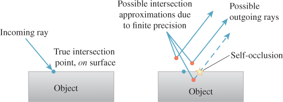
Figure 36.5: Finite precision leads to self-occlusions. “Bumping” the outgoing ray biases the representation error in a direction less likely to produce artifacts by favoring the points above the surface as the ray origin.
36.1.2. Primary Visibility
Primary visibility (a.k.a. eye ray visibility, camera visibility) is visibility between a point on the aperture of a camera and a point in the scene. To render an image, one visibility test must be performed per light ray sample on the image plane. In the simplest case, there is one sample at the center of each pixel. Computing multiple samples at each pixel often improves image quality. See Section 36.9 for a discussion of visibility in the presence of multiple samples per pixel.
A pinhole camera has a zero-area aperture, so for each sample point on the image plane there is only one ray along which light can travel. That is the primary ray for that point on the image plane. Consider three points on the primary ray: sample point Q on the imager, the aperture A, and a point P in the scene. Since there are no occluding objects inside the camera, V(Q, P) = V(A, P).
Since the visibility function evaluations or intersection queries at all samples share a common endpoint of the pinhole aperture, there are opportunities to amortize operations across the image. Ray packet tracing and rasterization are two algorithms that exploit this technique. For more details, see Chapter 15, which develops the amortized aspect of rasterization and presents the equivalence of intersection queries under rasterization and ray tracing.
36.1.3. (Binary) Coverage
Coverage is the special case of visibility for points on the image plane. For a scene composed of a single geometric primitive, the coverage of a primary ray is a binary value that is 1 if the ray intersects the primitive between the image plane and infinity, and 0 otherwise. This is equivalent to the visibility function applied to the primary ray origin and a point infinitely far away along the primary ray.
For a scene containing multiple primitives, primitives may occlude each other in the camera’s view. The depth complexity of a ray is the number of times it intersects the scene. At any given intersection point P, the quantitative invisibility [App67] is the number of other primitive intersections that lie between the ray origin and P. Figure 36.6 shows examples of each of these concepts.
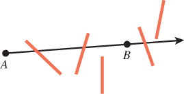
Figure 36.6: The quantitative invisibility of two points is the number of surface intersections on the segment between them. The quantitative invisibility of B with respect to A is 2 in this figure. The depth complexity of a ray is the total number of surface intersections along the ray. The ray from A through B has depth complexity 3 in this figure.
For some applications, backfaces—surfaces where the dot product of the geometric normal and the ray direction is positive—are ignored when computing depth complexity and quantitative invisibility. The case where the intersection of the ray and a surface is a segment (e.g., Figure 36.7) instead of a finite number of points is tricky. We’ve already discussed that the existence of such an intersection is already suspect due to limited precision, and in fact for it to occur at all with nonzero probability requires us to have explicitly placed geometry in just the right configuration to make such an unlikely intersection representable. Of course, humans are very good at constructing exactly those cases, for example, by placing edges at perfectly representable integer coordinates and aligning surfaces with axes in ways that could never occur in data measured from the real world. We note that for a closed polygonal model, it is common to ignore these line-segment intersections, but the definition of depth complexity and quantitative invisibility for this case varies throughout the literature.

In the case of multiple primitive intersections, we say that the coverage is 1 at the first intersection and 0 at all later ones to match the visibility function definition.
At the end of this chapter, in Section 36.9, we extend binary coverage to partial coverage by considering multiple light paths per pixel.
36.1.4. Current Practice and Motivation
Most rendering today is on triangles. The triangles may be explicitly created, or they may be automatically generated from other shapes. Some common modeling primitives that are reducible to triangles are subdivision surfaces, implicit surfaces, point clouds, lines, font glyphs, quadrilaterals, and height field models.
Ray-tracing renderers solve exact visibility determination by ray casting (Section 36.2): intersecting the model with a ray to produce a sample. Data structures optimized for ray-triangle intersection queries are therefore important for efficient evaluation of the visibility function. Chapter 37 describes several of these data structures. Backface culling (Section 36.6) is implicitly part of ray casting.
Hardware rasterization renderers today tend to use frustum culling (Section 36.5), frustum clipping (Section 36.5), backface culling (Section 36.6), and a depth buffer (Section 36.3) for per-sample visible surface determination. Those methods provide correctness, but they require time linear in the number of primitives. So relying on them exclusively would not scale to large scenes. For efficiency it is therefore necessary to supplement those with conservative methods for determining occlusion and hierarchical methods for eliminating geometry outside the view frustum in sublinear time.
A handful of applications rely on the painter’s algorithm (Section 36.4.1) of simply drawing everything in the scene in back-to-front order and letting the ordering resolve visibility. This is neither exact nor conservative1, but it has the benefit of extreme simplicity. It is used almost exclusively for 2D graphical user interface rendering to handle overlapping windows. The primary 3D application of the painter’s algorithm today is for rasterization of translucent surfaces, although recent trends favor more accurate per-sample stochastic and lossy-volumetric alternatives [ESSL10, LV00, Car84, SML11, JB10, MB07].
1. . . . nor how artists actually paint—for example, sometimes the sky is painted after foreground objects—but the name is now both a technical term and appropriately evocative.
Many applications combine multiple visibility determination algorithms. For example, a hybrid renderer might rasterize primary and shadow rays but perform ray casting for visibility determination on other global illumination paths. A realtime hardware rasterization renderer might augment its depth buffer with hierarchical occlusion culling or precomputed conservative visibility. Many games rely on those techniques, but they include a ray-casting algorithm for visibility determination used to determine line of sight for character AI logic and physical simulation.
36.2. Ray Casting
Ray casting is a direct process for answering an intersection query. As previously shown, it also computes the visibility function: V(P, Q) = 1, if P is the result of the intersection query on the ray with origin Q and direction (P – Q)/|P – Q|; and V(P, Q) = 0 otherwise. Chapter 15 introduced an algorithm for casting rays in scenes described by arrays of triangles, and showed that the same algorithm can be applied to primary and indirect (in that case, shadow) visibility.
The time cost of casting a ray against n triangles in an array is O(n) operations. If V(P, Q) = 1, then the algorithm must actually test every ray-triangle pair. If V(P, Q) = 0, then the algorithm can terminate early when it encounters any intersection with the open segment PQ. In practice this means that computing the visibility function by ray casting may be faster than solving the intersection query; hence, resolving one shadow ray may be faster than finding the surface to shade for one ray from the camera. For a dense scene with high depth complexity, the performance ratio between them may be significant.
Terminating on any intersection still only makes ray casting against an array of surfaces faster by a constant, so it still requires O(n) operations for n surfaces. Linear performance is impractical for large and complex scenes, especially given that such scenes are exactly those in which almost all surfaces are not visible from a given point. Thus, there are few cases in which one would actually cast rays against an array of surfaces, and for almost all applications some other data structure is used to achieve sublinear scaling.
Chapter 37 describes many spatial data structures for accelerating ray intersection queries. These can substantially reduce the time cost of visibility determination compared to the linear cost under an array representation. However, building such a structure may only be worthwhile if there will be many visibility tests over which to amortize the build time. Constants vary with algorithms and architectures, but for more than one hundred triangles or other primitives and a few thousand visibility tests, building some kind of spatial data structure will usually provide a net performance gain.
We now give an example of how a ray-primitive intersection query operates within the binary space partition tree data structure. The issues encountered in this example apply to most other spatial data structures, including bounding volume hierarchies and grids.
36.2.1. BSP Ray-Primitive Intersection
The binary space partition tree (BSP tree) [SBGS69, FKN80] is a data structure for arranging geometric primitives based on their locations and extents. Chapter 37 describes in detail how to build and maintain such a structure, and some alternative data structures. The BSP tree supports finding the first intersection between a ray and a primitive. The algorithm for doing this often has only logarithmic running time in the number of primitives. We say “often” because there are many pathological tree structures and scene distributions that can make the intersection time linear, but these are easily avoidable for many scenes. This logarithmic scaling makes ray casting practical for large scenes.
The BSP tree can also be used to compute the visibility function. The algorithm for this is nearly identical to the first-intersection query. It simply terminates with a return value of false when any intersection is detected, and returns true otherwise.
There are a few variations on the BSP structure. For the following example, we consider a simple one to focus on the algorithm. In our simple tree, every internal node represents a splitting plane (which is not part of the scene geometry) and every leaf node represents a geometric primitive in the scene. A plane divides space into two half-spaces. Let the positive half-space contain all points in the plane and on the side to which the normal points. Let the negative half-space contain all points in the plane and on the side opposite to which the normal points. Figure 36.8 shows one such plane (for a 2D scene, so the “plane” is a line). Both the positive and negative half-spaces will be subdivided by additional planes when creating a full tree, until each sphere primitive is separated from the others by at least one plane.
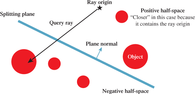
Figure 36.8: The splitting plane for a single internal BSP node divides this scene composed of five spheres into two half-spaces.
The internal nodes in the BSP tree have at most two children, which we label positive and negative. The construction algorithm for the tree ensures that the positive subtree contains only primitives that are in the positive half-space of the plane (or on the plane itself) and that the negative subtree contains only those in the negative half-space of the plane. If a primitive from the scene crosses a splitting plane, then the construction algorithm divides it into two primitives, split at that plane.
Listing 36.1 gives the algorithm to evaluate the visibility function in this simple BSP tree. The recursive intersects function performs the work. Point Q is visible to point P if no intersection exists between the line segment PQ and the geometry in the subtree with node at its root. When node is a leaf, it contains one geometric primitive, so intersects tests whether the line-primitive intersection is empty. Chapter 7 describes intersection algorithms that implement this test for different types of geometric primitives, and Chapter 15 contains C++ code for ray-triangle intersection.
Figure 36.9 visualizes the algorithm’s iteration through a 2D tree for a scene consisting of disks.
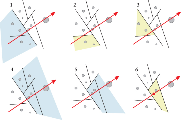
Figure 36.9: Tracing a ray through a scene containing disks stored in a 2D BSP tree. Highlighted portions of space correspond to the node at which the algorithm is operating in each step. Iteration proceeds depth-first, preferring to descend into the geometrically closer of the two children at each node.
If node is an internal node, then it contains a splitting plane that creates two half-spaces. We categorize the child nodes corresponding to these as being closer and farther with respect to P. Figure 36.8 shows an example classification at an internal node. With an eye toward reusing this algorithm’s structure for the related problem of finding the first intersection, we choose to visit the closer node first. That is because if there is any intersection between segment PQ and the scene in closer, it must be closer to P than every intersection in farther [SBGS69].
If PQ lies entirely in one half-space, the result of the intersection test for the current node reduces to the result of the test on that half-space. Otherwise, there is an intersection if one is found in either half-space, so the algorithm recursively visits both.
Listing 36.1: Pseudocode for visibility testing in a BSP tree.
1 function V(P, Q):
2 return not intersects(P, Q, root)
3
4 function intersects(P, Q, node):
5 if node is a leaf:
6 return (PQ intersects the primitive at the node)
7
8 closer = node.positiveChild
9 farther = node.negativeChild
10
11 if P is in the negative half-space of node:
12 // The negative side of the plane is closer to P
13 swap closer, farther
14
15 if intersects(P, Q, closer):
16 // Terminate early because an intersection was found
17 return true
18
19 if P and Q are in the same half-space of node:
20 // Segment PQ does not extend into the farther side
21 return false
22
23 // After searching the closer side, recursively search
24 // for an intersection on the farther side
25 return intersects(P, Q, farther)
The visibility testing code assumes that there’s a closer and a farther half-space. What will this code do when the splitting plane contains the camera point P? Will it still perform correctly? If not, what modifications are needed?
In the worst case the routine must visit every node of the tree. In practice this rarely occurs. Typically, PQ is small with respect to the size of the scene and the planes carve space into convex regions that do not all lie along the same line. So we expect a relatively tight depth-first search with runtime proportional to the height of the tree.
There are many ways to improve the performance of this algorithm by a constant factor. These include clever algorithms for constructing the tree and extending the binary tree to higher branching factors. For sparse scenes, alternative spatial partitions can be advantageous. The convex spaces created by the splitting planes often have a lot of empty space compared to the volumes bounded by the geometric primitives within them in a BSP tree. A regular grid or bounding volume hierarchy may increase the primitive density within leaf nodes, thus reducing the number of primitive intersections performed.
Where BSP tree iteration is limited by memory bandwidth, substantial savings can be gained by using techniques for compressing the plane and node pointer representation [SSW+06].
36.2.2. Parallel Evaluation of Ray Tests
The previous analysis considered serial processing on a single scalar core. Parallel execution architectures change the analysis. Tree search is notoriously hard to execute concurrently for a single query. Near the root of a tree there isn’t enough work to distribute over multiple execution units. Deeper in the tree there is plenty of work, but because the lengths of paths may vary, the work of load balancing across multiple units may dominate the actual search itself. Furthermore, if the computational units share a single global memory, then the bandwidth constraints of that memory may still limit net performance. In that case, adding more computational units can reduce net performance because they will overwhelm the memory and reduce the coherence of memory access, eliminating any global cache efficiency.
There are opportunities for scaling nearly linearly in the number of computational units when performing multiple visibility queries simultaneously, if they have sufficient main memory bandwidth or independent on-processor caches. In this case, all threads can search the tree in parallel. Historically the architectures capable of massively parallel search have required some level of programmer instruction batching, called vectorization. Also called Single Instruction Multiple Data (SIMD), vector instructions mean that groups of logical threads must all branch the same way to achieve peak computational efficiency. When they do branch the same way, they are said to be branch-coherent; when they do not, they are said to be divergent. In practice, branch coherence is also a de facto requirement for any memory-limited search on a parallel architecture, since otherwise, executing more threads will require more bandwidth because they will fetch different values from memory.
There are many strategies for BSP search on SIMD architectures. Two that have been successful in both research and industry practice are ray packet tracing [WSBW01, WBS07, ORM08] and megakernel tracing [PBD+10]. Each essentially constrains a group of threads to descend the same way through the tree, even if some of the threads are forced to ignore the result because they should have branched the other way (see Figure 36.10). There are some architecture-specific subtleties about how far to iterate before recompacting threads based on their coherence, and how to schedule and cache memory results.
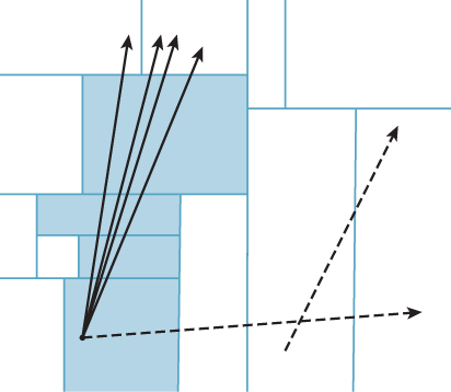
Figure 36.10: Packets of rays with similar direction and origin may perform similar traversals of a BSP tree. Processing them simultaneously on a parallel architecture can amortize the memory cost of fetching nodes and leverage vector registers and instructions. Rays that diverge from the common traversal (illustrated by dashed lines) reduce the efficiency of this approach.
Adding this kind of parallelism is more complicated than merely spawning multiple threads. It is also hard to ignore when considering high-performance visibility computations. At the time of this writing, vector instructions yield an 8x to 32x peak performance boost over scalar or branch-divergent instructions on the same processors. Fortunately, this kind of low-level visibility testing is increasingly provided by libraries, so you may never have to implement such an algorithm outside of an educational context. From a high level, one can look at hardware rasterization as an extreme optimization of parallel ray visibility testing for the particular application of primary rays under pinhole projection.
36.3. The Depth Buffer
A depth buffer [Cat74] is a 2D array parallel to the rendered image. It is also known as a z-buffer, w-buffer, and depth map. In the simplest form, there is one color sample per image pixel, and one scalar associated with each pixel representing some measure of the distance from the center of projection to the surface that colored the pixel.
To reduce the aliasing arising from taking a single sample per pixel, renderers frequently store many color and depth samples within a pixel. When resolving to an image for display, the color values are filtered (e.g., by averaging them), and the depth values are discarded. A variety of strategies for efficient rendering allow more independent depth samples than color samples, separating “shading” (color) from “coverage” (visibility). This section is limited to discussions of a single depth sample per pixel. We address strategies for multiple samples in Section 36.9.
Figure 36.11 reproduces Dürer’s etching of himself and an assistant manually rendering a musical instrument under perspective projection. We have seen and referred to this classic etching before. In it, one man holds a pen at the location where a string crosses the image plane to dot a canvas that corresponds to our color buffer. The pulley on the wall is the center of projection and the string corresponds to a ray of light. Now note the plumb bob on the other side of the pulley. It maintains tension in the string. Dürer’s primary interest was the 2D image produced by marking intersections of that string with the image plane. But, as we noted in Chapter 3, this apparatus can in fact measure more than just the image. Consider what would happen if the artist were to annotate each point he marked on the image plane with the length of string between the plumb bob and the pulley corresponding to that point. He would then record a depth buffer for the scene, encoding samples of all visible three-dimensional geometry.
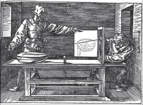
Dürer’s artist had little need of a depth buffer for a single image. The physical object in front of him ensured correct visibility. However, given two images with depth buffers, he could have composited them into a single scene with correct visibility at each point. At each sample, only the nearer depth value (which in this case means a longer string below the pulley) could be visible in the combined scene. Our rendering algorithms work with virtual objects and lack the benefit of automatic physical occlusion. For simple convex or planar primitives such as points and triangles we know that each primitive does not occlude itself. This means we can render a single image plus depth buffer for each primitive without any visibility determination. The depth buffer allows us to combine rendering of multiple primitives and ensure correct visibility at each sample point.
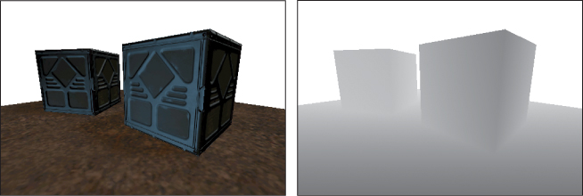
The depth buffer is often visualized with white values in the distance and black values close to the camera, as if black shapes were emerging from white fog (see Figure 36.12). There are many methods for encoding the distance. The end of this section describes some that you may encounter. Depth buffers are commonly employed to ensure correct visibility under rasterization. However, they are also useful for computing shadowing and depth-based post-processing in other rendering frameworks, such as ray tracers.
There are three common applications of a depth buffer in visibility determination. First, while rendering a scene, the depth buffer provides implicit visible surface determination. A new surface may cover a sample only if its camera-space depth is less than the value in the depth buffer. If it is, then that new surface overwrites the color in the depth buffer and its depth value overwrites the depth in the depth buffer. This is implicit visibility because until rendering completes it is unknown what the closest visible surface is at a sample, or whether a given surface is visible to the camera. Yet when rendering is complete, correct visibility is ensured.
Second, after the scene is rendered, the depth buffer describes the first scene intersection for any ray from the center of projection through a sample. Because the position of each sample on the image plane and the camera parameters are all known, the depth value of a sample is the only additional information needed to reconstruct the 3D position of the sample that colored it.
Third, after the scene is rendered, the depth buffer can directly evaluate the visibility function relative to the center of projection. For camera-space point Q, V((0, 0, 0), Q) = 1 if and only if the depth value at the projection of Q is less than the depth of Q.
The second and third applications deserve some more explanation of why one would want to solve visibility queries after rendering is already completed. Many rendering algorithms make multiple passes over the scene and the framebuffer. The ability to efficiently evaluate ray intersection queries and visibility after an initial pass means that subsequent rendering passes can be more efficient. One common technique exploiting this is the depth prepass [HW96]. In that pass, the renderer renders only the depth buffer, with no shading computations performed. Such a limited rendering pass may be substantially more efficient than a typical rendering pass, for two reasons. First, fixed-function circuitry can be employed because there is no shading. Second, minimal memory bandwidth is required when writing only to the depth buffer, which is often stored in compressed form [HAM06].
Note that a depth buffer must be paired with another algorithm such as rasterization for finding intersections of primary rays with the scene. Chapter 15 gives C++ code for ray casting and rasterization implementations of that intersection test. The rasterization implementation includes the code for a simple depth buffer. That implementation assumes that all polygons lie beyond the near clipping plane (see Chapter 13 for a discussion of clipping planes). This is to work around one of the drawbacks of the depth buffer: It is not a complete solution for visibility. Polygons need to be clipped against the near plane during rasterization to avoid the projection singularity at z = 0. The depth buffer can represent depth values behind the camera; however, rasterization algorithms are awkward and often inefficient to implement on triangles before projection. As a result, most rasterization algorithms pair a depth buffer with a geometric clipping algorithm. That geometric algorithm effectively performs a conservative visibility test by eliminating the parts of primitives that lie behind the camera before rasterization. The depth buffer then ensures correctness at the screen-space samples.
The depth buffer has proved to be a powerful solution for screen-space visibility determination. It is so powerful that not only has it been built in dedicated graphics circuitry since the 1990s, but it has also inspired many image-space techniques. Image space is a good place to solve many graphics problems because solving at the resolution of the output avoids excessive computation. In exchange for a constant memory factor overhead, many algorithms can run in time proportional to the number of pixels and sublinear to, if not independent of, the scene complexity. That is a very good algorithmic tradeoff. Furthermore, geometric algorithms are susceptible to numerical instability as infinitely thin rays and planes pass near one another on a computer with finite precision. This makes rasterization/image-space methods a more robust way of solving many graphics problems, albeit at the expense of aliasing and quantization in the result.
If there are T triangles in the scene and P pixels in the image, under what conditions on T and P would you expect image-space methods to be a good approach to visibility or related problems?
Image-space algorithms seem like a panacea. Describe a situation in which the discrete nature of image-space data makes it inappropriate for solving a problem.
36.3.1. Common Depth Buffer Encodings
Broadly speaking, there are two common choices for encoding depth: hyperbolic in camera-space z, and linear in camera-space z. Each has several variations for scaling conventions within the mapping. All have the property that they are monotonic, so the comparison z1 < z2 can be performed as m(z1) < m(z2) (perhaps with negation) so that the inverse mapping is not necessary to implement correct visibility determination.
There are many factors to weigh in choosing a depth encoding. The operation count of encoding and decoding (for depth-based post-processing) may be significant. The underlying numeric representation, that is, floating point versus fixed point, affects how the mapping ultimately reduces to numeric precision. The dominant factor is often the relative amount of precision with respect to depth. This is because the accuracy of the visibility determination provided by a depth buffer is limited by its precision. If two surfaces are so close that their depths reduce to the same digital representation, then the depth buffer is unable to distinguish which is closer to the ray origin or camera. This means that the visibility determination will be arbitrarily resolved by primitive ordering or by small roundoff errors in the intersection algorithm. The resultant artifact is the appearance of individual samples with visibility results inconsistent with their neighbors. This is called z-fighting. Often z-fighting artifacts reveal the iteration order of the rasterizer or other intersection algorithm, which tends to cause regular patterns of small bias in depth. Different mappings and underlying numerical representation for depth vary the amount of precision throughout the scene. Depending on the kind of scene and rendering application, it may be desirable to have more precision close to the camera, uniform precision throughout, or possibly even high precision at some specific depth. Akeley and Su give an extensive and authoritative treatment [AS06] of this topic. We summarize the basic ideas of the common mappings here and show Figures 36.13 and 36.14 by them to give a sense of the impact of representation on precision throughout the frustum.
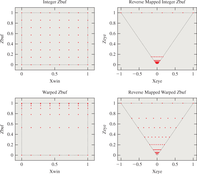
Figure 36.13: The points in (x, z bufferValue) space that are exactly representable under fixed-point, reverse-mapped fixed-point, and floating-point schemes. Fixed-point representations result in wildly varying depth precision with respect to screen-space x (or y).
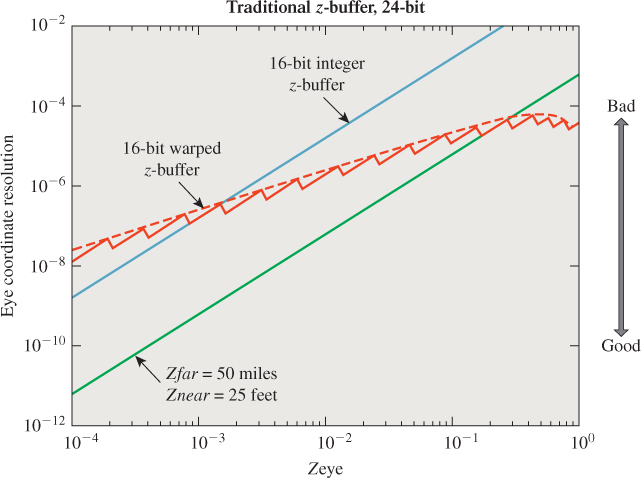
Figure 36.14: Comparison of precision versus depth for various z-buffer representations: 24-bit fixed point (green) is obviously strictly more accurate than 16-bit fixed point (blue); 16-bit floating point is more accurate than 16-bit fixed point when far from the camera (on the right), but has less precision very near to the camera (on the left). The blue and green curves are lines in log-log space, but would appear as hyperbolas in a linear plot. The red floating-point line is jagged because floating-point spacing is uniform within a single exponent and then jumps at the next exponent; the red curve is a smoothed trendline.
Following (arbitrary) OpenGL conventions, for the following definitions let z be the position on the camera-space z-axis of the point coloring the sample. It is always a negative value. Let the far and near clipping planes be at zf = −f and zn = − n.
36.3.1.1. Hyperbolic
The classic graphics choice describes a hyperbolically scaled normalized value arising from a projection matrix. This is typically called the z-buffer because it stores the z-component of points after multiplication by an API-specified perspective projection matrix and homogeneous division. This representation is also known as a warped z-buffer because it distorts world-space distances.
The OpenGL convention maps −n to 0, −f to 1, and values in between hyperbolically by
Direct3D maps to the interval [−1, 1] by
These mappings assign relatively more precision close to the near plane (where z-fighting artifacts may be more visible), have a normalized range that is appropriate for fixed-point implementation, and are expressible as a matrix multiplication followed by a homogeneous division. The amount of precision close to the near plane is based on the relative distance of the near and far planes from the center of projection. As the near plane moves closer to the center of projection, all precision rapidly shifts toward it, giving poor depth resolution deep in the scene.
A complementary or reversed hyperbolic [LJ99] encoding maps the far plane to the low end of the range and the near plane to the high end. For a fixed-point representation this is usually undesirable because nearby objects would receive higher depth representation errors, but under a floating-point representation this assigns nearly equal accuracy throughout the scene.
Another advantage of the nonlinear depth range is that it is possible to take the limit of the mapping as f ![]() ∞ [Bli93]. This allows a representation of depth within an infinite frustum using finite precision.
∞ [Bli93]. This allows a representation of depth within an infinite frustum using finite precision.
For n = 1m, f = 101m, compute the range of z-values within the view frustum that map to [0, 0.9] under the OpenGL projection matrix. Repeat the exercise for n = 0.1m. How would this inform your choice of near and far plane locations? What is the drawback of pushing the near plane farther into the scene?
This was the preferred depth encoding until fairly recently. It was preferred because it is mathematically elegant and efficient in fixed-function circuitry to express the entire vertex transformation process as a matrix product. However, the widespread adoption of programmable vertex transformations and floating-point buffers in consumer hardware has made other formats viable. This reopened a classic debate on the ideal depth buffer representation. Of course, the ideal representation depends on the application, so while this mapping may no longer be preferred for some applications, it remains well suited for others. More than storage precision is at stake. For example, algorithms that expect to read world-space distances from the depth buffer pay some cost to reconstruct those values from warped ones, and the precision of the world-space value and cost of recovering it may be significant considerations.
Linear The terms linear z, linear depth, and w-buffer describe a family of possible values that are all linear in z. The “w” refers to the w-component of a point after multiplication by a perspective projection matrix but before homogeneous division.
These representations include the direct z-value for convenience; the positive “depth” value –z; the normalized value (z + n)/(n – f) that is 0 at the near plane and 1 at the far plane; and 1 – (z + n)/(n – f), which happens to have nice precision properties in floating-point representation [LJ99]. In fixed point these give uniform world-space depth precision throughout the camera frustum, which makes z-fighting consistent in depth and can simplify the process of assigning decal offsets and other “epsilon” values. Linear depth is often conceptually (and computationally!) easier to work with in pixel shaders that require depth as an input. Examples include soft particles [Lor07] and screen-space ambient occlusion [SA07].
36.4. List-Priority Algorithms
The list-priority algorithms implicitly resolve visibility by rendering scene elements in an order where occluded objects have higher priority, and are thus hidden by overdraw later in the rendering process. These algorithms were an important part of the development of real-time mesh rendering.
Today list-priority algorithms are employed infrequently because better alternatives are available. Spatial data structures can explicitly resolve visibility for ray casts. For rasterization, the memory for a depth buffer is now fast and inexpensive. In that sense, brute force image-space visibility determination has come to dominate rasterization. But the depth buffer also supports an intelligent algorithmic choice. Early depth tests and early depth rendering passes avoid the inefficiency of overdrawing samples, and today’s renderers spend significantly more time shading samples than resolving visibility for them because shading models have grown very sophisticated. So a list-priority visibility algorithm that increases shading time is making the expensive part of rendering more expensive. Despite their current limited application, we discuss three list-priority algorithms.
However, the implicit and refreshingly simple approach of implicit visibility by priority is a counterpoint to the relative complexity of something like hierarchical occlusion culling. There are also some isolated applications, especially graphics for nonraster output, where list priority may be the right approach. We find that the painter’s algorithm is embedded in most user interface systems, and is often encountered even in sophisticated 3D renderers for handling issues like transparency when memory or render time is severely limited.
Some list-priority algorithms are heuristics that often generate a correct ordering, but fail in some cases. Others produce an exact ordering, which may require splitting the input primitives to resolve cases such as Figure 36.15. There’s an important caveat for the algorithms that produce exact results: If we are going to do the work of subdivision, we can achieve more efficient rendering by simply culling all occluded portions, rather than just overdrawing them later in rendering. This was a popular approach in the 1970s. Area-subdivision algorithms such as Warnock’s Algorithm [War69] and the Weiler-Atherton Algorithm [WA77] eliminate culled areas in 2D. There are similar per-scanline 1D algorithms such as those by Wylie et al. [WREE67], Bouknight [Bou70], Watkins [Wat70], and Sechrest and Greenberg [SG81] that use an active edge table to maintain the current-closest polygon along a horizontal line. These were historically extended to single-line depth buffers [Mye75, Cro84]. The obvious trend ensued, and today all of these are largely ignored in favor of full-screen depth buffers. This is a cautionary tale for algorithm development in the long run, since the simplicity found in the depth buffer and painter’s algorithm leads to better performance and more practical implementation than decades of sophisticated visibility algorithms.
36.4.1. The Painter’s Algorithm
Consider a possible process for an artist painting a landscape. The artist paints the sky first, and then the mountains occluding the sky. In the foreground, the artist paints trees over the mountains. This is called the painter’s algorithm in computer graphics. Occlusion and visibility are achieved by overwriting colors due to distant points with colors due to nearer points. We can apply this idea to each sample location because at each sample there is always a correct back-to-front ordering of the points directly affecting it. In this case, the algorithm is potentially inefficient because it requires sorting all of the points, but it gives a correct result.
For efficiency, the painter’s algorithm is frequently applied to whole primitives, such as triangles. Here it fails as an algorithm. While primitives larger than points can often be ordered so as to give correct visibility, there are situations where this cannot be done. Figure 36.15 shows three triangles for which there is no correct back-to-front order. Here the “algorithm” is merely a heuristic, although it can be an effective one. If we allow subdividing primitives where their projections cross, then we can achieve an ordering. This is discussed in the following section.
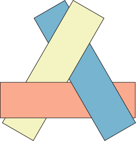
Figure 36.15: Three convex polygons that cannot be rendered properly using the painter’s algorithm due to their mutual overlaps. At each point, a strict depth ordering exists, but there is no correct ordering of whole rectangles.
Despite its inability to generate either correct or conservative results in the general case, the painter’s algorithm is employed for some niche applications in computer graphics and is a useful concept in many cases. It is trivially simple, requires no space, and can operate out of core (provided the sort is implemented out of core). It is the predominant visibility algorithm in 2D user interfaces and presentation graphics. In these systems, all objects are modeled as lying in planes parallel to the image plane. For that special case, the primitives can always be ordered, and the ordering is trivial to achieve because those planes are typically parallel to the image plane.
When we render with a depth buffer and an early depth test, it is advantageous to encounter proximate surfaces before distant ones. Distant surfaces will then fail the early depth test where they are occluded, and not require shading. A reverse painter’s algorithm improves efficiency in that case: Render from front to back. A depth prepass eliminates the need for ordering. During the prepass itself the ordering provides a speedup. Surprisingly, for many models a static ordering of primitives can be precomputed that provides a good front-to-back ordering from any viewpoint [SNB07]. This allows the runtime performance without the runtime cost.
The painter’s algorithm is often employed for translucency, which can be modeled as fractional visibility values between zero and one, as done in OpenGL and Direct3D. Compositing translucent surfaces from back to front allows a good approximation of their fractional occlusion of each other and the background in many cases. However, stochastic methods yield more robust results for this case at the expense of noise and a larger memory footprint. See Section 36.9 for a more complete discussion.
36.4.2. The Depth-Sort Algorithm
Newell et al.’s depth-sort algorithm [NNS72] extends the painter’s algorithm for polygons to produce correct output in all cases. It operates in four steps.
1. Assign each polygon a sort key equal to the camera-space z-value of the vertex farthest from the viewport.
2. Sort all polygons from farthest to nearest according to their keys.
3. Detect cases where two polygons have ambiguous ordering. Subdivide such polygons until the pieces have an explicit ordering, and place those in the sort list in the correct priority order.
4. Render all polygons in priority order, from farthest to nearest.
The ordering of two polygons is considered ambiguous under this algorithm if their z-extents and 2D projections (i.e., their homogeneous clip-space, axis-aligned bounding boxes) overlap and one polygon intersects the plane of the other.
36.4.3. Clusters and BSP Sort
Consider a scene defined by a set of polygons and a viewer using a pinhole projection model. Schumacker [SBGS69] noted that a plane passing through the scene that does not intersect any polygons divides them into two sets. Those polygons on the same side of the plane as the viewer must be strictly closer to the viewer, and thus cannot be occluded by those polygons on the farther side. He grouped polygons into clusters, and recursively subdivided them when suitable partition planes could not be found. Within each cluster he precomputed a viewer-independent ordering (see later work by Sander et al. [SNB07] on a related problem), and employed a special-purpose rasterizer that followed these orderings.
Fuchs, Kedem, and Naylor [FKN80] generalized these ideas into the binary space partition tree. We have already discussed in this chapter how BSP trees can solve visible surface determination by accelerating ray-primitive intersection. They can also be applied in the context of a list-priority algorithm, and that was their original motivating application. (We will shortly see two more applications of BSP trees to visibility: portals and mirrors, and precomputed visibility.)
The same logic found in the ray-intersection algorithm applies to the list-priority rendering with a BSP tree; we are conceptually performing ray intersection on all possible view rays. Listing 36.2 gives an implementation that sorts all polygons from farthest to nearest, given a previously computed BSP tree. We can look at this as a variation on the depth-sort algorithm where we are guaranteed to never encounter the case requiring subdivision. We never need to subdivide during traversal because the tree’s construction already performed subdivision at partition planes between nearby polygons.
Listing 36.2: The list-priority algorithm for rendering polygons in a BSP tree with root node as observed by a viewer at P.
1 function BSPPriorityRender(P, node):
2 if node is a leaf:
3 render the polygon at node
4 return
5
6 closer = node.positiveChild
7 farther = node.negativeChild
8
9 if P is in the negative half-space of node:
10 swap closer, farther
11
12 BSPPriorityRender(P, farther)
13 BSPPriorityRender(P, closer)
36.5. Frustum Culling and Clipping
Assume that we rely on an exact method like a depth buffer or Newell et al.’s depth-sort algorithm for correct visibility under rasterization. To avoid writing to illegal or incorrect memory addresses, assume that we perform 2D scissoring to the viewport. This just means that the rasterizer may generate (x, y) locations that are outside the viewport, but we only allow it to write to memory at locations inside the viewport. We can also scissor in depth: No sample may be written whose depth indicates that it is behind the camera or past the far plane.
Recall that Chapter 13 showed that a rectangular viewport with near and far planes parallel to the image plane defines a volume of 3D space called the view frustum. This is a pyramid with a rectangular base and the top cut off. Clipping to the sides of the view frustum in 3D corresponds to clipping the projection of primitives to the viewport, and produces equivalent results to simply scissoring in 2D.
Scissoring alone ensures correctness, but it may lead to poor efficiency. For example, most primitives that are rasterized may fail the scissor test. There are three common approaches to increasing efficiency in this case that are related to the view frustum.
• Frustum culling: Eliminate polygons that are entirely outside the frustum, for efficiency.
• Near-plane clipping: Clip polygons against the near plane to enable simpler rasterization algorithms and avoid spending work on samples that fail depth scissoring.
• Whole-frustum clipping: Clip polygons to the side and far planes, for efficiency.
In general, it is a good strategy to use scissoring and clipping to complement each other. Use each only for the case where it has high efficiency and low implementation complexity. For example, use a coarse culling based on the view frustum followed by clipping to the near plane and scissoring in 2D. For primitives whose projections are small compared to the viewport, this leads to the scissor test usually passing, which means that most parts of most rasterized primitives for which significant computation is performed are usually on the screen.
36.5.1. Frustum Culling
Eliminating polygons outside the view frustum is simple. One 3D algorithm for this tests each vertex of a polygon against each plane bounding the view frustum. Assume that the planes are oriented so that the view frustum is the intersection of the six positive half-spaces. If there exists some plane for which all vertices of a polygon are in the negative half-space, then that polygon must lie entirely outside the view frustum and can be culled. For small polygons, it may not be efficient to perform this test on each polygon. For example, if a polygon affects at most one sample, then a 3D bounding box test on a single point yields the same result. So frustum culling may be performed on a bounding box hierarchy.
A drawback of the 3D frustum culling algorithm just described is that it may be too conservative. Polygons that are outside the view frustum but near a corner or edge may intersect multiple planes.
36.5.2. Clipping
36.5.2.1. Sutherland-Hodgman 2D Clipping
There are many clipping algorithms. Perhaps the simplest is the 2D variation of Sutherland’s and Hodgman’s [SH74] algorithm. It clips one (arbitrary) source polygon against a second, convex boundary polygon (see Figure 36.16). The algorithm proceeds by incrementally clipping the source against the line through each edge of the boundary polygon, as shown in Listing 36.3.
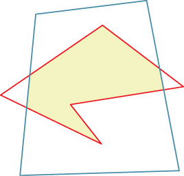
Figure 36.16: The red input polygon is clipped against the convex blue boundary polygon; the result is the boundary of the yellow shaded area.
Construct an example input polygon which, when clipped against the unit square by the Sutherland-Hodgman algorithm, produces a polygon with degenerate edges (i.e., edges that meet at a vertex v with an exterior angle of 180°).
For viewport clipping, Sutherland-Hodgman is applied to a projected polygon and the rectangle of the viewport. For projected polygons that have significant area outside the viewport, clipping to the viewport is an efficient alternative to scissor-testing each sampled point. The algorithm is further useful as a general geometric operation in many contexts, including modeling shapes in the first place.
Listing 36.3: Pseudocode for Sutherland-Hodgman clipping in 2D.
1 // The arrays are the vertices of the polygons.
2 // boundaryPoly must be convex.
3 function polyClip(Point sourcePoly[], Point boundaryPoly[]):
4 for each edge (A, B) in boundaryPoly:
5 sourcePoly = clip(sourcePoly, A, Vector(A.y-B.y, B.x-A.x))
6 return sourcePoly
7
8 // True if vertex V is on the "inside" of the line through P
9 // with normal n. The definition of inside depends on the
10 // direction of the y-axes and whether the winding rule is
11 // clockwise or counter-clockwise.
12 function inside(Point V, Point P, Vector n):
13 return (V - P).dot(n) > 0
14
15 // Intersection of edge CD with the line through P with normal n
16 function intersection(Point C, Point D, Point P, Vector n):
17 distance = (C - P).dot(n) / n.length()
18 t = (D - C).length()
19 return D* t + C* (1 - t)
20
21 // Clip polygon sourcePoly against the line through P with normal n
22 function clip(Point sourcePoly[], Point P, Vector n):
23 Point result[];
24
25 // Add the last point, if it is inside
26 D = sourcePoly[sourcePoly.length - 1]
27 Din = inside(D, P, n)
28 if (Din): result.append(D)
29
30 for (i = 0; i < sourcePoly.length; ++i) :
31 C = D, Cin = Din
32
33 D = sourcePoly[i]
34 Din = inside(D, P, n)
35
36 if (Din != Cin): // Crossed the line
37 result.append(intersection(C, D, P, n))
38
39 if (Din): result.append(D)
40
41 return result
The algorithm produces some degenerate edges, which don’t matter for polygon rasterization but can cause problems when we apply the same ideas in other contexts.
36.5.2.2. Near-Plane Clipping
The 2D Sutherland-Hodgman algorithm generalizes to higher dimensions. To clip a polygon to a plane, we walk the edges finding intersections with the plane. We can do this for the whole view frustum, processing one plane at a time. Consider just the step of clipping to the near plane for now, however.
In camera space, the intersections between polygon edges and the near plane are easy to find because the near plane has a simple equation: z = –n. In fact, this is exactly the same problem as clipping a polygon by a line, since we can project the problem orthogonally into either the xz- or yz-plane. We interpolate vertex attributes that vary linearly across the polygon linearly to the new vertices introduced by clipping, as if they were additional spatial dimensions. Listing 36.4 gives the details in pseudocode for clipping a polygon specified by its vertex list against the plane z = zn, where zn < 0.
Listing 36.4: Clipping of the polygon represented by the vertex array against the near plane z = zn.
1 function clipPolygon(inVertices, zn):
2 outVertices = []
3 Let start = inputVertices.last();
4 for end in inputVertices:
5 if end.z <= zn:
6 if start.z > zn:
7 // We crossed into the frustum
8 outVertices.append( clipLine(start, end, zn) )
9
10 // the endpoint of this edge is in the frustum
11 outVertices.append( end )
12
13 elif start.z <= zn:
14 // We crossed out of the frustum
15 outVertices.append( clipLine(start, end, zn) )
16
17 start = end
18
19 return outVertices
20
21
22 function clipLine(start, end, zn):
23 a = (zn - start.z) / (end.z - start.z)
24 // This holds for any vertex properties that we
25 // wish to linearly interpolate, not just position
26 return start * a + end * (1 - a)
36.5.3. Clipping to the Whole Frustum
Having clipped against the near plane, we are guaranteed that for every vertex in the polygon z < 0. This means that we can project the polygon into homogeneous clip space, mapping the frustum to a cube through perspective projection as described in Chapter 13.
We could continue with Sutherland-Hodgman clipping for the other frustum planes in 3D before projection. However, the side planes are not orthogonal to an axis the way that the near plane is, so clipping to those planes takes more operations per vertex. In comparison, after perspective projection every frustum plane is orthogonal to some axis, so clipping is just as efficient for a side plane as it was for the near plane. That is, clipping is again a 2D operation. Clipping to the far plane can be performed either before or after projection.
When clipping in Cartesian 3D space against the near plane, we were able to linearly interpolate per-vertex attributes such as texture coordinates. In homogeneous clip space, those attributes do not vary linearly along an edge, so we cannot directly linearly interpolate. However, the relationship is nearly as simple.
In practice, we don’t need all of those operations for each edge clipping operation. Instead, we can project every attribute by u′ = –u/z when projecting position. Then we can perform all clipping on the u′ attributes as if they were linear and all operations were 2D. Recall that rasterization needs to interpolate attributes in a perspective-correct fashion, so it operates on the u′ attributes along a scan line anyway (see The Depth Buffer). Only at the per-sample “shading” step do we return to the original attribute space, by computing u = –u′z with the hyperbolically interpolated z-value. Thus, in practice, the clipping (and rasterization) cost for 3D attributes is the same as for 2D attributes, and all of the 2D optimization techniques such as finite differences can be applied to the u′-values.
36.6. Backface Culling
The back of an opaque, solid object is necessarily hidden from direct line of sight from an observer. The object itself occludes the view rays. Culling primitives that lie on the backs of objects can therefore conservatively eliminate about half of the scene geometry. As pointed out previously, backface culling is a good optimization when computing the visibility function, but not for the entire rendering pipeline. When we consider the entire rendering pipeline, the image may be affected by points not directly visible to the camera, such as objects seen by their reflections in mirrors and shadows cast by objects outside the field of view. So, while backface culling is one of the first tools that we reach for when optimizing visibility, it is important to apply it at the correct level. One can occasionally glimpse errors arising from programs culling at the wrong stage, such as shadows disappearing when their caster is not in view.
Although backface culling could be applied to parametric curved surfaces, it is typically performed on polygons. That is because a test at a single point on the polygon indicates whether the entire polygon lies on the front or back of an object, so it is very efficient to test polygons. A curve may require tests at multiple points or an analytic test over the entire surface to make the same determination.
We intuitively recognize the back of an object—it is what we can’t see!—but how can we distinguish it geometrically? Consider a closed polygonal mesh with no self-intersections, and an observer at point Q that lies outside the polyhedron defined by the mesh. Let P be the vertex of a polygon and ![]() be the normal to the polygon (specifically, the true geometric normal to the polygon, not some implied surface normal at the vertex to be used in smooth shading). The polygon defines a plane that passes through P and has normal
be the normal to the polygon (specifically, the true geometric normal to the polygon, not some implied surface normal at the vertex to be used in smooth shading). The polygon defines a plane that passes through P and has normal ![]() . We say that the polygon is a frontface with respect to Q if Q lies in the positive half-plane of the polygon and that the polygon is a backface if Q lies in the negative half-plane. If Q lies exactly in the plane, then the polygon lies on the contour curve dividing the front and back of the object.
. We say that the polygon is a frontface with respect to Q if Q lies in the positive half-plane of the polygon and that the polygon is a backface if Q lies in the negative half-plane. If Q lies exactly in the plane, then the polygon lies on the contour curve dividing the front and back of the object.
The result will be the same for the polygon regardless of which vertex we choose for a polygon, and regardless of the field of view of the camera. However, Figure 36.17 shows that an object close to the camera tends to have more backfaces than the same object far from the camera, and that this is a general phenomenon, at least for convex objects.
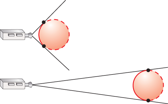
Figure 36.17: Two cameras facing to the right, toward spheres. The long lines depict the rays from the center of projection to the silhouette of the sphere, which is where the backfacing and frontfacing surfaces meet. The top camera is near a sphere, so most of the sphere’s surface is backfacing. The bottom camera is distant from its sphere, so only about half of the sphere’s surface is backfacing.
Prove that for a triangle and a viewer, the backface classification is independent of which vertex we consider.
Most ray tracers and rasterizers perform backface culling on whole triangles before progressing to per-sample intersection tests. This is a more effective strategy for rasterizers because they can amortize the backface test (and the corresponding cost of reading the triangle into memory) over the whole triangle. A ray tracer generally must perform the test once per sample.
Backface culling assumes opaque, solid objects. If the ray starting point Q (e.g., the viewpoint for a primary ray) is inside the volume bounded by a mesh, then it is not conservative to cull backfaces. It also isn’t obvious what the result of visibility determination should be in such a situation because it does not correspond to a physically plausible scene. If an object is composed of a material that transmits light, then a geometric “visibility” test does not correspond to a light transport visibility test.
If we abuse geometric visibility in this case and apply backface culling, the back surface will disappear. In practice one can model a transmissive object with coincident and oppositely oriented surfaces. For example, a glass ball consists of a spherical air-glass interface oriented outward from the center of the ball and a glass-air interface oriented inward. Backface culling remains conservative under this model. Along a path that does not experience total internal refraction, light originating outside the ball first interacts with an air-glass frontface to enter the ball and then with a glass-air frontface to exit again, as shown in Figure 36.18.
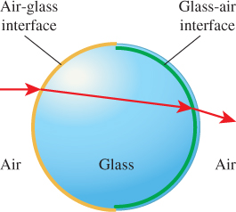
Figure 36.18: Backface culling allows a ray to intersect the correct one of the two coincident air-glass and glass-air interfaces of a glass ball surrounded by air.
36.7. Hierarchical Occlusion Culling
If no part of a box is visible from a point Q that is outside of the box, and if the box is replaced with some new object that fits inside it, then no part of that object can possibly be visible either. This observation holds for any shape, not just a box. This is the key idea of occlusion culling. It seeks to conservatively identify that a complex object is not visible by proving that a geometrically simpler bounding volume around the object is also not visible. It is an excellent strategy for efficient conservative visibility determination on dynamic scenes.
How much simpler should the bounding volume be? If it is too simple, then it may be much larger than the original object and will generate too many false-positive results (i.e., the bounding volume will often be visible even when the actual object is not). If it is too complex, then we gain little net efficiency even if it is a good predictor. The natural solution is to divide and conquer. Create a Bounding Volume Hierarchy (BVH; see Chapter 37) and walk its tree. If a node is not visible, then all of its children must not be visible. This is one form of hierarchical occlusion culling.
A ray tracer with a hierarchical spatial data structure effectively performs occlusion culling, although the term is not typically applied to that case. For example, a ray cast through a BVH corresponds exactly to the algorithm from the previous paragraph.
For rasterization, occlusion culling is only useful if we can test visibility for the bounding volumes substantially faster than we can for the primitives themselves. There are two implementation strategies, commonly built directly into rasterization hardware, that support this.
The first is a special rasterization operation called an occlusion query [Sek04] that invokes no shading or changes to the depth buffer. Its only output is a count of the number of samples that would have passed the depth buffer visibility test. It can be substantially faster than full rasterization because it requires no output bandwidth to the framebuffer and no synchronous access to the depth buffer for updates, interpolates no attributes except depth, and launches no shading operations. Chapter 38 shows that those are often the expensive operations in rasterization, so eliminating them decreases the cost of rasterization substantially.
Occlusion culling with an occlusion query issues several queries asynchronously from the main rendering thread. When the result of a query is available, it then renders the corresponding object if and only if one or more pixels passed the occlusion query. This is made hierarchical by recursively considering bounds on smaller parts of the scene when a visible bound is observed.
The second strategy for efficient hardware occlusion culling is the hierarchical depth buffer, a.k.a. hierarchical z-buffer [GKM93]. This is an image pyramid similar to a MIP map in depth. Level zero of the tree is the full-resolution depth buffer. Every subsequent level has half the resolution of its parent level. A sample in level k + 1 of the hierarchical depth buffer stores two values: the minimum and maximum depths of four corresponding samples from level k. A hierarchical rasterizer [GKM93, Gre96] working with such a structure solves for minimum (or maximum, depending on the desired depth test) depth of a primitive within the area surrounding each of the depth samples at the lowest resolution. If the primitive’s minimum depth is smaller (i.e., closer to the camera) than the maximum depth at a sample, then some part of that primitive may be visible at the highest resolution, so the rasterizer progresses to the next level for that sample. If the primitive’s minimum depth is greater than or equal to the maximum depth at a depth buffer sample, then even the farthest point in the subtree represented by that sample is still closer to the camera than the closest point on the primitive and the primitive must be occluded at all resolutions represented.
A hierarchical depth buffer is naturally most efficient for large primitives. This is because because when parts of a large primitive are conservatively classified as invisible near the top of the tree, many high-resolution visibility tests are eliminated. Small primitives force the rasterizer to begin tests deeper in the tree where the potential cost savings are smaller. Because hierarchical occlusion queries on BVHs tend to bound meshes of small primitives with a few large ones, they benefit from both the occlusion query and the improved hierarchical depth buffer efficiency. Thus, the “hierarchical” in hierarchical occlusion query often refers to both the image-space depth buffer tree and the geometric bounding volume tree.
36.8. Sector-based Conservative Visibility
In this section we explore alternative uses of the spatial partitioning created by the partition operations that occur when building a BSP tree. These techniques, especially stabbing trees, were critical for real-time rendering of indoor environments from the early 1990s through the 2000s. They contain some beautiful computer science and geometric ideas. However, at the time of this writing they are passing out of favor because hierarchical occlusion culling allows more flexibility for managing dynamic and arbitrarily shaped environments. Although these algorithms can be applied for explicit point-to-point visibility tests, they are typically used to generate a potentially visible set (PVS) of primitives for a given viewpoint.
Recall that the leaves of a BSP tree are polygons that have been repeatedly clipped against planes, at least for the version that we have discussed in this chapter. If we assume that the original polygons, before all of the subdivision, were convex and planar, then the leaves must also be convex and planar.
Any point in space can be classified by some path through the tree, corresponding to whether it is in the positive or negative half-space of each node’s splitting plane. That series of planes carves space into a convex polyhedron that contains the point. The space inside this polyhedron is called a sector. The polyhedron may have infinite volume if the point is near the edge of the scene.
Some of the faces of a sector correspond to leaves in the BSP tree. These polygons block visibility. Others are empty space. Those are called portals because they are windows to adjacent sectors. A convex space has a nice visibility property: All points within the space are visible to all other points. (For a pinhole camera, one may choose to then restrict that visibility by the field of view to the image frame.) From any point in a sector, one can look through any portal into any adjacent sector. However, in doing so, our visibility within the adjacent sector is restricted to a frustum that is the extrusion of the portal’s boundary away from the viewer. If we look straight through a sector into another sector through a second portal, visibility becomes restricted by the intersection of the two portals’ extrusions. After many portals, this frustum can become small; if one portal lies outside the frustum of another, the intersection of their frusta is empty. Most of these key observations are due to Jones [Jon71] and form a family of visibility determination algorithms.
Consider the graph in which sectors are nodes and portals are edges. A point is visible to another point only if it is reachable in this graph. Furthermore, we can detect cases where the specific geometry of adjacent sectors prevents looking straight through more than two portals. For example, in a grid of nonrefractive and nonreflective windows, we can look through a window to our north into an adjacent sector and then through its east window into another one; but we cannot look through that sector’s south window because that would require bending a viewing ray into an arc. This corresponds to the case of the third sector’s south window lying entirely outside the intersection for the frusta of the first two.
For an interesting scene there might be a tremendous number of sectors, so following the graph line of thinking might be inefficient. But if we exclude small objects such as furniture from the sector-building algorithm and only consider large objects such as walls when building sectors and portals, we may find a relatively small number of sectors [Air90]. Any approach to visibility computation that ignores the so-called small detail objects only provides conservative visibility, and must be succeeded by another algorithm for correctness—the depth buffer is a common choice here.
Explicitly, V(P, Q) must be zero if no part of the sector containing point P is visible to the sector containing Q. Given some algorithm for determining sector-to-sector visibility, we can then conservatively approximate point and primitive visibility. Airey [Air90] pioneered a number of sector-to-sector visibility algorithms including ray casting and shadow volumes. The methods that he described are all correct with high probability for large numbers of samples, but are not all conservative; thus, the net visibility computation is not conservative under those approaches.
36.8.1. Stabbing Trees
Teller [Tel92] devised a closed-form, conservative, analytic algorithm for conservative visibility between sectors. His algorithm computes a BSP tree on n polygons in O(n2) operations to form the sectors. It then computes all possible straight-line stabbing line traversals through the sector adjacency graph until occlusion in worst-case O(n3) time, using a linear programming optimization framework. The full set of traversals from one sector is called a stabbing tree. In practice, the O(n3) asymptotic bound is misleading. There are many trivial rejection cases, such as when a portal is a backface to the viewer, and the constant factors are fairly small. Teller observed O(n) behavior in practice on complex indoor models. Nonetheless, the latter step must be performed for each pair of sectors, so the entire algorithm is slow enough to be an offline process that may take minutes or hours. When the algorithm terminates, each sector is annotated with a list of all other sectors that are conservatively visible to it.
At runtime in Teller’s framework, a point in space is associated with a sector by walking the original BSP tree in typically O(log n) time. That sector then provides its list of all potentially visible sectors, which quickly culls most of the scene geometry. Individual point-to-point visibility tests by ray casting can then be performed for explicit visibility tests. Alternatively, all polygons (including detail objects) in the potentially visible sectors can be rasterized with a depth buffer for implicit visibility during rendering. The latter approach was introduced in the Quake video game in 1996 and quickly spread throughout the game industry.
36.8.2. Portals and Mirrors
Teller’s stabbing trees require a long precomputation step that precludes their application to scenes with dynamic (nondetail) geometry. The Portals and Mirrors algorithm [LG95] is an alternative. It is simpler to implement and extends to both dynamic scenes and a notion of indirect visibility through mirrors. It revisits the frustum created when looking through a portal, but in the absence of the BSP tree and in the case where sectors may be nonconvex. That allows the sector geometry to change at runtime. The idea of the algorithm is to recursively trace the view frustum through portals, clipping it to each portal traversed. Figure 36.19 shows two visualizations of the algorithm. The first image is the camera’s view, with clipping regions at portals and mirrors highlighted. The second image is a top view of the scene, showing how the frustum shrinks as it passes through successive portals and reflects when it hits a mirror.
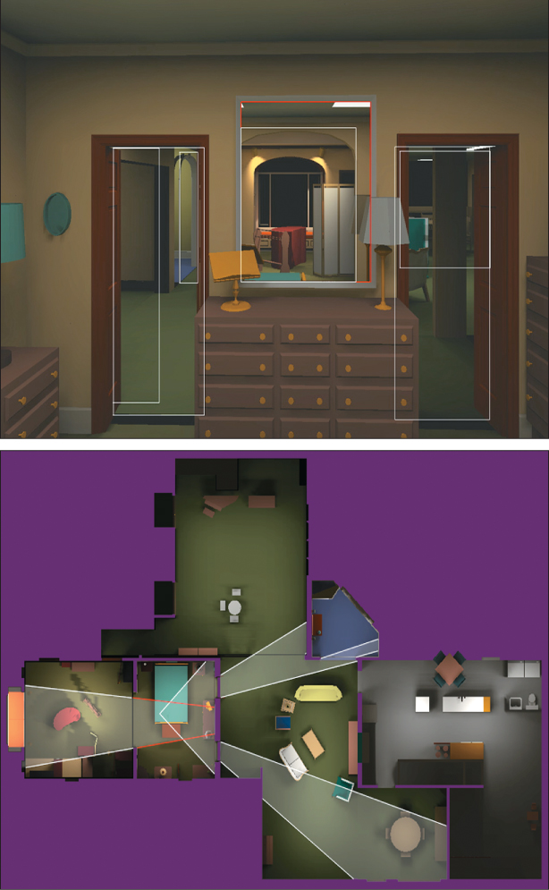
Figure 36.19: (Top) View inside Fred Brooks’ bedroom. There are two open doors and a mirror between them. The resultant portals are outlined in white and the mirrors are outlined in red. (Bottom) Schematic of visible regions for the observer from the top image. Note how the sight lines to the mirror give rise to a reflected visibility frustum that passes behind the viewer. (Courtesy of David Luebke ©1995 ACM, Inc. Reprinted by permission.)
Let the scene be represented as the sector polyhedra, the adjacency information between them, and the detail objects. Assume that at the beginning of an interactive sequence we know which sector contains the viewer, and that the viewer must move continuously through space (i.e., no teleportation!). Whenever the viewer moves through a portal, update the viewer state to retain a pointer to the sector that now contains the center of projection by following the adjacency information associated with that portal. This allows identifying the viewer’s sector in O(1) time during any frame.
To render a frame, let clipPoly initially be the screen-space rectangle bounding the viewport and sector be the viewer’s current sector. Invoke the portalRender(sector, clipPoly) function from Listing 36.5. It will recursively render objects seen through portals, recursing when there are no new portals that can be seen. The intersect routine is simply 2D convex polygon-polygon intersection, which can be performed using the Sutherland-Hodgman algorithm.
For a scene in which the sectors are convex and there is no detail geometry, this algorithm provides exact visibility—no depth buffer is needed. A strength of the method is that if we do use a depth buffer, not only can it accommodate nonconvex portals and detail geometry, but also the general 2D clipping can be replaced with conservative rectangle clipping on the bounding box of projPoly. This may trigger a few extra recursive calls, but it dramatically simplifies the clipping/intersection process because we need only work with screen-space, axis-aligned rectangles.
The extension to mirrors is conceptually straightforward. We can model a mirror as a portal to a virtual world that resembles the real world but is flipped left-to-right. To implement this, augment portalRender to track whether the viewpoint has been reflected through an even or odd number of mirrors, and reflect the viewer through the plane of the mirror. Two complications of the mirrors are that they must lie on the faces of a sector (i.e., they cannot be detail polygons) and that for a nonconvex sector, care must be taken not to reflect geometry that is behind the mirror in front of it in the virtual world. That is, the virtual world seen through the mirror must be clipped against the plane of the mirror, until the next mirror is encountered. The issues that arise in this case are analogous to those for stencil-masked mirrors; see Kilgard’s technical report [Kil99] for an explanation of how to perform the clipping and reflect the projection matrix.
Listing 36.5: Portal portion of the Portals and Mirrors algorithm.
1 function portalRender(sector, clipPoly):
2 render all detail objects in sector
3
4 for each face F in sector:
5 if F is not a backface:
6 if F is a portal:
7 // Limit visibility by the bounds of the portal
8 projPoly = project( clipToNearPlane(F.polygon) )
9 newClip = intersect( projPoly, clipPoly )
10
11 if newClip is not empty:
12 portalRender( F.nextSector, newClip )
13 else:
14 // F is an opaque wall
15 render F.polygon
36.9. Partial Coverage
There are several situations in which it is useful to extend binary visibility, also known as binary coverage, to partial coverage values on the interval [0, 1]. Many of these relate to the imaging model.
Consider the imaging model under which we defined binary coverage. For a pinhole camera with an instantaneous shutter there is a single ray that can transport light to each point on the image plane. The scene does not move relative to the camera because the exposure time is zero. At a single point Q on the image plane we can thus directly apply the binary visibility function to a point P in the scene.
Now consider a physically based lens camera model that has a nonzero shutter time and pixels of nonzero area. The radiant energy measured by a pixel in an image is an integral of the incident radiance function over the area of the pixel, solid angle subtended by the aperture, and exposure time. This creates a set of five parameters, sometimes labeled (x, y, u, v, t), that identify the path from a point Q′(x, y, u, v, t) on the image plane through the lens to a point P′ (t) in the scene. We introduce the primes to distinguish these from the points with which we have previously been concerned.
The binary visibility function between points on P′ and Q′ may vary with the parameters. The partial coverage (a.k.a. coverage) of points in the set P′(t) from points in the set Q′(x, y, u, v, t) is the integral of the binary visibility function over all parameter variations within the domain of those sets. As the area-weighted average of binary visibility, partial coverage values are necessarily on the range [0, 1]. To extend the definition to whole surfaces, we can consider points on a surface P′(i, j, t) parameterized by both surface location (i, j) and time t.
36.9.1. Spatial Antialiasing (xy)
Visibility under instantaneous pinhole projection, and thus coverage as well, between points P and Q is a binary value. However, coverage between a set of points in the scene and a set of points on the image plane can be fractional, since those sets give rise to many possible rays that may have different binary visibility results.
Of particular interest is the case where the region in the scene is a surface defined by values of the function P′(i, j, t)—a moving patch—and the region on the image plane is a pixel. For simplicity in definitions, assume the surface is a convex polygon so that it cannot occlude itself. We say that a surface defined by P′(i, j, t) fully covers the pixel when the binary visibility function to all points of the form Q(x, y, u, v, t) is 1 for all parameters. We say that the surface partially covers the pixel if the integral of the binary visibility function over the parameter space is less than 1.
Aliasing is, broadly speaking, caused by trying to store too many values in too few slots (see Figure 36.21 and Chapter 18). As in a game of musical chairs, some values cannot be stored. Aliasing arises in imaging when we try to represent all of the light from the scene that passes through a pixel using a single sample point (e.g., the one in the center). In this case, a single, binary visibility value represents the visibility of the whole portion of the surface that projects within the pixel area. The single sample covers infinitesimal area. Over that area, the binary visibility result is in fact accurate. But the pixel’s area2 is much larger, so the binary result is insufficient to represent the true coverage—there may be only fractional coverage. Rounding that fractional coverage to 0 or 1 creates inaccuracies that often appear in the form of a blocky image. Introducing a better approximation of partial coverage that considers multiple light paths can reduce the impact of this artifact. The process of considering more paths (or equivalently, samples) is thus called antialiasing.
2. More precisely: the support of the measurement or response function for the pixel.
Ideally, we’d integrate the incident radiance function over the entire pixel area, or perhaps the support of a sensor-response function, which may be larger than a pixel. For now, let’s assume that pixels respond only to light rays that pass through their bounds and have uniform response regardless of where within the pixel we sample the light.
Some definitions will maintain precise languages when we distinguish between the value of a pixel and a value at a point within the pixel. Figure 36.20 shows a single primitive (a triangle) overlaid on a pixel grid. A fragment is the part of a pixel that lies within a given pixel. Each pixel contains one or more samples, which correspond to primary rays. To produce an image, we need to compute a color for each pixel. This color is computed from values at each sample. The samples, however, need not be computed independently. For example, all of the samples in the central pixel are completely covered by one fragment, so perhaps we could compute a single value and apply it to all of them. We refer to the process of computing a value for one or more samples as shading, to distinguish it from computing coverage, that is, which samples are covered by a fragment. Although our discussion has been couched in the language of physically based rendering, “shading” applies equally well to arbitrary color computations (e.g., for text or expressive rendering).
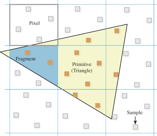
Figure 36.20: A pixel is a rectangular region of the framebuffer. A primitive is the geometric shape to be rendered, such as a triangle. A fragment is the portion of a primitive that lies within a pixel. A sample is a point within a pixel. Coverage and shading are computed at samples (although possibly not at the same samples). The color of a pixel is determined by a resolve operation that filters nearby samples, for example, averaging all sample values within a pixel.
The easiest way to convert a renderer built for one sample per pixel to approximate the integral of incident radiance across its area is to numerically integrate by taking many samples. This is the strategy employed by many algorithms.
Supersampled antialiasing (SSAA) computes binary visibility for each sample. Those samples at which visibility is one for a given fragment are then shaded independently. A single fragment may produce a different shade at each sample within a pixel. The final supersampled framebuffer is resolved to a one-value-per-pixel image by averaging all samples that lie within each pixel.
There are several advantages to SSAA. Increasing the sample count automatically increases the sampling of geometry, materials, lighting, and any other inputs to the shading computation. This aliasing arising from many sources can be addressed using a single algorithm. Implementing SSAA is very simple, and using it is intuitive and yields predictable results. One way to implement SSAA on a renderer that does not natively support it is to use an accumulation buffer. The accumulation buffer allows rendering in multiple one-sample-per-pixel passes and averaging the results of all passes. If each pass is rendered with a different subpixel offset, the net result is identical to that created using multiple samples within each pixel. The accumulation buffer implementation reduces the peak memory requirement of the framebuffer but increases the cost of transforming and rasterizing geometry.
The primary drawback of SSAA is that computing N samples per pixel is typically N times more expensive than computing a single sample per pixel, yet it may be unnecessary. In many situations, the shading result arising from illumination and materials either varies more slowly across a primitive than between primitives, or is at least amenable to filtering strategies such as MIP mapping so that it can be band-limited. This means that all of the samples within a pixel that are shaded by a single fragment are likely to have similar values. When this is the case, computing shading at each sample independently is inefficient.
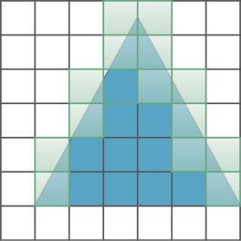
Figure 36.21: The triangle has binary visibility 1 on the pixels marked with solid blue and 0 on the pixels that are white. A binary value cannot accurately represent the triangle’s visibility on the pixels along the triangle’s slanted sides that are marked in light green. Attempting to compute binary visibility at those pixels necessarily produces aliasing.
The A-buffer [Car84] separates the coverage computation from the shading computation to address the overshading problem of SSAA. An A-buffer renderer computes coverage at each sample for a fragment. If at least one sample is covered, it appends the fragment to a list of fragments within that pixel. If that fragment completely occludes some fragment that was previously in the list, the occluded fragment is removed. When all primitives have been rasterized, shading proceeds on the fragments that remain within each pixel. The renderer computes a single shade per fragment and applies it to the covered and unoccluded samples within the pixel. This allows more accurate measurement of coverage due to geometric variation than shading. Because coverage is a simple and fixed computation, it can be computed far more efficiently than shading in general, and MSAA (covered shortly) enjoys the advantage that there is minimal overhead in increasing the number of samples per pixel. Thus, N samples may cost nearly the same as 1 sample.
The A-buffer can also be used to composite translucent fragments in back-to-front order. In this case, a fragment is not considered occluded if the occluding fragment is translucent. Fragments are sorted before shading and compositing. The drawback of the A-buffer is that the implementation requires variable space and significant logic within the coverage and rasterization process for updating the state. As a result, it is commonly used for offline software rendering. However, variations on the A-buffer that bound the storage space have recently been demonstrated to yield sufficiently good results for production use [MB07, SML11, You10]. These simply replace existing values when the maximum per-pixel sample list length is exceeded. A more sophisticated approach is to store some higher-order curve within a pixel that approximates all coverage and depth samples that have been observed. This approach has predominantly been applied to volumes of relatively homogeneous, translucent material, like smoke and hair [LV00, JB10].
Multisample antialiasing (MSAA) is similar to the A-buffer, but it applies a depth test and shades immediately after per-sample coverage computation to avoid managing per-pixel lists. This limits its application to spatial antialiasing, although stochastic approaches can extend temporal (motion blur), translucent, and lens (depth-of-field) sampling into the spatial domain [MESL10, ESSL10].
For each fragment, MSAA computes a coverage mask representing the binary visibility at each sample. In the most common application this is done by rasterizing and applying a depth buffer test with more samples than color pixels. If any sample was visible, an MSAA renderer then computes a single shading value for the entire pixel. The location of this shading sample varies between implementations; some choose the sample closest to the center of the pixel (regardless of whether it was visible!), and others choose the first visible sample. This single shading value is then used to approximate the shading at every sample in the pixel.
MSAA has several drawbacks. The first is that the shading computation must estimate the average value of the shade across the pixel rather than at a single point. In other words, MSAA leaves the problem of aliasing due to variation in the shading function to the shader programmer—it only reduces aliasing due to geometric edges. For a shader that computes the color of a flat, matte surface with uniform appearance, this is a good approximation. In contrast, a shader that samples specular reflections off of a bumpy surface may exhibit significant under-sampling because the shading function rapidly varies in space.
The second problem is that MSAA requires storage for a separate shade at each pixel. Thus, it has the same memory bandwidth and space cost as SSAA, even though it often reduces computation substantially.
Third, MSAA works best for primitives that are substantially larger than a pixel, and for pixels with many samples. If a mesh is tessellated so that each primitive covers only a small number of samples, then many shading computations are still needed.
Fourth and finally, MSAA does not work with the shading step of deferred shading algorithms. Deferred shading separates visible surface determination from shading. It operates in two passes. The first pass computes the inputs to the shading function at each sample and stores them in a buffer. The second pass iterates over each sample, reads the input values, and computes a shading value for the sample. When there are more samples than pixels, a final “resolve” operation is needed to filter and downsample the results to screen resolution. MSAA depends on amortizing a single shading computation over multiple samples. Under forward shading, that is possible because the coverage information for a single fragment is in memory at the same time that shading is being computed. Because deferred shading resolves coverage for all fragments before any shading occurs, the information about which samples within a pixel corresponded to the same fragment has been lost at shading time. Thus, one is faced with the two undesirable options of rediscovering which samples can share a shading result or of shading all samples by brute force.
Shading caches and decoupled shading [SaLY+08, RKLC+11, LD12] are methods currently under active research for adding a layer of indirection to capture the relationship between shading and coverage samples under a bounded memory footprint. The goal of this line of research is to combine the advantages of MSAA and deferred shading without necessarily creating an algorithmic framework that resembles either.
Coverage sampling antialiasing (CSAA) [You06] combines the strengths of the A-buffer and MSAA. It separates the resolution of coverage from both the resolution of shading and the resolution of the depth buffer. The key idea is that within each pixel there is a large set of high-resolution samples, but those samples are pointers to a small set of unique color (and depth, and stencil, etc.) values rather than explicit color values. For example, Figure 36.22 shows 16 sample locations within a pixel that reference into a table of four potentially unique color values.
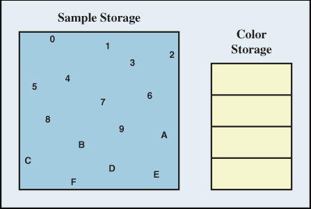
Figure 36.22: Depiction of the storage allocated for a single pixel under 16x CSAA [You06]. The large box on the left depicts the coverage samples. Each color sample contains a 2-bit integer that indexes into the four slots in the color table depicted by the smaller box on the right. When a fifth unique color is required, one of the four color samples is replaced. Thus, CSAA is heuristic and cannot guarantee correctness when many different surfaces color a pixel. (Courtesy of NVIDIA)
CSAA allows a more accurate estimate of the area of the fragment within the pixel than the estimate of the occlusion of a fragment by other fragments. As each fragment is rasterized, CSAA computes a single shade per pixel, many binary visibility samples ignoring occlusion, and a few binary visibility samples taking occlusion into account. A small, fixed number of slots (usually four) are maintained within each pixel that are similar to entries in an A-buffer’s list. Each slot stores the high-resolution coverage mask, shade value, and depth (and stencil) sample for a single fragment. Fragments are retained while there are some high-resolution coverage samples unique to them, and while there are available slots. When all of the slots are filled, some fragments are replaced. Thus, a pixel with 16 coverage samples and four slots may be forced to drop up to 12 fragments that actually should affect the pixel value. However, for primitives of screen-space area greater than one pixel it is often the case that only a few fragments will have nonzero coverage at a pixel. So, although CSAA is lossy, it often succeeds at representing fine-grained coverage using less storage than MSAA and the A-buffer, and with a low shading rate.
Analytic coverage historically predates CSAA, but can be thought of today as the limit of the CSAA process. Rather than taking many discrete samples of fragment coverage ignoring occlusion, one might simply compute the true coverage of a pixel by a fragment from the underlying geometric intersection. In the case of an instantaneous pinhole camera and simple surface geometry, this is a straightforward measure of the area of a convex polygon. The ratio of that area to the area of the pixel is the partial coverage of the pixel by that surface.
In the context of rasterization, for some primitives this computation can be amortized over many pixels so that computing analytic partial coverage information adds little cost to the rasterization itself. Primitives for which efficient partial coverage rasterization algorithms are known include lines [Wu91, CD05a] and circles [Wu91], which naturally extend to polygons and disks by neglecting one side.
Modern hardware rasterization APIs such as OpenGL and Direct3D include options to compute partial coverage for these primitives as part of the rasterization process. The implementation details vary. Sometimes the underlying process involves taking a large number of discrete samples rather than computing the true analytic result. Since there is a fixed precision for the result, the difference is irrelevant once enough samples are taken.
Analytic coverage has the advantage of potentially significantly higher precision than multiple discrete samples, with no additional memory or shading cost per pixel. It is often used for rasterization of thin lines and for polygons and curves in 2.5D presentation graphics and user interfaces.
The tremendous drawback of analytic coverage is that by computing a single partial-coverage value per fragment, it loses the information about which part of the pixel was covered. Thus, the coverage for two separate fragments within the pixel cannot be accurately combined. This problem is compounded when occlusion between fragments is considered, because that alters the net coverage mask of each. Porter and Duff’s seminal paper [PD84] on this topic enumerates the ways that coverage can combine and explains the problem in depth (see Chapter 17). In practice, their OVER operator is commonly employed to combine fragment colors within a pixel under analytic antialiasing. In this case, there is a single depth sample per pixel, a single shade, and continuous estimation of coverage. Let α represent the partial coverage of a new fragment, s be its shading value, and d be the shading value previously stored at the pixel. If the new fragment’s depth indicates that it is closer to the viewer than the fragment that previously shaded the pixel, then the stored shade is overwritten by αs + (1 – α)d. This result produces correct shading on average, provided that two conditions are met. First, fragments with α < 1 must be rendered in farthest-to-nearest order so that the shade at a pixel can be updated without knowledge of the fragments that previously contributed to it. Second, all of the fragments with nonunit coverage that contribute to a pixel must have uncorrelated coverage areas. If this does not hold, then it may be the case, for example, that some new fragment with α = 0. 1 entirely occludes a previous fragment with the same coverage, so the shade of the new one should overwrite the contribution of the former one, not combine with it.
In the case of 2.5D presentation graphics, it is easy to ensure the back-to-front ordering. The uncorrelated property is hard to ensure. When it is violated, the pixels at the edges between adjacent primitives in the same layer are miscolored. This can also occur at edges between primitives in different layers, although the effect is frequently less noticeable in that case.
Give an example, using specific coverage values and geometry, of a case where the monochrome shades from two fragments combine incorrectly at a pixel under analytic occlusion despite correct ordering.
36.9.2. Defocus (uv)
For a lens camera, there are many transport paths to each point on the image plane. The last segment of each path is between a point on the aperture and a point on the image plane. The “rays” between points on the image plane and points in the scene are not simple geometric rays, since they refract at the lens. However, we only need to model visibility between the aperture and the scene, since we know that there are no occluders inside the camera body.
For a scene point P there is a pencil of rays that radiate toward the aperture. For example, if the aperture is shaped like a disk, these rays lie within a cone. We can apply the binary visibility function to the rays within the pencil.
If there are no occluding objects in the scene and the camera is focused on that point, the lens refracts all of these rays to a single point on the image plane (assuming no chromatic aberration; see Chapter 26). The point Q on the image plane to which P projects in a corresponding pinhole camera thus receives full coverage from the light transported along the original pencil of rays.
If the point is still in focus, but an occluder lies between the scene point and the lens in such a way that it blocks only some of the rays in the pencil from reaching the aperture, then only some of the light leaving the point toward the aperture will actually form an image. In this case, depicted in Figure 36.23, Q only receives partial coverage from P.
If there are no occluders but P is out of focus, then the light from the pencil originating at P is spread over a region on the image plane. Point Q now receives only a fraction of the light that it did in the in-focus case, so it now receives partial coverage by P.
Of course, a point may have partial coverage because it is both out of focus and partly occluded, and other sources of partial coverage can combine with these as well.
Note that in a sense any point is partially occluded by the camera case and finite lens—there are light rays from a scene point that would have struck the aperture had the lens only been larger. For a lens camera it is always necessary to know the size of the lens to compute the total incident light. The total light is proportional to the partial coverage, but we must know the size of the lens to compute the total power.
One way to compute partial coverage due to defocus is to sample visibility at many rays within the pencil and average the result. Because all the rays of the pencil share a common origin, there is an opportunity to amortize the cost of these binary visibility operations. The packet tracing and rasterization algorithms discussed in Chapter 15 leverage this observation.
36.9.3. Motion Blur (t)
Just as real cameras have nonzero aperture areas, they also have nonzero exposure times. This means that visibility can vary throughout the exposure. For any specific time, binary visibility may be determined between two points. The net visibility during an exposure will be the integral of that binary visibility over the exposure period, during which primitives may potentially cross between the points, producing an effect known as motion blur. For primary visibility in the presence of motion blur, we must consider the fact that the points for which we are testing visibility are on curves through space and time. This is easily resolved by performing all tests in camera space, where the primary rays are static with respect to time. Then we need only consider the motion of the scene relative to the camera.
Spatial data structures must be extended to represent motion. In particular, a spatial structure needs to bound the extrusion of each primitive along its motion path during the exposure. This step was not necessary for defocus because in that case we were performing ray-intersection queries that varied only the rays, not the triangles. When the triangles move with respect to each other a data structure built for a single position is no longer valid. A common strategy is to first replace each primitive with a conservative (and typically convex) bound on its motion. The second step is then to build the hierarchy on those proxies rather than the primitives themselves. When thin primitives rotate this can create excessively conservative bounds, but on the other hand, this approach is relatively straightforward to implement compared to considering the complex shapes that tightly bound rotating primitives.
This strategy generalizes to simply considering ray casting as a “four-dimensional” problem, where both rays and surfaces exist in a 4D space [Gla88]. The first three dimensions happen to be spatial and the fourth is temporal, but mathematically one can frame both the ray-intersection problem and the spatial data structure construction so that they are oblivious to this distinction. For a bounding box hierarchy, the result is the same as was described in the previous paragraph. However, with this generality we can consider arbitrary bounding structures, such as a 4D BSP tree or bounding sphere hierarchy, which may provide tighter (if less intuitive) bounds.
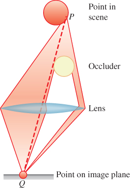
Figure 36.23: Partial occlusion of the lens leads to partial occlusion of the single point P at point Q.
36.9.4. Coverage as a Material Property (α)
A single geometric primitive may be used as a proxy for more complex geometry, for example, representing a window screen or a maple leaf as single rectangle. In this case, the small-scale coverage can be stored as a material property. By convention this property is represented by the variable α. Alpha is explicit coverage: α = 0 is no coverage (e.g., areas outside of the leaf’s silhouette), α = 1 is total coverage (e.g., areas inside the leaf’s silhouette), and 0 < α < 1 is partial coverage (e.g., the entire window screen may be represented with α = 0. 5).
Under what circumstances (e.g., position of the object relative to other objects or the camera) might the use of coverage-as-material-property lead to substantial errors in an image?
Note that a single α value is insufficient to represent colored translucency. A red wall viewed through a green wine bottle should appear black. Yet, if we model a bottle with a green surface as α = 0. 5, we will observe a brown wall through the bottle, whose color is 50% red and 50% green. This is a common artifact in real-time rendering. Offline rendering tends to model this situation more accurately with one coverage value per frequency of light simulated, or by sampling the light passing through the bottle as scattered rather than composited. This can also be done efficiently for real-time rendering by trading spatial precision for coverage precision [ME11].
An explicit coverage α must still be injected into the coverage resolution scheme for the entire framebuffer. Two common approaches are analytic and stochastic coverage. For the analytic approach, one simply renders in back-to-front order (with all of the limitations this implies) and explicitly composites each fragment as it is rendered, or injects the fragments into an A-buffer for it to process in that manner during resolution.
Stochastic approaches randomly set the fraction of coverage mask bits approximately equal to α and then allow another scheme such as MSAA to drive the shading and resolve operations. It is essential to ensure that the choice of which coverage bits are set is statistically independent for each fragment [ESSL10] because this is an underlying assumption of the compositing operations [PD84] implicit in the resolve filter.
Recent work shows that the quality of the resolve operation for stochastic antialiasing methods can be improved by filters more sophisticated than the typical box filter, although it has yet to be shown that the cost of complex resolve operations is less than the cost of simply increasing the number of samples [SAC+11].
36.10. Discussion and Further Reading
The classic paper “A characterization of ten hidden-surface algorithms” by Sutherland and Sproul [SSS74] surveys the state of the art for visibility in 1974, when the typical goal was to determine the set triangles visible to the camera. None of those algorithms are in common use today for primary visibility on triangles. They’ve been replaced by the brute force z-buffer and by coarse hierarchical occlusion culling. However, it is worth familiarizing yourself with the algorithms Sutherland and Sproul surveyed for other potential applications. For example, we saw that BSP trees [SBGS69, FKN80] were originally designed to order polygons by depth so that they could be rendered perfectly using a variant of the painter’s algorithm. BSP trees became popular for computing polygon-level visibility in game rendering engines in the 1990s and they are at the heart of a popular illumination algorithm [Jen01] used on most CG film effects today. Instead of ordering polygons for back-to-front rendering, BSP trees were found to be an effective way of carving up 3D space for O(log n) access to surfaces and creating convex cells between which visibility determination is efficient. We anticipate that today’s visible surface algorithms and data structures will find similar new uses in another 30 years, while newer and better approaches to visibility determination evolve as well.
36.11. Exercise
Exercise 36.1: Typically in Sutherland-Hodgman clipping, the polygon to be clipped is small compared to the boundary polygon, and it intersects at most one side of the boundary polygon; often the input polygon starts on the inside, crosses the boundary, remains outside for a while, and then recrosses the same boundary edge and returns inside. In this case, clipping an input polygon with n edges against a boundary with k edges involves generating and inserting only two intersection points, although it involves testing O(nk) edge pairs for intersections. Build an example input in which there are O(nk) intersection points computed and inserted.