Chapter 23. Splines and Subdivision Surfaces

23.1. Introduction

Both spline curves and subdivision curves can be generalized, creating spline and subdivision surfaces. In this chapter, we show how to make a Bézier patch: a small piece of surface, parameterized by [0, 1] × [0, 1], for which u S(u, v₀) is a Bézier curve for each value of v₀ and v S(u₀, v) is a Bézier curve for each value of u₀ (i.e., “it’s Bézier in both directions”). Just as Bézier curves can be joined together into longer curves, Bézier patches can be assembled together into a “quilted” surface, although making the patches meet up smoothly at the edges and corners is more complex than in the curve case. The quilt, in this situation, generally has the form of a grid: squares meeting four at a corner. The web material for this chapter describes the creation of spline surfaces in more detail.

If we want to make a shape where adjacent patches meet three at a corner or five at a corner, the conditions for continuity are much messier and the resultant shape is not as controllable. One popular solution in this case is to shift to subdivision surfaces, which start from an arbitrary polyhedron and, through repeated subdivision, converge to a surface that’s generally very smooth. In the subdivision scheme we present in this chapter we can start from any polygonal mesh, but after subdivision all faces of the mesh become quadrilateral, and after repeated subdivision most vertices meet exactly four faces. Faces whose vertices all have valence four can be shown to be the same as cubic spline surfaces, which meet their neighbors with C² smoothness. At the “exceptional” vertices, where three or five or six or more faces meet, the surface is generally C¹ smooth, but it may have curvature discontinuities. The web material for this chapter describes various further subdivision schemes and their implementation.

23.2. Bézier Patches

Just as a Bézier curve was defined by a sequence of four points P₁, P₂, P₃, and P₄, we’ll describe a Bézier patch by a mesh of 16 points, P_ij, where i and j range from 1 to 4. Writing

for the ith Bézier basis function, the Bézier curve based on P₁₁, P₁₂, P₁₃, and P₁₄ is

There’s nothing special about the “1” in this formula—a Bézier curve can be constructed based on any row of points in the mesh. The same goes for the columns. If we combine the two, we can build a parameterized surface:

The function S is defined for 0 ≤ u, v ≤ 1. If we hold v fixed—say, at v = 0—we get

Since b_j(0) = 0 for j = 2, 3, 4, and b₁(0) = 1, this simplifies to

so S(u, 0) traverses a Bézier curve as u varies from 0 to 1, with control points P_i1, i = 1, 2, 3, 4. Similarly, S(u, 1) traverses a Bézier curve with control points P_i4, and S(0, v) and S(1, v) traverse Bézier curves with control points along the other two edges of the mesh.

In fact, for any fixed value of v—say, v₀—S(u, v₀) traverses a Bézier curve: The surface defined by S is made up of a family of Bézier curves, one for each value of v₀, as Figure 23.1 shows. But the same is true in the other direction: As we hold u fixed and vary v, we also get a Bézier curve.

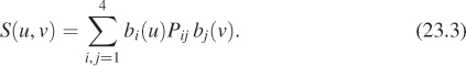
Figure 23.1: (Top) A Bézier patch drawn with the collection of curves t S(s, t) for several values of s between 0 and 1. (Middle) The same patch, drawn with the curves s S(s, t) for several values of t. (Bottom) The same surface, drawn colored by height. In the top two drawings, the control mesh Q_ij(0 ≤ i, j ≤ 3) is shown.

The shape of the surface patch we’ve just described is controlled by the locations of the control points P_ij. The surface passes through the four corner points P₁₁, P₁₄, P₄₄, and P₄₁. The points on the interior of each edge, like P₂₁ and P₃₁, control the shapes of the edges of the patch. For instance, the tangent plane to the patch at P₁₁ contains both the vector P₂₁ – P₁₁ and the vector P₁₂ – P₁₁, so the cross product of these two vectors is the surface normal at P₁₁. The four interior control points determine the shape of the center region of the patch without influencing the patch boundary. They do, however, affect the direction in which the patch meets its boundary. If you plan to work with patches like this, you should write a small interactive application in which you can manipulate each control point to see its effect on the surface shape.

The surface we’ve just described is called a bicubic tensor product patch, because it’s made by using products of basis functions, each of which is a cubic. If, in the expression b_i(u)P_ijb_j(v) of Equation 23.3, we replaced b_i(u) with c_i(u), where c_i is the ith basis function for the Hermite curve, or the ith Catmull-Rom basis, or the ith cubic B-spline basis, we’d get different kinds of tensor product patches: The effects of the control points on the eventual shape would depend on the kinds of basis functions used. You could make a patch that used Bézier curves in one direction and Hermite in the other, for instance.

Just as we glued together curve segments to get longer curves, we can do similar things to get larger surfaces. We can try to place two surface patches next to each other so that they match up along a single edge. In the case of the Bézier-based patches described above, the rightmost column of control points for one patch must match the leftmost column of control points for the other, for instance. This will guarantee that the surfaces join up (their joining edges consist of a single Bézier curve), but not that they join up smoothly. For a smooth join, without a crease along the joining curve, further conditions on the adjacent two columns of control points are needed.

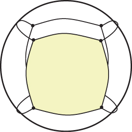
Arranging a gridlike “quilt” of patches requires that a substantial collection of constraints be met; the web material for this chapter describes some of these. But when we try to make rectangular patches glue together in a pattern that has them meet three at a vertex, as in Figure 23.2, the constraints become overwhelming. There are several solutions: We can deal with the overwhelming constraints and continue to use rectangular patches, or we can shift to something like triangular patches, where gluing together is a little easier, or we can, as we did with curves, move to subdivision as a way to create shapes. We’ll now briefly discuss this third approach.

Figure 23.2: A spherical blob made from six “rectangular” patches that meet three at a vertex.

23.3. Catmull-Clark Subdivision Surfaces

Subdivision surfaces don’t start with individual patches to be joined: They start from a polygonal mesh, which is repeatedly modified to approach a usually smooth limit surface. This simplifies matters a good deal.

In the Catmull-Clark subdivision scheme [CC98, HKD93], we start with a mesh, typically in R³ (although the process works in any dimension). The vertices of each face need not actually be coplanar, although it’s easiest to visualize the subdivision process if they’re nearly coplanar, so we’ll start with an example where this is true (see Figure 23.3). The faces of the initial mesh may be triangles, quads, pentagons, etc., but after one level of subdivision all faces will be quads, so we’ve drawn an example where they are all quads.

Figure 23.3: A mesh where one vertex v has n adjacent vertices e₁, e₂, . . . e_n, at the ends of the edges, leaving v.

Just as with subdivision curves, we’ll describe subdivision surfaces in terms of a neighborhood of a vertex v, that is, a set of vertices near v in the graph structure of the mesh.

The first step of subdivision is to compute the centroid (the average of the vertices of the ith face). (We’ll follow the convention that primes denote points of the subdivided mesh, and unprimed symbols denote points of the mesh before subdivision.)

We next compute the edge points by the formula

All subscripts are taken modulo n.

Finally, we compute a new location for the vertex v:

These new locations are connected as shown in Figure 23.4.

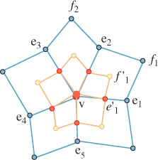
Figure 23.4: The new vertex is connected to each new edge point; the new edge points are connected to the face points for adjacent faces (illustrated for case n = 5).

After subdivision, there are approximately four times as many faces as before subdivision. After just a few levels of subdivision, we’ll have a great many faces.

The special case n = 4 (which is the most common, as shown by the preceding exercise) is worth examining.

In this case, Equation 23.7 becomes

which says that v′ is a weighted average of v, the average of the adjacent edge points, and the average of the adjacent face points, just as for curve subdivision the new vertex location was an average of the old vertex location and the average of the adjacent edge points.

This situation (after the first level of subdivision) is shown in Figure 23.5.

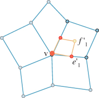
Figure 23.5: For a quad mesh, the face vertices from the previous level of subdivision are opposite v in each quad.

In this case, we can rewrite the subdivision formula for v′ in terms of v, {e_i}, and {f_i} instead of using {}; all we need to do is substitute

to get

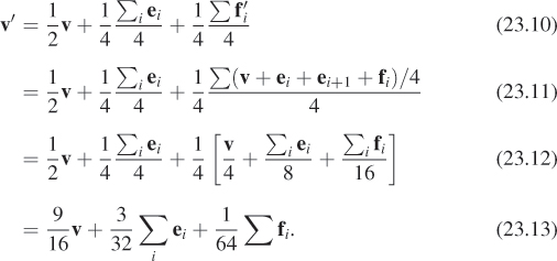
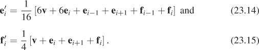
Corresponding formulas for and in terms of the pre-subdivision vertices are

If we list the coordinates of the central vertex v, then the edge vertices e₁, e₂, e₃, e₄, and then the face vertices f₁, ..., f₄ in a 9 × 3 matrix, V, we can summarize by saying that

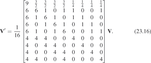
More generally, for a vertex of degree n, there are 2n + 1 rows in V and the subdivision matrix is a (2n + 1) × (2n + 1) matrix. Letting V_n denote the neighborhood coordinates for a vertex of degree n, we can write

where the matrix S_n is of the appropriate size. Everything about Catmull-Clark subdivision can be determined by studying the matrix S. Halstead et al. [HKD93] carry this out in some detail.

As an example of what one can derive, if we look at some vertex v in a mesh, during repeated subdivision v will approach some point v^∞. (This can be proved by looking at powers of S; the web materials for this chapter do so explicitly.) The limit point point v^∞ for v under repeated subdivision is

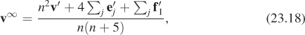
where the primes indicate one level of subdivision. (This is determined by looking at eigenvectors of S.) Notice that v need not be a vertex of the original mesh. If, after three levels of subdivision, we insert a new face point, we can call this point v, find its neighboring face and edge points, and apply the limit formula above.

We can now make three observations.

First, the formula for computing the limit point does exactly the same computation with the x-, y-, and z-coordinates. In fact, it works in any dimension at all, and we can think about subdivision surfaces one coordinate at a time.

Second, if the initial mesh consists of the integer lattice in the xy-plane (i.e., all integer points are vertices, and the unit-length vertical and horizontal segments joining them are the edges), then a single subdivision operation produces the half-integer lattice, two subdivisions produce the quarter-integer lattice etc.

Third, if we alter the integer lattice by replacing (0, 0, 0) with (0, 0, 1), the limit surface shown in Figure 23.6 is very simple. In fact, just as for subdivision curves, it turns out that this limit surface is actually identical to the cubic B-spline basis function. In particular, if (x, y, z) is on the limit surface, then B(x, y) = z, where B is the basis function.

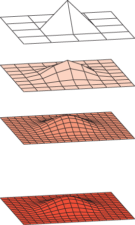
Figure 23.6: (Top) The initial mesh consists of the integer lattice with one point raised. (Middle) The first and second levels of subdivision. (Bottom) The cubic B-spline basis function whose control points are the vertices of the original control mesh, for comparison.

This means that, at least in areas where the mesh has standard lattice connectivity, the limit subdivision surface is the same as the B-spline surface defined by those control points. Since code for computing and rendering such surfaces is widely available, this is very convenient. In any neighborhood of an exceptional vertex (i.e., one whose degree is different from four), the limit surface is not similar to a B-spline, and we have to compute the surface by repeated subdivision. Stam [Sta98] discusses the limit shape both at and away from exceptional points.

Analysis like that for the limit points also shows how to compute the normal vector at the limit point [HKD93], at least for vertices in sufficiently general position. (There are configurations for which the limit surface does not have a well-defined normal, just as there are B-spline curves that have geometric cusps, despite being parametrically smooth.)

Since both the limiting position and the surface normal are expressible as linear combinations of a few neighboring vertices, one can solve problems like “Find me initial vertex positions for this mesh with the property that the limit surface passes through these points and has these normal vectors at them.” This is the central problem addressed by Halstead et al.

While the limit surface for subdivision is generally smooth, at exceptional vertices it may not be curvature-continuous (i.e., the curvature at the limit of an exceptional vertex may be undefined, or it may not be continuous in a neighborhood of that vertex). One might try to address the surface to be curvature-continuous through a kind of “surgery”: Remove a small disk around the offending point and replace it with a smooth surface. But guaranteeing continuity at the seam is problematic. As an alternative, one can blend between the limit surface and a smooth replacement, using a blending function that’s a sufficiently smooth function of the distance from the exceptional point and that varies from 0 at the seam to 1 at the center, with all derivatives being 0 both at the seam and at the center. Such an ad hoc approach requires choosing a radius for the disk and choosing a smooth shape to blend with, but it can be made to work quite well in practice [Lev06]. A different approach, based on improving the appearance of the exceptional point rather than its geometry, is to use the “approximate Catmull-Clark subdivision surfaces,” or ACC surfaces, developed by Loop and Schaeffer [LS08]. Starting from the mesh to be subdivided, they develop, for every quad, a bicubic patch (u, v) S(u, v) that represents the geometry of the limit surface, and two associated patches t_u(u, v) and t_v(u, v) where the value of t_u(u, v) approximates the tangent vector to S in the u direction at (u, v), that is, , and similarly for t_v. These approximate tangent-vector functions can be used to compute an approximate normal that varies smoothly over the surface, that is, that gives the limit surface the appearance of smoothness when this approximate normal vector is used in rendering it.

23.4. Modeling with Subdivision Surfaces

We’ve indicated, in our discussion of Catmull-Clark surfaces, how subdivision surfaces can be fitted to point and normal data. But when you have a shape in mind and want to create a model, point and normal data is not available. One approach is to make a physical model of your shape, scan it, and then fit a surface to it; this approach is used by many production studios. But as an alternative, one can model directly with subdivision surfaces.

A typical modeling session starts with a coarse mesh that the user adapts to have the general shape of the object of interest. The user then subdivides this mesh and adjusts the locations of some of the resultant vertices. Often the subdivision process puts the new mesh just about where the user expects, and new vertices need adjustment only to add detail. After another level of subdivision, the user adds more detail, etc. At some point, the surface shape is satisfactory and the limit surface is computed (or perhaps a few more stages of subdivision are performed to generate an effectively smooth mesh).

Adjusting vertex positions after a level of subdivision is acceptable because the resultant mesh is an acceptable input to the subdivision algorithm. Indeed, one can go further: One can actually edit the topology of a mesh, adding a hole at some level, etc. The data that needs to be recorded for such a modeling session consists of the original vertex positions, plus any edits made at each level. In the event that several vertices at level three, say, were all moved in the same direction, there may be a level-two edit that would have achieved the same effect, or most of it. Rewriting the representation to include this level-two edit, and then smaller level-three edits, may make the representation more compact.

This editing approach has the advantage that the user can “browse” through different levels, adjusting the shape at higher levels and then returning to lower levels. One problem that arises is that details added at a lower level may not make sense after a high-level edit. In a face model, for instance, a nose might be drawn out in the x-direction. If at a higher level, the face is rotated by 90° in the xy-plane, the low-level edit will make a nose that’s dragged to the side of the face rather than in front of it. It therefore is useful to express low-level edits in a coordinate system that’s tied to the result of higher-level subdivision so that the nose is described as being drawn out along the normal to the face, rather than “in the x-direction.” Such multiscale editing is described by Cohen et al. [MCCH99], and the condensation of multiscale editing representations, together with other multiscale editing techniques, is described by Zorin et al. [ZSS97].

23.5. Discussion and Further Reading

As with the preceding chapter, the web material for this chapter contains a much-expanded version of the material presented here, together with pointers to the literature. Spline and subdivision surfaces are at the heart of most of today’s CAD packages, and CAD long ago became its own area, largely separate from computer graphics. Introductory CAD texts will help you grasp the main ideas (and some of the sometimes-complex indexing schemes!). Loop’s Master’s thesis [Loo87] is a gentle introduction. Despite the separation of graphics and CAD, there continues to be cross-fertilization.