Chapter 10. Convective Mass Transfer: Theory for Internal Laminar Flow

Search in book...
Toggle Font Controls
Create new playlist

Name your new playlist

Playlist description (optional)
Sign In

Email address

Password

Forgot Password?

or

Continue with Facebook

Continue with Google
Sign Up

Full Name

Email address

Confirm Email Address

Password

or

Continue with Facebook

Continue with Google

Chapter 10. Convective Mass Transfer: Theory for Internal Laminar Flow

Learning Objectives

After completing this chapter, you will be able to:

Formulate models for mass transfer under laminar flow in confined geometries.
Express the model in dimensionless form and identify dimensionless groups.
Solve for mass transfer in fully developed flow from a pipe using the hypergeometric function.
Model and solve for mass transfer in the entry region of a pipe using the similarity solution method.
Solve for convective mass transfer with wall reaction using the CHEBFUN code.
Model mass transfer rate in solid dissolution and gas absorption from a falling film.
Use the PDEPE solver for numerical solution of convective mass transfer problems in a more general setting.

Convective mass transfer problems are best studied in two categories of flow: internal flows in confined geometries where flow becomes fully developed and external flows, which are essentially of the boundary layer type. This chapter deals with problems with internal flows, for example, flow in a pipe, flow in a square channel, and similar situations, while the next chapter deals with problems where a boundary layer type of analysis is needed.

The first problem studied in this chapter is that of mass transfer in pipe flows. The velocity profile is assumed to be fully developed and a parabolic function for Newtonian fluids. Using this profile, the convection diffusion equation is solved. The concentration is now a function of two coordinate directions, namely the axial distance and the radial (or cross-flow) direction and therefore the governing equations are now partial differential equations (PDEs). Mathematically speaking the PDEs are similar to that for transient mass transfer studied in an earlier chapter; hence the method of separation of variables can be used. But in the context of convective transport these PDEs, although still linear, have variable (position dependent) coefficients. This adds additional mathematical complexity to the solution, mainly in the form of the eigenfunctions and the calculations of the eigenvalues. These details will be examined. Nature of the series, convergence properties, mass flux, and the predicted mass transfer coefficients will be examined and illustrative examples are presented. The methodology is the same for channel flows and duct flows and we show some illustrative results for this case as well.

An alternative method using the similarity variable is more useful in the entry region to a pipe. The boundary layer nature of the concentration distribution near the entrance region permits this approach. We will define the similarity variable and derive a closed form analytical solution to the entry region problem for pipe flow.

The next class of problems studied is those in convective mass transfer in film flows. The mass transfer into a liquid flowing as film over a vertical (or inclined) surface is an important prototype problem in convective mass transfer since it simulates the flow in more complex industrial equipment such as packed beds. We examine two important cases here: solid dissolving from the wall and gas being absorbed from the interface of the liquid film. We explore the similarity solution approach to predict the mass transfer coefficients for the two cases. We will also compare and contrast the two problems.

The final section of the chapter deals with numerical solution of convective transport problems. Mainly the use of the PDEPE solver in MATLAB and CHEBFUN is demonstrated. Some analytical results will be used to benchmark the numerical results. Next numerical results for some additional problems will be presented.

10.1 Mass Transfer in Laminar Flow in a Pipe

The starting point is the convection-diffusion equation introduced in Chapter 5:

\begin{matrix} υ \cdot \nabla C_{A} = D_{A} \nabla^{2} C_{A} & (10.1) \end{matrix}

$\begin{matrix} υ \cdot \nabla C_{A} = D_{A} \nabla^{2} C_{A} & (10.1) \end{matrix}$

In this section we apply this to solve mass transfer in a fully developed flow in a circular pipe. In such cases the velocity has only the z-component and the velocity profile (for a Newtonian fluid) is given as

υ_{z} = 2 〈 υ 〉 [1 - (\frac{r}{R})^{2}]

$υ_{z} = 2 〈 υ 〉 [1 - (\frac{r}{R})^{2}]$

Here 〈v〉 is the average velocity. The Laplacian term is used with the r- and z-directions as there is no variation of the concentration in the θ direction. The governing equation is therefore

\begin{matrix} 2 〈 υ 〉 [1 - (\frac{r}{R})^{2}] \frac{\partial C_{A}}{\partial z} = D_{A} [\frac{\partial^{2} C_{A}}{\partial z^{2}} + \frac{1}{r} \frac{\partial}{\partial r} (r \frac{\partial C_{A}}{\partial r})] & (10.2) \end{matrix}

$\begin{matrix} 2 〈 υ 〉 [1 - (\frac{r}{R})^{2}] \frac{\partial C_{A}}{\partial z} = D_{A} [\frac{\partial^{2} C_{A}}{\partial z^{2}} + \frac{1}{r} \frac{\partial}{\partial r} (r \frac{\partial C_{A}}{\partial r})] & (10.2) \end{matrix}$

The solution to this problem is now studied with suitable boundary conditions at the walls. Before proceeding further, a note on the entry region for flow is in order. In this formulation (10.2), we assume that z = 0 is at a location in the pipe where the velocity profile is already fully established. This requires a hydrodynamic entry length, L_e, given by the following equation:

\frac{L_{e}}{R} = 0.0 7 R e

$\frac{L_{e}}{R} = 0.0 7 R e$

Hence z = 0 is not the actual entrance of the flow and represents a starting point after the hydrodynamic entry region. We assume mass transfer conditions start beyond this point. If the mass transfer starts at a position earlier than this length $L_{e}^{*}$ $L_{e}^{*}$ , the Equation 10.2 has to be modified since the velocity profile is not unidirectional in the entry region for flow. Flow is of the boundary layer type here and both υ_z and υ_r contribute to convective transport for that case.

10.1.1 Dimensionless Form

In dimensionless form the following equation can be derived:

\begin{matrix} (1 - ξ^{2}) \frac{\partial c A}{\partial z *} = \frac{1}{P e} [\frac{\partial^{2} c A}{\partial z *^{2}} + \frac{1}{ξ} \frac{\partial}{\partial ξ} (ξ \frac{\partial c A}{\partial ξ})] & (10.3) \end{matrix}

$\begin{matrix} (1 - ξ^{2}) \frac{\partial c A}{\partial z *} = \frac{1}{P e} [\frac{\partial^{2} c A}{\partial z *^{2}} + \frac{1}{ξ} \frac{\partial}{\partial ξ} (ξ \frac{\partial c A}{\partial ξ})] & (10.3) \end{matrix}$

Here z* is the dimensionless axial distance defined as z/R and ξ is the dimensionless radial distance defined as r/R. Also, c_A is a suitably defined dimensionless concentration.

Hence the parametric representation of the problem is

c_A = c_A(z*, ξ; Pe)

The parameter Pe appearing in dimensionless form (Equation 10.3) is defined as follows:

P e = \frac{〈 υ 〉 d_{t}}{D_{A}} = \frac{〈 υ 〉 d_{t}}{ν} \frac{ν}{D_{A}} = R e S c

$P e = \frac{〈 υ 〉 d_{t}}{D_{A}} = \frac{〈 υ 〉 d_{t}}{ν} \frac{ν}{D_{A}} = R e S c$

where Re is the Reynolds number based on the pipe diameter d_t and Sc is the Schmidt number defined as ν/D_A.

This dimensionless group has the following significance:

P e = \frac{mass transport by convection}{mass transport by diffusion}

$P e = \frac{mass transport by convection}{mass transport by diffusion}$

This can also be realized by writing Pe as

P e = \frac{〈 υ 〉 d_{t}}{D_{A}} = \frac{< υ > Δ C_{A}}{D_{A} Δ C_{A} / d_{t}}

$P e = \frac{〈 υ 〉 d_{t}}{D_{A}} = \frac{< υ > Δ C_{A}}{D_{A} Δ C_{A} / d_{t}}$

where ΔC_A is some representative concentration difference in the system. The numerator is a measure of convective transport while the denominator is a measure of diffusive transport; therefore the Peclet number is the ratio of the two modes of transport.

Simplification for Large Peclet Number

If Pe > 10, the convection term will dominate over diffusion in the axial direction. Hence the following approximation can be made:

\frac{\partial^{2} c_{A}}{\partial z *^{2}} < < \frac{1}{ξ} \frac{\partial}{\partial ξ} (ξ \frac{\partial c A}{\partial ξ})

$\frac{\partial^{2} c_{A}}{\partial z *^{2}} < < \frac{1}{ξ} \frac{\partial}{\partial ξ} (ξ \frac{\partial c A}{\partial ξ})$

and the model can be reduced considerably. This can be illustrated by a detailed scaling analysis, which is not shown here. Hence for large Peclet numbers the axial diffusion can be dropped, resulting in

\begin{matrix} (1 - ξ^{2}) \frac{\partial c A}{\partial z *} = \frac{1}{P e} [\frac{1}{ξ} \frac{\partial}{\partial ξ} (ξ \frac{\partial c A}{\partial ξ})] & (10.4) \end{matrix}

$\begin{matrix} (1 - ξ^{2}) \frac{\partial c A}{\partial z *} = \frac{1}{P e} [\frac{1}{ξ} \frac{\partial}{\partial ξ} (ξ \frac{\partial c A}{\partial ξ})] & (10.4) \end{matrix}$

This suggests that a rescaling of the dimensionless axial distance may be useful. Let us define ζ (zeta) as

\begin{matrix} ζ = \frac{z *}{P e} & (10.5) \end{matrix}

$\begin{matrix} ζ = \frac{z *}{P e} & (10.5) \end{matrix}$

This is also called the contracted axial distance parameter.

Equation 10.4 reduces to

\begin{matrix} (1 - ξ^{2}) \frac{\partial c A}{\partial ζ} = \frac{1}{ξ} \frac{\partial}{\partial ξ} (ξ \frac{\partial c A}{\partial ξ}) & (10.6) \end{matrix}

$\begin{matrix} (1 - ξ^{2}) \frac{\partial c A}{\partial ζ} = \frac{1}{ξ} \frac{\partial}{\partial ξ} (ξ \frac{\partial c A}{\partial ξ}) & (10.6) \end{matrix}$

The parametric representation now simplifies to

c_A = c_A(ζ, ξ)

No free parameter appears, which is a characteristic of a well scaled problem.

The solution to the model for the case of constant wall concentration will now be examined.

This problem is also known as the Dirichlet problem for laminar convection or the Graetz problem for mass transfer. Note that the problem has an exact analogy to the problem of heat transfer with constant wall temperature. This was first studied by Graetz in 1883.

10.1.2 Constant Wall Concentration: The Dirichlet Problem

For the case of constant wall concentration, the dimensionless concentration is defined as

c_{A} = \frac{C_{A} - C_{A s}}{C_{A, i} - C_{A s}}

$c_{A} = \frac{C_{A} - C_{A s}}{C_{A, i} - C_{A s}}$

The dimensionless inlet concentration is now 1 while the wall concentration is zero with this definition. This is convenient to make the problem homogeneous. The symmetry condition is applied at ξ = 0 as usual. Hence the boundary conditions for a constant wall concentration case for Equation 10.6 are as follows:

Entrance, ζ = 0: c_A = 1
Wall, ξ = 1: c_A = 0
Center, ξ = 0: ∂c_A/∂ξ = 0

Note that only one condition in the axial direction ζ (entrance condition) is needed. This would not be the case if the axial diffusion term were to be retained in the model. Two boundary conditions are needed in the radial direction ξ.

The problem, being linear, can be solved by separation of variables. Mathematical details are skipped and the final series solution is shown here.

The solution can be represented as a series of the form

\begin{matrix} \begin{matrix} c_{A} (ζ, ξ) = \sum_{n = 1}^{\infty} C_{n} exp (- λ_{n}^{2} ζ) F_{n} (ξ) \end{matrix} & (10.7) \end{matrix}

$\begin{matrix} \begin{matrix} c_{A} (ζ, ξ) = \sum_{n = 1}^{\infty} C_{n} exp (- λ_{n}^{2} ζ) F_{n} (ξ) \end{matrix} & (10.7) \end{matrix}$

where λ_n are the eigenvalues to the associated eigenproblem and F_n are the eigenfunctions. The associated eigenvalue problem is the differential equation for F. This equation can be derived by substituting the proposed solution Equation 10.7 in Equation 10.6; you should verify that the following eigenvalue problem is obtained:

\begin{matrix} \frac{\partial}{\partial ξ} (ξ \frac{\partial F_{n}}{\partial ξ}) = - λ_{n}^{2} ξ (1 - ξ^{2}) F_{n} & (10.8) \end{matrix}

$\begin{matrix} \frac{\partial}{\partial ξ} (ξ \frac{\partial F_{n}}{\partial ξ}) = - λ_{n}^{2} ξ (1 - ξ^{2}) F_{n} & (10.8) \end{matrix}$

This has homogeneous boundary conditions and the solutions to this equation are the eigenfunctions to the Graetz problem. It can be shown by a series expansion that the eigenfunctions are

\begin{matrix} F_{n} (ξ) = exp (- λ_{n} ξ^{2} / 2) M (\frac{1}{2} - \frac{λ}{4}, 1, λ_{n} ξ^{2}) & (10.9) \end{matrix}

$\begin{matrix} F_{n} (ξ) = exp (- λ_{n} ξ^{2} / 2) M (\frac{1}{2} - \frac{λ}{4}, 1, λ_{n} ξ^{2}) & (10.9) \end{matrix}$

Here M is the confluent hypergeometric function or the Kummer functions. These are power series in ξ² similar to an exponential function. See Abramowitz and Stegun (1964) for more details on these types of functions. Computations of these functions can easily be done with the hypergeom in MATLAB.

The function represented above has the symmetry property at ξ = 0 since only terms of ξ², ξ⁴, and so on, appear. Hence the boundary condition at ξ = 0 is satisfied. Now using the boundary condition at ξ = 1 we obtain the eigencondition

\begin{matrix} \begin{matrix} exp (- λ / 2) M (\frac{1}{2} - \frac{λ}{4}, 1, λ) = 0 \end{matrix} & (10.10) \end{matrix}

$\begin{matrix} \begin{matrix} exp (- λ / 2) M (\frac{1}{2} - \frac{λ}{4}, 1, λ) = 0 \end{matrix} & (10.10) \end{matrix}$

The solution of this non-linear algebraic equation provides a set of (infinite) eigenvalues. The series coefficients can be calculated from the orthogonality property of the F function:

C_{n} = \frac{\int_{0}^{1} ξ (1 - ξ^{2}) F_{n} (ξ) d ξ}{\int_{0}^{1} ξ (1 - ξ^{2}) [F_{n} (ξ)]^{2} d ξ}

$C_{n} = \frac{\int_{0}^{1} ξ (1 - ξ^{2}) F_{n} (ξ) d ξ}{\int_{0}^{1} ξ (1 - ξ^{2}) [F_{n} (ξ)]^{2} d ξ}$

The formula above is applicable for an inlet condition of one. Note that the eigenfunctions F_i and F_j (with i ≠ j) are not orthogonal with themselves but need a weighting function ξ(1 – ξ²) to make them orthogonal. Hence this term is also needed in the integral for the calculation of the series coefficient. A few values of the series coefficients are also given in Table 10.1 together with the corresponding eigenvalues.

Table 10.1 Constants Needed for the Solution to the Graetz Problem with Constant Wall Concentration

	n = 1	n = 2	n = 3	n = 4	n = 5
Eigenvalue λ_n	2.704	6.6790	10.6733	14.6710	18.6698
Coefficient C_n	0.9774	0.3858	–0.2351	0.1674	–0.1292
F_n(ξ = 0)	1.5106	–2.0895	–2.5045	–2.8426	–3.1338
$F_{n}^{'} (ξ = 1)$ $F_{n}^{'} (ξ = 1)$	–1.5322	–2.8192	3.9379	–4.9631	5.9256

This completes the analytical solution to the classical Graetz problem. Properties of the solution and calculation of the local Sherwood number are presented next.

10.1.3 Concentration, Wall Mass Flux, and Sherwood Number

The concentration profiles are shown in Figure 10.1 as a function of radial position at four axial positions. Note that the mass transfer is nearly complete for an axial distance, ζ , around 0.5.

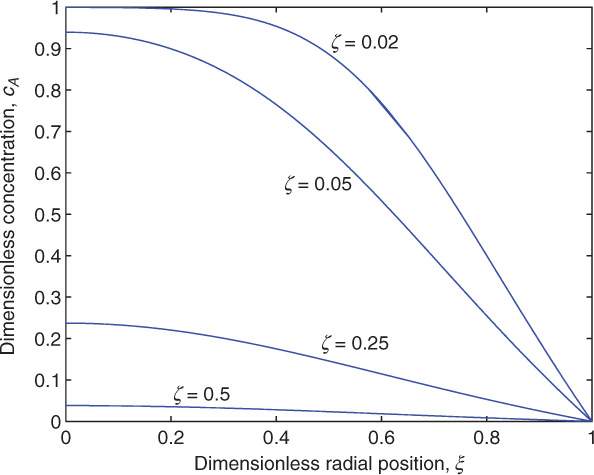
Figure 10.1 Concentration profile for Graetz problem as a function of radial position; the solution is shown at four axial locations, ζ .

The center concentration is often of interest since this is where the concentration has a maximum deviation from the value at the wall. The leading term in the solution for the center concentration is obtained from Equation 10.7 by setting ξ = 0 and taking n = 1:

c_A(ξ = 0) ≈ 0.9774 exp(–2.704²ζ)F₁(0)

This is called the one-term approximation. The value of F₁(0) is also tabulated in Table 10.1 for quick calculations of the center concentration and is equal to 1.5106. We find the mass transfer is almost complete at ζ = 0.5. For this length the value of the center concentration is 0.0381. The one-term solution should not be used near the entrance (ζ < 0.02 or so) as the concentration in the entry region is rather steep. More terms in the series should be used or an alternative similarity solution discussed in Section 10.2 is more suitable.

Local Sherwood Number

The quantity of primary engineering interest is usually the mass flux N_Ar or mass transfer rate to the wall. This is obtained by using Fick’s law at the wall:

\begin{matrix} N_{A r} = - D_{A} (\frac{\partial C_{A}}{\partial r})_{r = R} & (10.11) \end{matrix}

$\begin{matrix} N_{A r} = - D_{A} (\frac{\partial C_{A}}{\partial r})_{r = R} & (10.11) \end{matrix}$

The results are expressed in terms of a local mass transfer coefficient k_m defined as

N_Ar = k_m(C_Ab – C_As)

In this expression, C_Ab is the cup-mixing or flow-averaged concentraion, defined as

\begin{matrix} C_{A b} = \frac{\int_{0}^{R} 2 π r υ_{z} (r) C_{A} (r) d r}{\int_{0}^{R} 2 π r υ_{z} d r} & (10.12) \end{matrix}

$\begin{matrix} C_{A b} = \frac{\int_{0}^{R} 2 π r υ_{z} (r) C_{A} (r) d r}{\int_{0}^{R} 2 π r υ_{z} d r} & (10.12) \end{matrix}$

The mass flux to the wall or equivalently the mass transfer coefficient is expressed in dimensionless form in terms of the Sherwood number, defined as

\begin{matrix} S h = \frac{k_{m} d_{t}}{D_{A}} = \frac{d_{t} N_{A r}}{D_{A} (C_{A b} - C_{A s})} & (10.13) \end{matrix}

$\begin{matrix} S h = \frac{k_{m} d_{t}}{D_{A}} = \frac{d_{t} N_{A r}}{D_{A} (C_{A b} - C_{A s})} & (10.13) \end{matrix}$

From the relation for N_Ar given by Equation 10.11 the following expression for the Sherwood number is obtained:

\begin{matrix} S h = - \frac{2}{c_{A b}} (\frac{\partial c_{A}}{\partial ξ})_{ξ = 1} & (10.14) \end{matrix}

$\begin{matrix} S h = - \frac{2}{c_{A b}} (\frac{\partial c_{A}}{\partial ξ})_{ξ = 1} & (10.14) \end{matrix}$

Here c_Ab is the dimensionless cup-mixing average temperature, defined as

\begin{matrix} c_{A b} (ζ) = 4 \int_{0}^{1} ξ (1 - ξ^{2}) c_{A} d ξ & (10.15) \end{matrix}

$\begin{matrix} c_{A b} (ζ) = 4 \int_{0}^{1} ξ (1 - ξ^{2}) c_{A} d ξ & (10.15) \end{matrix}$

The mass flux to the wall and the corresponding local Sherwood number can be calculated by taking the derivative of the F function at the pipe wall and also by evaluating c_Ab (see Equation 10.15). The result for the local Sherwood number, after some clever algebra that avoids integration of the Kummer functions, is

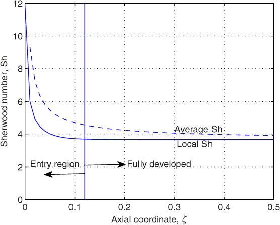
S h (ζ) = \frac{\sum_{n = 1}^{\infty} C_{n} F_{n}^{'} (1) exp (- λ_{n}^{2} ζ) F_{n}^{'} (1)}{\sum_{n = 1}^{\infty} 2 C_{n} [F_{n}^{'} (1) / λ_{n}^{2}] exp (- λ_{n}^{2} ζ)}

$S h (ζ) = \frac{\sum_{n = 1}^{\infty} C_{n} F_{n}^{'} (1) exp (- λ_{n}^{2} ζ) F_{n}^{'} (1)}{\sum_{n = 1}^{\infty} 2 C_{n} [F_{n}^{'} (1) / λ_{n}^{2}] exp (- λ_{n}^{2} ζ)}$

The first five numerical values of $F_{n}^{'}$ $F_{n}^{'}$ are also shown in Table 10.1 as a quick aid to calculation of the Sherwood number. For one-term approximation, the value of Sh reduces to $λ_{1}^{2} / 2$ $λ_{1}^{2} / 2$ . Hence the Sherwood number takes an asymptotic value of 3.657. The reader may wish to note that the entire calculation can be easily done in MALTAB with CHEBFUN as shown later in this chapter.

Average Sherwood Number

Note that the local Sherwood number will be a function of the axial position ζ. The quantity of interest, especially for the 1-D or mesoscopic model discussed in Section 4.2, is the average Sherwood number over a length L* of the pipe. This is defined as

\bar{S} h_{L} = \frac{1}{L *} \int_{0}^{L} S h d ζ

$\bar{S} h_{L} = \frac{1}{L *} \int_{0}^{L} S h d ζ$

The average Sherwood number over a length L* of pipe can be calculated by integration and is given as

\bar{S} h_{L} = 3.6 6 + \frac{0.0 668 P e / L *}{1 + 0.0 4 [P e / L *]^{2 / 3}}

$\bar{S} h_{L} = 3.6 6 + \frac{0.0 668 P e / L *}{1 + 0.0 4 [P e / L *]^{2 / 3}}$

where L* = L/d_t. As L* becomes large the average Sherwood number approaches an asymptotic value of 3.66.

A plot of the local and average Sherwood number as a function of the axial coordinate ζ is shown in Figure 10.2.

Graphical representation showing the local Sherwood number as a function of axial distance.

Figure 10.2 Plot of local Sherwood number as a function of axial distance.

10.2 Wall Reaction: The Robin Problem

A variation to the constant concentration problem is the Robin problem, which is applicable when there is a heterogeneous reaction at the wall. The reaction is assumed to follow first-order kinetics in this discussion so that the separation of variables method is applicable. Nonlinear kinetics require a numerical solution and the PDEPE code in Section 8.11 can be used for such cases. For linear reactions, the eigenproblem can be solved using CHEBFUN, which is illustrated in Section 10.2.1.

The wall boundary condition for a first-order surface reaction at the wall is obtained by balancing the flux to the wall (Fick’s law) to the rate at which A is consumed by the wall reaction:

- D_{A} (\frac{d C_{A}}{d r})_{r = R} = k_{s} C_{A} (r = R)

$- D_{A} (\frac{d C_{A}}{d r})_{r = R} = k_{s} C_{A} (r = R)$

The inlet condition is taken as C_A₀. The dimensionless concentration is now scaled by the inlet concentration and defined as $c_{A} = \frac{C_{A}}{C_{A i}}$ $c_{A} = \frac{C_{A}}{C_{A i}}$ . Note that the wall concentration is not used in this definition unlike the earlier problem, as this is unknown.

The wall boundary condition in dimensionless form is

\frac{\partial c_{A}}{\partial ξ} + D a_{w^{C} A} = 0 at ξ = 1

$\frac{\partial c_{A}}{\partial ξ} + D a_{w^{C} A} = 0 at ξ = 1$

where Da_w is the wall reaction Biot number defined as k_sR/D_A. The boundary condition is homogeneous, which is a requirement for application of direct separation of variables. The problem is linear and amenable to an analytical solution using separation of variables but the computation of eigenvalues and eigenfunctions are even more formidable than the classical Graetz problem. The computations can be completed more easily using CHEBFUN to extract the eigenvalues and simultaneously calculate the eigenfunctions; the code is shown next.

10.2.1 Solution Using CHEBFUN

The use of CHEBFUN for the transient diffusion problem was discussed in Section 8.10 and the process is similar here. The code listing for the Graetz and the wall reaction problems is shown in Listing 10.1. The statement A.rbc in the code needs to be changed accordingly for these two cases.

Listing 10.1 Solution of the Linear Convection-Diffusion Problem Using CHEBFUN

Click here to view code image

% CHEBFUN code for Graetz problem.
xi = chebfun(’xi’,[0,1]);
A = chebop(0,1);
A.op = @(xi,u) xi.*diff(u,2)+diff(u,1);
A.lbc = @(u) diff(u,1)   % Neumann
% % Dirichelt problem
A.rbc = @(u) u        % Dirichlet
% % Robin problem
Da = 1.0;
A.rbc = @(u) diff(u,1)+Da*u % Robin
B = chebop(0,1);
B.op = @(xi,u)–xi.*(1–xi.^2).*u ;
% then we find the eigenvalues with eigs
[F,L] = eigs(A,B)
omega = sqrt(diag(L)) % eigenvalues
% series coefficient can be evaluated
for i = 1:6
   N1 = int (xi.*(1–xi.^2).* F(:,i));
N2 = int (xi.*(1–xi.^2).* F(:,i).* F(:,i));
A1(i)= N1/N2 ;
end
% solution for a given axial distance
zeta1= 0.5; % axial distance parameter
% one term solution for comparison
i = 1
theta_c = A1(i)*exp(–omega(i)^2*zeta1)* F(xi,i)% answer 0.0381
  %  six term solution
sum = 0.0 ;
for i = 1:6
      sum = sum + A1(i)*exp(–omega(i)^2*zeta1)* F(xi,i) ;
end
c_zeta = sum % plot (c_zeta) %
plot of the solution
%% cup–mixing concentration
c_cup = 4* int(xi.*(1–xi.^2).* c_zeta)
%% local Sherwood number
Fdash = diff(c_zeta) % derivative of the concentration
Sh =–2.* Fdash(1)/c_cup % answer = 3.6568.for Graetz

10.2.2 Illustrative Results

Some illustrative results for the Sherwood number and wall concentration at four axial locations are shown in Table 10.2 for three values of the wall Biot number. A point worth noting is that for low values of Da_w the asymtotic value of the Sherwood number approaches 4.36. This represents a case of constant mass input to the wall (constant flux condition at the wall) and the result can also be proved from a theoretical analysis. At high values of Da_w, the Sherwood number approaches an asymptotic value of 3.66, the constant concentration asymptote.

Table 10.2 Results for First-Order Wall Reaction

ζ	0.0500	0.2500	0.5000	1.0000
		Da_w = 0.1
Sh, local	4.9402	4.3339	4.3309	4.3309
c_A(ξ = 1)	0.9427	0.8685	0.7893	0.6519
		Da_w = 1.0
Sh, local	4.7178	4.1264	4.1242	4.1242
c_A(ξ = 1)	0.6044	0.3368	0.1717	0.0447
		Da_w = 10
Sh, local	4.1947	3.7633	3.7629	3.7629
c_A(ξ = 1)	0.1117	0.0283	0.0058	0.0002

The concentration profile is shown in Figure 10.3 at an axial location of ζ = 0.25 as a function of the radial position.

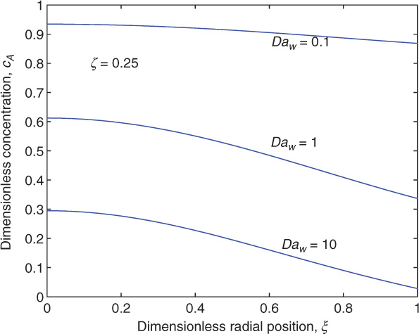
Figure 10.3 Concentration profile for the wall reaction problem as a function of radial position; the solution is shown at axial location ζ of 0.25 for three values of the wall Biot number.

The key points to note are the following. At low values of Da_w, there is no significant radial variation and mass transfer effects are not important. The reaction resistance is dominant. At higher values of Da_w the profiles are steep and the wall concentration tends to zero. This represents a case where the mass transfer to the wall is the dominant resistance.

10.3 Entry Region Analysis

Application of the series solution described in Section 10.1.2 requires a large number of terms for small values of ζ , that is, near the entrance region. The reason is that the concentration profile is rather steep and confined to a region near the wall. Much of the core fluid remains at the inlet concentration. Hence an alternative method is to seek a similarity solution similar to the error function solution discussed for transient mass transfer.

The starting differential equation 10.6 is rewritten, expanding the Laplacian as

\begin{matrix} (1 - ξ^{2}) \frac{\partial c_{A}}{\partial ζ} = \frac{\partial^{2} c_{A}}{\partial ξ^{2}} + \frac{1}{ξ} \frac{\partial θ}{\partial ξ} & (10.16) \end{matrix}

$\begin{matrix} (1 - ξ^{2}) \frac{\partial c_{A}}{\partial ζ} = \frac{\partial^{2} c_{A}}{\partial ξ^{2}} + \frac{1}{ξ} \frac{\partial θ}{\partial ξ} & (10.16) \end{matrix}$

The distance from the wall, defined as s* = 1 – ξ, is now more convenient. The velocity profile term 1 – ξ² is now approximated as 2s*, that is, we keep only the linear term. Also we keep only the first term for the Laplacian. Thus the second term on the right-hand side is dropped. This amounts to ignoring the curvature effects and representing the geometry using simpler rectangular coordinates.

The differential equation now is

\begin{matrix} 2 s * \frac{\partial c A}{\partial ζ} = \frac{\partial^{2} c A}{\partial s *^{2}} & (10.17) \end{matrix}

$\begin{matrix} 2 s * \frac{\partial c A}{\partial ζ} = \frac{\partial^{2} c A}{\partial s *^{2}} & (10.17) \end{matrix}$

We find that 2s*³/ζ should be used as a similarity variable (or its cube root) since there is no well-defined length scale in the entry region. Note that the radius of the pipe is not a relevant length scale here as the concentration changes are now confined to a thin region near the wall. It is now convenient to use a similarity variable defined as

η = s * (\frac{2}{9 ζ})^{1 / 3} or = s * {(\frac{2 P e}{9 z *})}^{1 / 3}

$η = s * (\frac{2}{9 ζ})^{1 / 3} or = s * {(\frac{2 P e}{9 z *})}^{1 / 3}$

The factor 2/9 is included for the convenience of a simplified form of the results at the end.

The differential equation 10.17 now reduces to an ordinary differential equation in terms of the similarity variable η:

\begin{matrix} \frac{d^{2} c_{A}}{d η^{2}} + 3 η^{2} \frac{d c_{A}}{d η} = 0 & (10.18) \end{matrix}

$\begin{matrix} \frac{d^{2} c_{A}}{d η^{2}} + 3 η^{2} \frac{d c_{A}}{d η} = 0 & (10.18) \end{matrix}$

The boundary conditions to be used now are as follows. At η = 0, the wall, c_A = 0. At η → ∞, the center or the inlet, c_A = 1. We also note that the three conditions merge into two, which is a characteristic of similarity solution methods.

The solution is found by integrating this equation twice. The first integration gives an expression for the concentration gradient. A second integration gives the concentration profile. The details are left as an exercise. The second integration has no closed analytical form and the final answer is expressed in terms of the incomplete gamma function:

\begin{matrix} \begin{matrix} Entry region : c_{A} = \frac{1}{Γ (4 / 3)} \int_{0}^{η} exp (- t^{3}) d t \end{matrix} & (10.19) \end{matrix}

$\begin{matrix} \begin{matrix} Entry region : c_{A} = \frac{1}{Γ (4 / 3)} \int_{0}^{η} exp (- t^{3}) d t \end{matrix} & (10.19) \end{matrix}$

where η is the similarity variable defined earlier and t is a dummy variable for integration. Equation 10.19 is also known as the Leveque solution.

The results can be expressed compactly as an incomplete gamma function as c_A = gammainc(η³, 1/3), which is readily calculated in MATLAB. A plot of the incomplete gamma function is presented in Figure 10.4 as an aid to quick calculations.

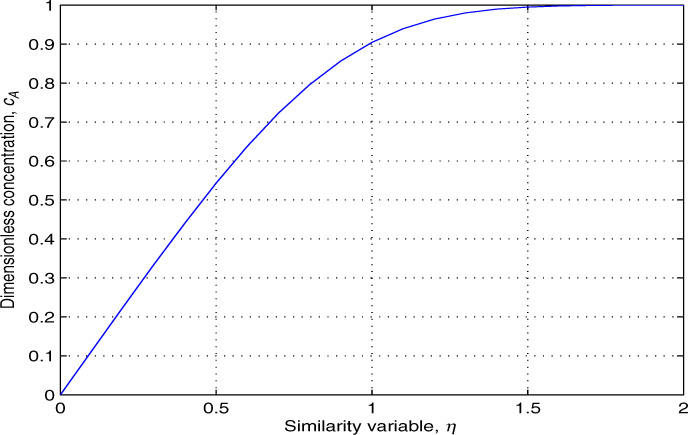
Graphical representation of the incomplete gamma function.

Figure 10.4 Plot of concentration profile for the entry region as a function of the similarity variable. This is a plot of gammainc(η³, 1/3).

The corresponding local mass flux is calculated as

\begin{matrix} N_{A w} \frac{R}{D_{A}} = [\frac{(2 P e / z *)^{1 / 3}}{9^{1 / 3} Γ (4 / 3)}] (C_{A s} - C_{A, i}) & (10.20) \end{matrix}

$\begin{matrix} N_{A w} \frac{R}{D_{A}} = [\frac{(2 P e / z *)^{1 / 3}}{9^{1 / 3} Γ (4 / 3)}] (C_{A s} - C_{A, i}) & (10.20) \end{matrix}$

Rearranging and basing the Sherwood number on diameter we have

\begin{matrix} S h = 1.0 77 (2 P e / z *)^{1 / 3} & (10.21) \end{matrix}

$\begin{matrix} S h = 1.0 77 (2 P e / z *)^{1 / 3} & (10.21) \end{matrix}$

Note that the driving force for mass transfer is taken as (C_As – C_A,i) rather than (C_Ab – C_A,i) in the definition of the Sherwood number. This was also mentioned earlier in Chapter 9.

The Graetz number parameter, defined as Q/(D_Az), is used in laminar mass transfer literature, where Q is the volumetric flow rate. Thus turns out to be equal to Gz = (π/4)(2Pe/z*). Using this in Equation 10.21, the Sherwood number in the entry region can also be expressed in terms of the Graetz number as

\begin{matrix} S h = 1.8 77 G z^{1 / 3} & (10.22) \end{matrix}

$\begin{matrix} S h = 1.8 77 G z^{1 / 3} & (10.22) \end{matrix}$

10.4 Channel Flows with Mass Transfer

In this section, we examine briefly the problem of convective mass transfer with flow between two parallel plates. Flow is in the x-direction. The plate surfaces are at y = ±h, that is, h is half the gap width. y = 0 represents the center and is a plane of symmetry. The plates are assumed to be long in the z-direction (perpendicular to the x-y plane) and hence the problem is solved in Cartesian x-y coordinates. The governing equation is

\begin{matrix} υ_{x} \frac{\partial C_{A}}{\partial x} = D_{A} \frac{\partial^{2} C_{A}}{\partial y^{2}} & (10.23) \end{matrix}

$\begin{matrix} υ_{x} \frac{\partial C_{A}}{\partial x} = D_{A} \frac{\partial^{2} C_{A}}{\partial y^{2}} & (10.23) \end{matrix}$

The diffusion in the axial (x) direction is ignored in the above model. Thus the convection in the x-direction balances the diffusion in the y-direction.

The velocity profile in channel flow is given from fluid mechanics as

υ_{x} = υ_{max} [1 - (\frac{y}{h})^{2}] = \frac{3}{2} 〈 υ 〉 [1 - (\frac{y}{y})^{2}]

$υ_{x} = υ_{max} [1 - (\frac{y}{h})^{2}] = \frac{3}{2} 〈 υ 〉 [1 - (\frac{y}{y})^{2}]$

The flow is assumed to be fully developed here and the fluid to be Newtonian. Note that the maximum velocity is 3/2 times the average velocity in channel flow.

Equation 10.23 reduces to the following when dimensionless variables are used:

\begin{matrix} \frac{3}{2} (1 - ξ^{2}) \frac{\partial c_{A}}{\partial ζ} = \frac{\partial^{2} c_{A}}{\partial ξ^{2}} & (10.24) \end{matrix}

$\begin{matrix} \frac{3}{2} (1 - ξ^{2}) \frac{\partial c_{A}}{\partial ζ} = \frac{\partial^{2} c_{A}}{\partial ξ^{2}} & (10.24) \end{matrix}$

The parametric representation is now

c_A = c_A(ζ, ξ)

The ζ is the dimensionless coordinate in the flow direction, defined as

β = \frac{4 (x / h)}{ReSc}

$β = \frac{4 (x / h)}{ReSc}$

The Reynolds number is defined based on the hydraulic diameter, which is equal to 4h:

R e = \frac{4 h 〈 υ 〉}{ν}

$R e = \frac{4 h 〈 υ 〉}{ν}$

Equation 10.24 has the series solution similar to that for pipe flow (Equation 10.7), which is reproduced below for ease of reference:

\begin{matrix} c_{A} (ζ, ξ) = \sum_{n = 1}^{\infty} C_{n} exp (- λ_{n}^{2} ζ) F_{n} (ξ) & (10.25) \end{matrix}

$\begin{matrix} c_{A} (ζ, ξ) = \sum_{n = 1}^{\infty} C_{n} exp (- λ_{n}^{2} ζ) F_{n} (ξ) & (10.25) \end{matrix}$

However, the eigenvalues and so on are now different since the diffusion operator is now in Cartesian coordinates rather than in cylindrical coordinates. These can be generated easily using the CHEBFUN code shown in Listing 10.2.

Listing 10.2 CHEBFUN for Eigenvalues and Eigenfunctions for Channel Flow Mass Transfer

Click here to view code image

xi = chebfun(’xi’,[0,1]);
A = chebop(0,1);
A.op = @(xi,u) diff(u,2);
A.lbc = @(u) diff(u,1) % Neumann
A.rbc = @(u) u % Dirichlet

B = chebop(0,1);
B.op = @(xi,u)–3/2*(1–xi.^2).*u ;
%%
neig = 6 % first six values
[F,L ] = eigs(A,B, neig)

The square of the eigenvalues is found in the diagonal L while the eigenfunctions are found in F as Chebechev polynominals. The series coefficients are then calculated using the code segment shown in Listing 10.3. Note that the eigenfunctions are now orthogonal with a weighting factor of 1 – ξ².

Listing 10.3 Code to Find Series Coefficients for Channel Flow

Click here to view code image

i = 1:neig
N1 = int ((1–xi.^2).* F(:,i));
N2 = int ((1–xi.^2).* F(:,i).* F(:,i));
A1(i)= N1/N2 ;
B1(i) = N1
C1(i) = A1(i)*B1(i)*3/2
end

The solution can now be calculated using Equation 10.25. Once the concentration distribution is known, the Sherwood number is calculated as

S h = \frac{4 h k_{m}}{D_{A}} = - \frac{4 (\partial c_{A} / \partial ξ)_{ξ = 0}}{c_{A b}}

$S h = \frac{4 h k_{m}}{D_{A}} = - \frac{4 (\partial c_{A} / \partial ξ)_{ξ = 0}}{c_{A b}}$

where c_Ab is the dimensionless cup-mixing concentration defined as

c_{A b} = \frac{3}{2} \int_{0}^{h} (1 - ξ^{2}) c_{A} (ξ) d ξ)

$c_{A b} = \frac{3}{2} \int_{0}^{h} (1 - ξ^{2}) c_{A} (ξ) d ξ)$

Note that the hydraulic diameter (4h) is again used as the length scale. The plot of the Sherwood number as a function of axial distance is shown in Figure 10.5.

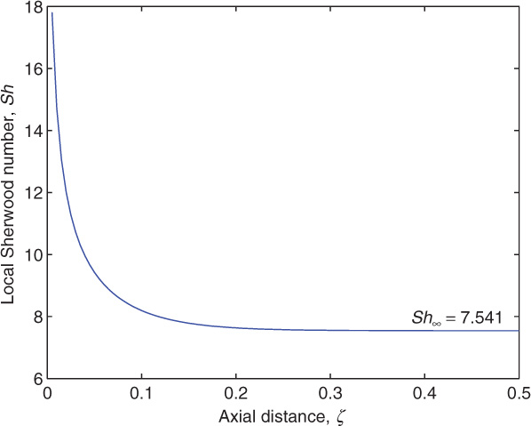
Graphical illustration of the Mass transfer coefficient as a function of axial distance.

Figure 10.5 Mass transfer coefficient (Sherwood number) for flow in a channel with constant wall concentration.

The Sherwood number reaches an asymptotic value of 7.541. Laminar flow holds until a Reynolds number of 2800 for channel flows and the model is not applicable in turbulent flow conditions.

The case of wall reaction can also be easily generated using the CHEBFUN-MATLAB code. Details are not presented here since it is an extension of the corresponding scheme for pipe flows.

10.5 Mass Transfer in Film Flow

An important class of problems involves mass transfer to or from a liquid flowing as a thin film over a vertical plate. The velocity profile for film flow is obtained by balancing the gravity forces with viscous forces. The result from fluid dynamic literature for laminar flow of the film is

\begin{matrix} υ_{z} (y) = \frac{ρ g}{μ} [δ y - \frac{y^{2}}{2}] & (10.26) \end{matrix}

$\begin{matrix} υ_{z} (y) = \frac{ρ g}{μ} [δ y - \frac{y^{2}}{2}] & (10.26) \end{matrix}$

Here z is the flow direction, (vertically downward for film flow over a vertical wall). The y is the cross-flow direction starting from the wall. The laminar flow assumption is valid if the Reynolds number based on film thickness and average velocity is less than 20.

The film thickness δ can be computed from an overall integral mass balance (integral from 0 to y) and is related to the liquid flow rate Q/W (per unit width of the wall) as follows:

δ = \sqrt[3]{\frac{3 μ Q / W}{ρ g}}

$δ = \sqrt[3]{\frac{3 μ Q / W}{ρ g}}$

Now we analyze the mass transport of a species dissolving from the wall or absorbed from the interface into the film.

10.5.1 Solid Dissolution at a Wall in Film Flow

The governing equation for mass transfer in film flow is

\begin{matrix} υ_{z} (y) \frac{\partial C_{A}}{\partial z} = D \frac{\partial^{2} C_{A}}{\partial y^{2}} & (10.27) \end{matrix}

$\begin{matrix} υ_{z} (y) \frac{\partial C_{A}}{\partial z} = D \frac{\partial^{2} C_{A}}{\partial y^{2}} & (10.27) \end{matrix}$

Here we neglect diffusion in the flow direction. Thus the left-hand side represents convection in the direction of flow (z) and the right-hand side represents diffusion in the cross-flow direction (y). The Sc, defined as ν/D, is the key parameter affecting the mass transfer penetration distance. For liquids, the Sc is large and we expect a boundary layer type of concentration distribution; the solute concentration changes will be confined to only a small part of the hydrodynamic film thickness.

Anticipating a concentration boundary layer near the wall, we use a linearized form as an approximation for the velocity. The approximation is shown in Figure 10.6:

υ_z = βy

A thick, vertical line is drawn denoting the "Wall coated with a solute." A thin, dotted line is drawn to the right of the wall, and the distance between the two lines is labeled "Film thickness, Delta." The Liquid flow is from the top to the bottom, and the Mass transfer is through the wall from left to right. At the top, two arrows indicate the directions, y denotes the mass transfer direction and the z denotes the liquid flow direction. A dotted line is drawn along the film's thickness. The velocity of the liquid flow is v subscriptz. A decreasing curve is drawn from the point where the dotted line originates at the wall, and the curve gradually decreases to cease at a lower point on the dotted line. Three arrows denoting the liquid flow are drawn from the horizontal dotted line and they touch and stop at the curve. A slanted dotted line that coincides with the curve is shown.

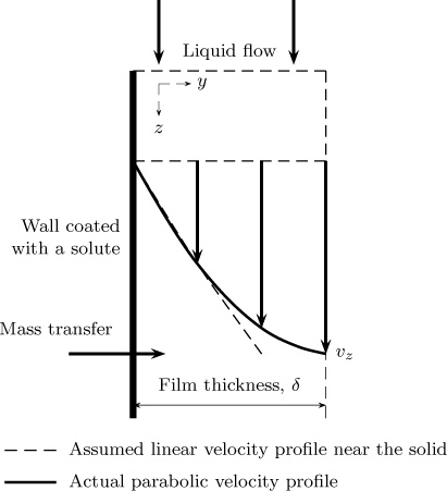
Figure 10.6 Solid dissolution in film flow. In the solid dissolution case, the region near the wall is important.

where β is the slope of the velocity profile near the wall, given as

β = \frac{ρ g}{μ} δ

$β = \frac{ρ g}{μ} δ$

This will be the velocity profile “seen” by the diffusing species and hence the convection-diffusion model (Equation 10.27) reduces to

\begin{matrix} β y \frac{\partial C_{A}}{\partial z} = D \frac{\partial^{2} C_{A}}{\partial y^{2}} & (10.28) \end{matrix}

$\begin{matrix} β y \frac{\partial C_{A}}{\partial z} = D \frac{\partial^{2} C_{A}}{\partial y^{2}} & (10.28) \end{matrix}$

The domain of the solution is set as semi-infinite since the concentration profile is assumed to be confined to a thin region near the wall. A similarity variable η is defined as follows:

η = y (\frac{β}{9 D z})^{1 / 3}

$η = y (\frac{β}{9 D z})^{1 / 3}$

With this transformation, Equation 10.28 reduces to an ordinary differential equation for the dimensionless concentration as a function of η:

\begin{matrix} \frac{d^{2} c_{A}}{d η^{2}} + 3 η^{2} \frac{d c_{A}}{d η} = 0 & (10.29) \end{matrix}

$\begin{matrix} \frac{d^{2} c_{A}}{d η^{2}} + 3 η^{2} \frac{d c_{A}}{d η} = 0 & (10.29) \end{matrix}$

The inlet condition and the condition as y → ∞ merge into a single condition that states that at η = ∞, c_A = 0.

The wall boundary condition is the second boundary condition and at η = 0, c_A = 1.

The solution to Equation 10.29 with these boundary conditions can be derived as

\begin{matrix} \frac{C_{A}}{C_{A s}} = 1 - \frac{\int_{0}^{η} exp (- η^{3} d η}{Γ (4 / 3)} & (10.30) \end{matrix}

$\begin{matrix} \frac{C_{A}}{C_{A s}} = 1 - \frac{\int_{0}^{η} exp (- η^{3} d η}{Γ (4 / 3)} & (10.30) \end{matrix}$

The solution can be readily computed using the built-in function in MATLAB as

\begin{matrix} \frac{C_{A}}{C_{A s}} = 1 - gammainc (η^{3}, 1 / 3) & (10.31) \end{matrix}

$\begin{matrix} \frac{C_{A}}{C_{A s}} = 1 - gammainc (η^{3}, 1 / 3) & (10.31) \end{matrix}$

which gives the dimensionless concentration as a function of η . The concentration profile is shown in Figure 10.7 where a comparison with the numerical solution is also shown.

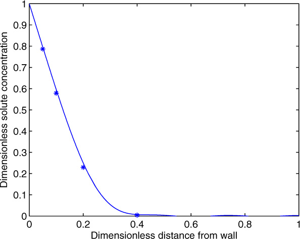
Figure 10.7 Concentration profile for solid dissolution in a falling film and comparison of the similarity solution with the numerical solution, marked with *.

The local rate of mass transfer is obtained using Fick’s law at the wall:

N_{A} = \frac{D C_{A s}}{Γ (4 / 3)} (\frac{β}{9 D z})^{1 / 3}

$N_{A} = \frac{D C_{A s}}{Γ (4 / 3)} (\frac{β}{9 D z})^{1 / 3}$

The average rate of mass transfer over a length L is given by

{\bar{N}}_{A} = \frac{2 D C_{A s}}{Γ (7 / 3)} (\frac{β}{9 D L})^{1 / 3}

${\bar{N}}_{A} = \frac{2 D C_{A s}}{Γ (7 / 3)} (\frac{β}{9 D L})^{1 / 3}$

If one divides this by C_As, the driving force, one can calculate the average value of the mass transfer coefficient over a length L:

k_{s l} = \frac{2}{Γ (7 / 3)} D^{2 / 3} β^{1 / 3} L^{- 1 / 3}

$k_{s l} = \frac{2}{Γ (7 / 3)} D^{2 / 3} β^{1 / 3} L^{- 1 / 3}$

The model can be extended to film flow of non-Newtonian fluids. The corresponding velocity profile is to be included. Mashelkar and Chavan (1973) provide the results for solid dissolution mass transfer for pseudoplastic fluids.

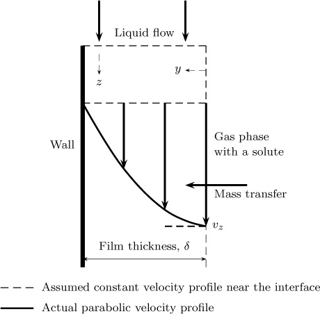
10.5.2 Gas Absorption from Interface in Film Flow

Here we consider the mass transfer of a species present in the gas into the liquid film. Again a concentration boundary layer is proposed near the interface. The velocity profile seen is now flat and equal to υ_max rather than a linear profile as in the previous subsection. The maximum velocity in turn is given from Equation 10.26 by setting y = δ and is

υ_{max} = \frac{ρ g δ^{2}}{2 μ}

$υ_{max} = \frac{ρ g δ^{2}}{2 μ}$

The diffusing species now sees this flat velocity profile rather than the full parabolic profile. This is also illustrated in Figure 10.8.

Diagrammatic representation shows gas absorption in film flow.

A thick, vertical line is drawn denoting the "Wall." A thin, dotted line is drawn to the right of the wall, and the distance between the two lines is labeled "Film thickness, Delta." The Liquid flow is from the top to the bottom, the Mass transfer is through the film from right to left. At the top, two arrows indicate the directions, y denotes the mass transfer direction and the z denotes the liquid flow direction. A dotted line is drawn along the film's thickness. The velocity of the liquid flow is v subscriptz. A decreasing curve is drawn from the point where the dotted line originates at the wall, and the curve gradually decreases to cease at a lower point on the dotted line. Three arrows denoting the liquid flow are drawn from the horizontal dotted line and they touch and stop at the curve.

Figure 10.8 Gas absorption in film flow: the region near the interface is important.

The convection-diffusion equation can now simplified by using υ_z as a constant equal to υ_max:

\begin{matrix} υ_{max} \frac{\partial C_{A}}{\partial z} = D \frac{\partial^{2} C_{A}}{\partial y^{2}} & (10.32) \end{matrix}

$\begin{matrix} υ_{max} \frac{\partial C_{A}}{\partial z} = D \frac{\partial^{2} C_{A}}{\partial y^{2}} & (10.32) \end{matrix}$

Note that the left-hand side of Equation 10.32 has no functional dependence on y and therefore the problem is closer to the transient diffusion problem rather than a convection-diffusion problem. In fact z/υ_max is a time-like variable and represents the exposure time of an element of fluid moving down the interface. The concentration profile is now represented in terms of an error function:

\begin{matrix} \frac{C_{A}}{C_{A s}} = 1 - erf (\frac{y}{\sqrt{4 D z / υ_{max}}}) & (10.33) \end{matrix}

$\begin{matrix} \frac{C_{A}}{C_{A s}} = 1 - erf (\frac{y}{\sqrt{4 D z / υ_{max}}}) & (10.33) \end{matrix}$

Here y is the now defined as the distance measured from the interface.

The local rate of mass transfer is obtained by using Fick’s law at the wall. The result is the same as the penetration theory model discussed in Section 8.8 with t replaced by the exposure time, which is equal to z/υ_max:

N_{A} = C_{A s} \sqrt{\frac{D υ_{max}}{π z}}

$N_{A} = C_{A s} \sqrt{\frac{D υ_{max}}{π z}}$

The average mass transfer coefficient over a length L is given as

\begin{matrix} \begin{matrix} k_{L} = 2 \sqrt{\frac{D υ_{max}}{π L}} \end{matrix} & (10.34) \end{matrix}

$\begin{matrix} \begin{matrix} k_{L} = 2 \sqrt{\frac{D υ_{max}}{π L}} \end{matrix} & (10.34) \end{matrix}$

This is again the same as the penetration theory model with the contact time set as L/υ_max.

10.6 Numerical Solution with PDEPE

The PDEPE program shown in Section 8.11 is a useful tool to simulate these classes of problems as well. A brief discussion is provided together with sample results for the Graetz problem.

This problem is readily handled by PDEPE by simply defining the capacity term as a function of radial position. In the notation used in the sample code, shown in Section 8.11, x represents dimensionless radial position, ξ, while t represents the dimensionless axial position η . The capacity term is now defined as

C = 1 – x²

in order to match Equation 10.6. The geometry parameter s should be set as one for pipe flow to match the Laplacian in cylindrical geometry. Setting it to zero will solve the channel flow case.

A sample code file graetz.m can be written with these modifications of the code for transient diffusion shown in Section 8.11.1.

Some results are given in Table 10.3 so that students can benchmark the programs and verify the results. The results are also shown for the case of constant wall concentration examined in Section 10.1.1.

Table 10.3 Results for the Graetz Problem Simulated with PDEPE

ζ	*1 – c_A(₀)*	*N_Ar*	1 – c_Ab	Sh
.05	0.0605	1.158	0.4213	4.00
0.1	0.2988	0.733	0.6047	3.71
0.15	0.5081	0.501	0.7265	3.665
0.20	0.6582	0.347	0.8103	3.658
0.25	0.7628	0.241	0.8684	3.657
0.30	0.8355	0.167	0.9087	3.657
0.35	0.8858	0.116	0.93679	3.657
0.40	0.9208	0.0803	0.9561	3.657

The value from the one-term solution for ζ = 0.4 is 0.9207 for the center concentration, which matches well with the PDEPE-generated solution shown in this table.

The Robin problems, nonlinear rate, and other cases can be easily handled by this procedure. Only the boundary conditions need to be modified. For channel flow we set the s parameter to zero.

The advantage of PDEPE over the CHBEBFUN method is that it can handle nonlinear boundary conditions. For linear problems the CHEBFUN method is most accurate since there is no spatial or time discretization.

Summary

Mass transfer from the walls to a fluid in a pipe under laminar flow conditions is the most widely studied problem in convective mass transfer. A number of assumptions are usually made to simplify the problem, such as constant viscosity and fully developed flow. Even then the problem is mathematically complicated and results in a partial differential equation in r and z with a variable coefficient term. The variable coefficient arises due to the velocity variation in the r direction. It is useful to understand the mathematical structure of the model equation.
The boundary condition at the wall can be of constant concentration (first kind or Dirichlet) or given by a wall reaction case (third kind or Robin). A series solution can be obtained for both cases. It is straightforward for the constant wall temperature case but the eigenfunctions are not simple well-known common functions; they to a class of functions called hyper-geometric functions. These functions can however be readily evaluated in MATLAB or MAPLE or CHEBFUN.
From a mesoscale modeling point of view the local and average value of the transfer coefficient are needed. These can be predicted from the detailed concentration profiles based on the differential model. The results are expressed in terms of a dimensionless group, the Sherwood number. The Sherwood number is an function of axial distance and decreases with distance, reaching an asymptotic value for large distances from the entrance.
The convergence of the series is rather poor near the entrance. An alternative method can be used here where we visualize a concentration boundary layer near the wall and hence it is more convenient to obtain the similarity solution for the entry region.
The effect of wall reaction can be analyzed by changing the wall boundary condition from Dirichlet to Robin. The eigenvalues can be obtained by using the CHEBFUN routine and the Sherwood number in the presence of a reaction can be computed.
Mass transfer in channel flow from dissolving walls is a similar problem and can be solved by the separation of variables method. Again CHEBFUN can be used to obtain the full solution without any mathematical pain.
Mass transfer into a falling film is an important problem in convective mass transfer. Solid dissolution at the walls and gas absorption at the interface are the two important prototype problems. The length of the wall (absorber) is usually small and hence an asymptotic entry region type of model is generally used for these cases. The local and average value of the mass transfer coefficient can be predicted from such a model. It is important to note the dependency on the diffusion coefficient. In the solid dissolution case the dependency is to the power of 2/3 while in the gas absorption case it is 1/2.
The PDEPE software studied in Chapter 8 is a useful tool for convective mass transport problems as well. Only minor code adjustments are needed to match the PDE being solved and the appropriate boundary condition. The use of this was demonstrated for the classical Graetz problem and the results for other cases can be similarly computed.

Review Questions

10.1 What is hydrodynamic entry length? Is the velocity unidirectional in this region?

10.2 What is the definition of a contracted axial distance parameter?

10.3 What is the asymptotic value of the Sherwood number for constant wall conditions?

10.4 What is the contracted length for which the mass transfer is nearly complete?

10.5 What is the asymptotic value of the Sherwood number for constant mass removal conditions, for example, a zero-order reaction at the wall?

10.6 How is the wall Biot number defined?

10.7 Does the Sherwood number increase or decrease with the wall reaction Biot number?

10.8 What is the dependency of the mass transfer coefficient on the mass flow rate in the entry region?

10.9 How does the mass transfer coefficient vary with axial length in the entry region?

10.10 What is the definition of the Graetz number?

10.11 What is the dependency of the mass transfer coefficient with diffusivity at a no-slip boundary?

10.12 What is the dependency of the mass transfer coefficient with diffusivity at a no-shear boundary?

Problems

10.1 Eigenvalues with CHEBFUN. Run the code given in Listing 10.1 and generate the results shown in Table 10.1 for the Dirichlet problem. Modify and run the code with a wall reaction and generate the results shown in Table 10.2. Run the code shown in Listing 10.2 for channel flow and verify the results in Figure 10.5. Extend the channel flow code for a linear wall reaction and plot Sh as a function of Damkohler number. Choose any fixed axial position for this plot.

10.2 Subliming wall. Water is flowing in a laminar flow reaction in a 1 cm diameter tube coated with benzoic acid. The value of D = 1 × 10^–9 m²/2. The velocity is 10 cm/sec. Calculate and plot the mass transfer coefficient as a function of axial position in the pipe. If the pipe is 3 m long, plot the solute concentration at the exit as a function of radius. Find the cup-mixing concentration and compare the results with the mesoscopic model given in Section 4.2.

10.3 Laminar flow with wall reaction. Find the exit concentration and the conversion for a laminar flow with wall reactor under the following conditions: fluid properties are similar to that for water; radius = 1 cm; length = 500 cm; mass flow rate = 0.1 kg/s; surface reaction constant k_s = 2 × 10^–4 m/s.

10.4 Mass transfer under constant wall flux conditions. A constant wall flux boudary condition is applied if there is a constant mass removal rate at the walls. For example if a zero-order reaction is taking place, the wall boundary condition can be stated as follows: show that the wall boundary condition in dimensionless form is

\frac{\partial c_{A}}{\partial ξ} = - D a_{w 0} at ξ = 1

$\frac{\partial c_{A}}{\partial ξ} = - D a_{w 0} at ξ = 1$

Here Da_w₀ is the wall reaction Biot number for a zero-order wall reaction. How is this defined?

The asymptotic value of the mass transfer can be derived by the following procedure. Assume that the dimensionless concentration is linear invariant in the axial direction and propose a solution of the form

c_A = Aζ + F (ξ)

where A is a constant. Substitute this in Equation 10.6 and derive an equation for F . Integrate this equation to find F with the boundary condition at the wall and the center. Find the cup-mixing concentration and use this in the definition for Sherwood number given by Equation 10.13. Show that the resulting value of the asymptotic Sherwood number is 48/11, which is is a classic result.

10.5 Solid dissolution in a falling film. Consider a liquid flowing down a vertical wall at a rate of 1 × 10^–5 m²/s per meter unit width. Find the concentration at a height 25 cm below the entrance for a dissolving wall such as a wall coated with benzoic acid as a function of distance from the wall. Also find the local mass transfer coefficient.

Find the average mass transfer coefficient for a 50 cm wall. Assume D = 2 × 10^–9 m²/s and other properties similar to that of water. Use C_As = 20 mol/m³.

10.6 Gas absorption in a falling film. Repeat the analysis from problem 5 if instead, a gas such as oxygen is being absorbed into the liquid film.

10.7 Laminar flow and mass transfer for a power law fluid. Extend the analysis of the laminar flow mass transfer in Section 10.1 for a power law liquid. The velocity profile is now given as

\begin{matrix} υ_{z} = \frac{3 n + 1}{n + 1} 〈 υ 〉 [1 - (\frac{r}{R})^{(n + 1) / n}] & (10.35) \end{matrix}

$\begin{matrix} υ_{z} = \frac{3 n + 1}{n + 1} 〈 υ 〉 [1 - (\frac{r}{R})^{(n + 1) / n}] & (10.35) \end{matrix}$

where n is the power law index. Perform some computations using the PDEPE solver and show how the power law index affects the mass transfer coefficient.

10.8 Mass transfer in a counterflow exchanger. A feed solution containing a solute enters the inner tube of a mass exchanger. A membrane separates the inner tube with an annular outer cylinder. The solute diffuses across the membrane into the annular region. A sweep solution enters from the other side in the annular section and carries away the diffusing solute. The schematic is presented in Figure 10.9. The problem is representative of transport across dialysis equipment.

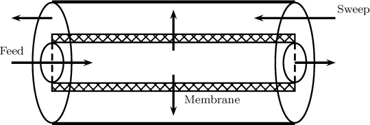
Diagrammatic representation of the problem related to mass transfer in a counterflow exchanger.

Figure 10.9 Mass transfer in a counterflow mass exchanger.

Assume laminar flow in both the inner and outer pipe. Set up the convection-diffusion model for both the inner pipe and the annular pipe. Set up the boundary conditions showing all the details clearly.

10.9 Mass transfer in oscillating flow. Mass transfer can be enhanced by flow oscillation. Assume that the flow oscillation is caused by a sinusoidal variation of the inlet pressure. Perform a scaling analysis based on the key time constants to find conditions under which the enhancement is likely and also investigate the problem using numerical tools such as PDEPE. Determine how the time-averaged Sherwood number varies with the dimensionless amplitude of oscillation.

..................Content has been hidden....................

You can't read the all page of ebook, please click here login for view all page.

Table of Contents for Chapter 10. Convective Mass Transfer: Theory for Internal Laminar Flow

Create new playlist

Sign In

Sign Up

Chapter 10. Convective Mass Transfer: Theory for Internal Laminar Flow

10.1 Mass Transfer in Laminar Flow in a Pipe

10.1.1 Dimensionless Form

Simplification for Large Peclet Number

10.1.2 Constant Wall Concentration: The Dirichlet Problem

10.1.3 Concentration, Wall Mass Flux, and Sherwood Number

Local Sherwood Number

Average Sherwood Number

10.2 Wall Reaction: The Robin Problem

10.2.1 Solution Using CHEBFUN

10.2.2 Illustrative Results

10.3 Entry Region Analysis

10.4 Channel Flows with Mass Transfer

10.5 Mass Transfer in Film Flow

10.5.1 Solid Dissolution at a Wall in Film Flow

10.5.2 Gas Absorption from Interface in Film Flow

10.6 Numerical Solution with PDEPE

Summary

Review Questions

Problems

Table of Contents for
Chapter 10. Convective Mass Transfer: Theory for Internal Laminar Flow