
Chapter 28. Liquid Separation Membranes
Learning Objectives
After completing this chapter, you will be able to:
Classify liquid membrane separation processes based on the pore size.
Understand the concepts of osmosis and reverse osmosis.
Model the transport of solvent and solute species across a semi-permeable membrane.
Examine the concentration polarization effect on the transport rate.
Develop a simplified model for design of a reverse osmosis system.
Understand forward osmosis separation and its application.
Calculate the extent of separation in a pervaporation process.
Separation of liquid mixtures using membranes finds application in many areas. An important application is in wastewater treatment and providing drinking water using desalination. Membranes selective to water transport that exclude the solute are used to purify the water, a process known as reverse osmosis. Other applications include separation of low molecular solutes such as enzymes from fermentation broths, and separation of biobased products such vitamins. The process finds application in the food industry as well in concentration of fruit juices and similar applications.
Transport and separation of components in a liquid mixture by use of membranes is discussed first in this chapter. We classify separation systems based on the pore size of membranes. For micro-sized pores, concepts borrowed from filtration or flow through a capillary can be used. For nano-sized pores, diffusion-based concepts are used. But the concept of osmotic pressure is needed to model the process since the driving force in liquid systems has to be based on the activity rather than the concentration difference. The thermodynamic derivation of osmotic pressure is presented and the effective driving force for the solvent transport is indicated by correction for the osmotic pressure. Application to reverse osmosis is shown. The external mass transfer consideration leads to another important concept in modeling, the concentration polarization effect, which is illustrated next.
Two additional industrially relevant applications are discussed briefly next. The first is the forward osmosis process, where water can be recovered from a wastestream by transport across a selective membrane into a “draw” solution. The second is the pervaporation process, where a solute is transported across a selective membrane but is recovered in the permeate as a vapor.
28.1 Classification Based on Pore Size
Separation of a liquid mixture is similar to filtration (separation of a liquid–solid mixture). Hence similar terminology is often used and the process is classified into three categories depending on the pore size a of the membrane: (i) microfiltration, (ii) ultrafiltration, and (iii) nanofiltration. Microfilters have pore size a in the range of 0.05 to 10 μm and are used for recovery of particles in the range of 0.1 to 20 μm. These filters find applications in bio-separation of animal cells, yeasts, bacteria, and so on, from fermentation broths. These essentially remove insoluble solids.
Membranes for ultrafiltration processes have pore sizes of the order of 100 nm and are used to separate low molecular solutes such as enzymes from high molecular weight solutes such as viruses.
Nanofiltration uses membranes with pore sizes of the order of 10 nm and are used to separate dissolved solutes. An example is purification of salt water to produce potable water; this process is also known as reverse osmosis. Separation of products like glucose, vitamins, and so on, from fermentation broths are other examples of nanofiltration. A molecular weight cutoff in the range of 200 to 1000 daltons is some times used to distinguish between nanofilrartion and reverse osmosis. Both of these processes can be analyzed in a similar manner, discussed later.
The classification is shown in Figure 28.1. This figure also shows the dependency of the transport mechanism on the pore size relative to the solute size.
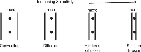
For large pores the transport process involves more bulk flow and convection, the microfiltration case. The rate of flow is assumed to be proportional to the pressure gradient, which is referred to as Darcy’s law. This states
Here Qt is the volumetric flux (velcoity), Pw is a parameter called the Darcy permeability, and ΔP is the applied pressure difference across a membrane and t is the thickness of the membrane. The Darcy permeability is modeled as based on laminar flow theory, where dp is the pore diameter for a single straight pore. A correction of ∊/τ is applied in general to account for the fact that the filter media does not have uniform straight pores. For simultaneous transport of two solutes there is hardly much difference in the rates, leading to no selectivity, as both solutes are carried by the flow.
For smaller pores transport is controlled by diffusion. If now the solute size is comparable to pore size the solute transport is restricted, leading to hindered diffusion. Selectivity is now achieved due to exclusion of larger solutes by a diffusion barrier. This is the situation prevailing in ultrafiltration; the membrane consists of meso- and micropores here.
Finally, if the pores are in the nanoscale range, the species dissolves in the membrane and then diffuses across the membrane. A high selectivity can be obtained due to exclusion casued by solubility differences. Often only one type of solute may be transported and the other species may be excluded; such membranes are normally referred to as semi-permeable. The osmotic pressure differences are created by the exclusion of one of the components in the liquid mixture, which is discussed in the following section. The driving force for transport has to be modified to include this factor.
Modeling of microfiltration and ultrafiltration can be done using concepts from flow in porous media, while nanofiltration and reverse osmosis requires the additional concept of osmotic pressure and its influence on the rate of transport. The transport mechanisms depend on the relative magnitude of solute size to pore size. Certain membranes can exclude solutes completely; such membranes are called semi-permeable. The pressure difference minus the osmotic pressure is then used as the driving force for solvent transport, as discussed in the next section.
28.2 Transport in Semi-Permeable Membranes
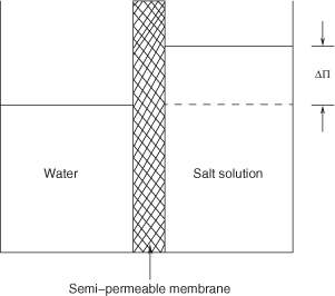
A semi-permeable membrane is a membrane that permits transport of only one species, usually a solvent such as water. A basic concept in understanding transport in membranes is the osmotic pressure for semi-permeable membranes. Consider a semi-permeable membrane that allows the solvent (water) to diffuse but not the solute (salt). Assume that these (pure water and a salt solution) are separated by a membrane into two compartments. At equilibrium there is a pressure difference between the solution and solvent, as shown in Figure 28.2. This pressure difference is called osmotic pressure and can be calculated based on either thermodynamic or kinetic considerations based on the concept of dynamic equilibrium.
28.2.1 Osmotic Pressure
An expression relating osmotic pressure to the solute concentration is derived in the following paragraphs. This is the minimum pressure that needs to be applied on the salt side in order to prevent an influx of water (solvent) to the salt side of the semi-permeable membrane.
At equilibrium the chemical potential of the solvent is the same on both sides of the membrane. On one side we have pure solvent and let represent its chemical potential (the subscript w is used since the solvent is very often water). On the other (salt solution) side, the chemical potential of water is related to its concentration and can be represented as
Here the second term on the right-hand side is correction due to concentration while the third term is the effect of pressure on the chemical potential. The pressure difference is pressure on the solution side minus that on the pure water side. From thermodynamic, we have
where is the partial molar volume of water. At equilibrium the chemical potential of water on the solution side μw is the same as the chemical potential of pure water:
Hence from Equation 28.2 we can find an expression for the difference in pressure across the membrane:
This pressure difference is often represented by ΔII, the usual notation for osmotic pressure. Also for dilute solutions we have
ln aw = ln xw = ln(1 – xs) ≈ –xs
where xs, the mole fraction of the solute. Hence Equation 28.4 can be written as
where is the concentration of the solute. This equation, known as the vant Hoff equation, has a resemblance to the ideal gas law. Note that the osmotic pressure is a colligative property, which is defined as any property that depends only on the concentration of the solute and not on the nature of the solute. Correction factors are applied to the previous equation for non-ideal solutions. Also, for solutes such as NaCl, a correction factor of two is used since NaCl exists as Na+ and Cl– ions in solutions.
28.2.2 Reverse Osmosis
Now, depending on the applied pressure difference compared to the osmotic pressure difference, three situations can arise, as presented in Figure 28.3.
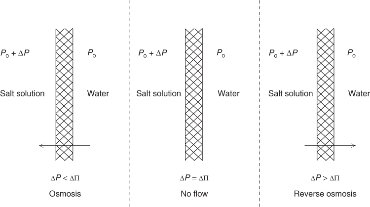
Figure 28.3 Illustration of influence of pressure difference across a semi-permeable membrane: osmosis, no flow, and reverse osmosis.
If ΔP < ΔII, there is osmotic flow with the solvent crossing (from the purer side) into the solute side. If the two are equal, we have a situation of equilibrium and there is no net flow across the membrane. The third case is when ΔP > ΔII, which is the condition for reverse osmosis. Here the solvent flows across the membrane (from the solute side) leaving behind an enriched solute solution and pure water as the permeate. This is the condition, for example, for desalination of sea water. The difference ΔP – ΔII may be considered the driving force for this case and the flux of the solvent, Jw, is represented as
This is a widely used equation for transport in osmosis and reverse osmosis. Here Kw is a permeability constant for the membrane in units of mole/m2Pa.s.
Partial Solute Rejection
The previous equation for the water flux is applicable under conditions of complete solute rejection. Normally there is some solute diffusion as well, that, complete solute rejection is not achieved. In such cases the flux expression is modified to
where σ is a factor between 0 and 1. This equation is referred to as the Starling equation in the semi-permeable membrane literature. The case of complete solute rejection corresponds to σ = 1 and the full impact of the osmotic pressure is left on the rate of transport. The other extreme is σ = 0, which is the case where the solute is also fully permeable. The parameter σ is known as the Staverman (1952) constant or simply the osmotic reflection coefficient.
For the case where the Staverman constant is not equal to one, an additional equation for the rate of solute transport (across the membrane) is needed. This is modeled by the following equation for the local combined flux:
The first term is the Fick’s law diffusion term for the solute while the second term is the solute carried with the solvent flow. xs is the salt mole fraction. A similar model for partial solute transport is the Kedem-Katchlski model discussed in Section 28.2.4.
We now consider a case with no solute transport (σ = 1) and show that the solute concentration is larger at the membrane surface compared to bulk liquid.
28.2.3 Concentration Polarization Effects
The convective flow of the solvent causes a corresponding solute flow on the liquid side of the membrane. However, the solute is not transported across the membrane (assuming complete rejection). This causes an increased solute concentration near the membrane surface compared to the bulk liquid. This phenomena is known as concentration polarization, and is illustrated in Figure 28.4.
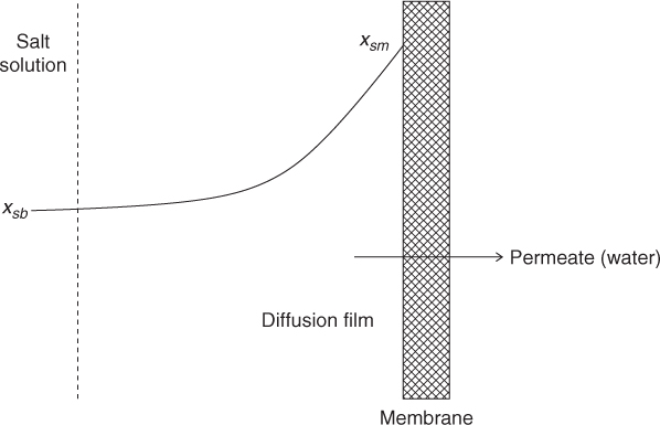
Figure 28.4 Illustration of concentration polarization effect. z is measured from right to left with z = 0 at the membrane surface.
The effect of concentration polarization is to increase the osmotic pressure at the surface of the membrane and thereby reduce the rate of solvent transport across the membrane. The effect can be modeled as follows by setting the net flux of the solute equal to zero. The solute transport (in the liquid film near the membrane surface) is the combination of diffusive and convective transport given by Equation 28.8. For the case where there is no solute transport, Js is set as zero. Hence the solute mole fraction in the film is given by the following equation:
The term on the left-hand side is the diffusive transport from the membrane to the bulk liquid. This is counterbalanced by the convective transport caused by the solvent flow, which is represented as the term on the right-hand side.
The boundary conditions are xsm at z = 0 and xsb at z = δ , where δ is the film thickness near the membrane surface. Integrating Equation 28.9 across the film we get
Integrating and taking the exponential on both sides gives an expression for the concentration polarization:
The osmotic pressure for solvent transport should therefore be based on xsm rather than xsb. If Δπ is the osmotic pressure based on bulk, then the effective osmotic pressure is
The exponential term is the correction factor for polarization. The transport equation for the solvent given by Equation 28.6 should be modified by multiplying the osmotic pressure by the correction factor. The modified equation (for the case of complete solute rejection) now reads
This is a transcendental equation for Jw and can be solved by iteration.
Simplified Form
For small values of JWδ/CD Equation 28.12 can be simplified by expanding the exponential term and keeping only the linear term. The resulting equation can be explicitly solved for Jw. The final answer shown here has a rather interesting physical meaning:
The denominator term on the right-hand side can be viewed as a sum of two resistances. The reciprocal of this quantity can be viewed as the measured effective permeability:
This effective permeability will be a function of flow rate and other parameters (due to the film thickness term) and hence will not be a true measure of the membrane permeability. This is again another effect where the mass transfer effect masks the true parameter value, similar to diffusion in a porous catalyst where the measured kinetic constant k is not necessarily the true kinetic constant k.
Returning back to partial solute transport (which applies if σ is less than one) we present next another model for membrane transport.
28.2.4 Kedem-Katchalski Model
The Kedem-Katchalski model is applicable when solute rejection is not complete. It attempts to provide a simplified representation based on the concept of irreversible thermodynamics and the Onsager reciprocal relations to simplify the number of model parameters. The model also finds important applications in transport in biological membranes.
The model provides the equations for solvent and solute flux across the membranes. A detailed derivation is presented in the original papers by Kedem and Katchalski (1958, 1961) and is not discussed here. A review paper by Jarzynska and Pietruszka (2008) gives the derivation in detail as well and provides details on the interpretation of the model parameters. The final equations of Kedem-Katchalsky model are summarized in the following.
The volumetric flux across the membrane is given as
The parameter σ is the solute rejection parameter introduced earlier. σ = 0 means complete accessibility for the solute transport while σ = 1 means complete rejection. Usually volumetric flux is commonly used; thus Qt is in m3/m2 s and Pw is a permeance (often referred to as permeability in the osmosis literature) and has units of m/s.Pa.
The solute transport rate is modeled as
where Cs,l.m is the log mean average of the solute concentration on either side of the membrane.
In this version of the Kedem-Katchalski model the three parameters are Pw, σ, and κ. The significance of these parameters is as follows: Pw is a measure of the Darcy permeability; σ is a measure of osmotic permeability (also called the reflection constant); and κ is a measure of diffusion of the solute in relation to convection.
Estimate of Transport Parameters
The parameters of the Kedem-Katchalsky model were related to fundamental transport parameters in Nakao and Kimura (1982) and Deen (1987). Pw is the Darcy permeability and is related to flow in a cylindrical pore of radius rp:
where t is the thickness of the membrane. This applies to the case where there are uniform straight pores. Such membranes are called track-etched membranes. Otherwise a tortuousity factor is added in the denominator.
The parameter σ is related to the ratio of the solute to the pore diameter, denoted as q:
Here SF is defined as
SF = (1 – q)2 – (1 – q)4
Finally κ is related to the diffusion coefficient of the solute in the pores:
Here SD is the correction factor for hindered diffusion:
SD = (1 – q)2
28.2.5 Equipment-Level Model
The local model for solvent and solute transport can be incorporated into a mesoscopic model to find the performance of a reverse osmosis unit or to design this equipment. The model is simple if the solute rejection is complete. Usually a plug flow is assumed for the feed side but the discretized form of this leads to a stagewise model similar to the gas permeator design model in Chapter 27. Either type of approach can be used, but stagewise calculation leads to algebraic equations and is simpler. The calculation procedure follows.
The pressure in each stage has to be calculated from a fluid dynamic equation. The pressure on the permeate side is usually fixed and the pressure drop is small on this side. The pressure difference is therefore calculated. The osmotic pressure value has to be adjusted at each stage corresponding to the salt concentration at that stage. ΔP – ΔII, the driving force at each stage, is calculated. Equation 28.13 can then be used to find the water flux across the membrane.
The material balance for water and salt on the feed side for this stage is now used to calculate the exit conditions of the stage. Calculations are repeated for the next stage until the end of the membrane unit is reached or the prescribed exit solute concentration is reached. Hence the analysis is similar to that for the gas permeator shown in Section 27.3.5. Further details are left as an exercise.
28.3 Forward Osmosis
Forward osmosis is an osmotic process that uses a semi-permeable membrane to effect separation of water from dissolved solutes. The driving force for this separation is an osmotic pressure gradient between a solution of high concentration, (often referred to as the draw solution) and a solution of lower concentration, referred to as the feed. The osmotic pressure gradient is used to induce a net flow of water through the membrane from the feed into the draw, thus effectively concentrating the feed.
The draw solution can consist of a single or multiple simple salts or can be a substance specifically tailored for forward osmosis applications. The feed solution can be a dilute product stream, a waste stream, or seawater. A schematic of a forward osmosis process is presented in Figure 28.5.
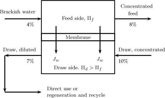
Figure 28.5 Schematic flowsheet for forward osmosis process. Solute % shown are for illustration only.
In this sketch a “dirty” stream of brackish water is used as a feed. The draw solution pulls water out of it. For example if the draw solution is concentrated fruit juice, it gets diluted and can be used for drinking purposes. Note that the water is drawn from a dirty source but is in potable form when permeated into the draw solution. This has applications in the food and beverage industry.
In some cases, the draw solution can be regenerated to remove salt (freezing or crystallization) and provide clean water. The draw solution can also be fed to a reverse osmosis system. The advantage (over direct reverse osmosis of the feed stream) is that a relatively clean stream is now fed to the reverse osmosis so that membrane fouling is reduced. Thus there are many applications of the forward osmosis processes. More details are available in Cath et al. (2006) together with illustrative applications.
28.4 Pervaporation
Pervaporation refers to removal of the permeate as vapor and represents an intermediate case between purely gas transport and purely liquid transport in a membrane. The component diffusing through the membrane changes its state from liquid to vapor while it is being transported across the membrane.
This requires vacuum equipment on the permeate side and can be costly. However in many cases the overall energy requirement is small compared to distillation and hence it can be an economical alternative, especially for separation of azeotropic mixtures. Composite membranes are used with the dense layer in contact with the liquid and the porous support layer exposed to vapor.
28.4.1 Illustrative Applications
There are a number of applications of pervaporation in practice; two are cited here:
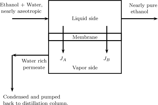
Separation of ethanol–water mixture: This is a hybrid process designed to produce 99.5% ethanol. A direct distillation cannot be used since an azeotrope is formed. Hence the overhead from the distillation, which has nearly 95% by weight of ethanol, is sent to pervaporation unit. The permeate is rich in water with 25% weight alcohol and is recycled back to the distillation column. The retentate is rich in alcohol and is the required product with 99.5% ethanol. The pervaporation membrane is a hydrophilic material and is selective to water transport. A schematic of this process is shown in Figure 28.6.
Separation of a volatile organic compound (VOC) from an aqueous solution. Here a hollow fiber module with silicone rubber is used. This permits the selective separation of the VOC. The retentate is almost pure water with less than 5 ppb of VOC. The permeate after condensation separates into two phases: (i) a nearly VOC-rich liquid and (ii) a water-rich liquid that is recycled back to the membrane unit. A schematic flow-sheet for this is showm in Figure 28.7.

The choice of membrane is critical depending on the application. The membrane can be either hydrophilic or hydrophobic. For water separation, the membrane used is hydrophilic, for example, PVA; water is the main permeate here. Hydrophobic membranes (e.g., silicone rubber, teflon, etc.) are preferred when the organic is the main permeating species, for example, VOC removal.
28.4.2 Model for Permeate Flux
Permeate flux is often modeled by the equation developed by Wijmans and Baker (1993). The fugacity difference is used as the driving force. This concept leads to the following equation for transport across a pervaporation membrane:
A similar equation holds for JB:
It is often difficult to predict the permeance parameters A and B from first principles. Hence this equation is often used to fit these parameters and to compare various PV membrane a rather than as the fundamental law.
The permeance can be a strong function of the feed composition. The temperature variation in the membrane is another complicating factor. A phase change occurs in the membrane and the heat of vaporization is provided by the cooling of the liquid as it permeates the dense layer. This decrease in temperature lowers the permeability and limits the extent of separation that can be achieved in a single unit. The second factor is the concentration dependency of the diffusion coefficient, primarily due to swelling. This increases the diffusion coefficient of both species and thereby alters the selectivity of one species over the other.
28.4.3 Local Permeate Composition
The local permeate composition for a given xA is related to the ratio of the flux of A, JA, to the total flux, JA + JB:
The flux expressions are given in Section 28.4.2 and can be combined and a quadratic similar to that for the gas permeation case can be derived. A modified pressure ratio parameter and a modified selectivity parameter are defined as follows:
The modified pressure ratio parameters for A and B are defined as
and
The modified selectivity parameter is
With these definitions, the expressions for the fluxes can be rearranged as
If these fluxes are substituted into the equation for the local mole fraction of in the permeate side (Equation 28.21) the following nonlinear equation (a quadratic) is obtained:
The local mole fraction is also equal to the local permeate mole fraction if there are no additional flows into or out of a local permeate control volume, for example, if the permeate is withdrawn locally and removed. In such cases, y′ is the composition of the vapor corresponding to x.
As an example, for 90% by weight of ethanol the local mole fraction of alcohol is 10% for a permeate pressure of 30 mm Hg. The permeate is richer in water. The permeate compositions for various liquid mole fractions of alcohol can be calculated in a similar manner and are shown in Figure 28.8. The membrane used was polyvinyl alcohol and it is observed that the permeate is richer in water than the liquid in contrast to distillation. Note also that the membrane is most selective in the range of alcohol mole per cent between 20 and 85 mole s.
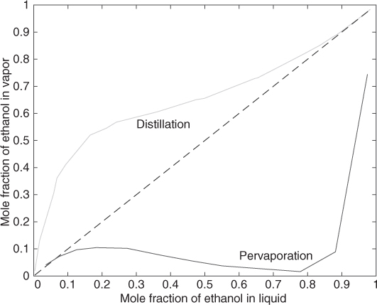
Figure 28.8 Permeate composition for pervaporation with a PVA membrane for an ethanol–water system at 60 °C.
A detailed dynamic model for pervaporation has been proposed by Bausa and Marquardt (2000).
Summary
Semi-permeable membranes used in many liquid phase separations permit the selective transport of only the solvent. Such membranes find application, for example, in water desalination. At low pressure differences, the water flows from the solvent to the salt side; this is osmosis. At a critical pressure difference equal to the osmotic pressure, the system is at equilibrium and no transport of water occurs in either direction. If the applied pressure is larger than the osmotic pressure then we have conditions for desalination (reverse osmosis; water flows out from the salt solution).
The rate of transport in a semi-permeable membrane is proportional to the difference between the applied pressure gradient and the osmotic pressure of the solution. The transport equation is given by the Starling equation (Equation 28.7) with a σ parameter known as the Staverman constant, which has a value of one for a completely semi-permeable case. σ = 0 applies when both the solute and solvent are equally permeable. Thus the Starling equation can be used for both a semi-permeable and completely permeable membrane with the appropriate choice of the σ parameter.
The solvent flow causes convection effects towards the membrane surface and there is a transport of solute (salt) by convection towards the membrane surface. Assuming there is no net transport of salt across the semi-permeable membrane, the concentration of the salt at the membrane surface has to assume a higher value compared to the bulk liquid value. This is required for the resulting diffusion flux to cancel out the convection flux. The phenomena is known as concentration polarization.
The effect of concentration polarization is to increase the osmotic pressure locally at the surface (due to higher salt concentration at the surface) thereby reducing the driving force for salt transport. The equation for solvent transport is now given by Equation 28.13. Note that the measured permeability under strong concentration polarization conditions is not the true membrane permeability.
The Kedem-Katchalsky model is an improvement over the Starling model and provides equations for both solvent and solute transport. The model is based on the concepts from irreversible thermodynamics and involves three parameters: Darcy permeability, osmotic permeability, and a diffusion parameter of the solute in relation to convection.
Forward osmosis is a process where water is drawn into a draw solution. The draw solution should have a higher solute concentration than the feed solution and the process of water transport is driven by osmotic pressure.
Pervaporation is a process where a vacuum is applied on the permeate side of a membrane and a vapor is drawn as the product. The retentate side is a liquid. Part of the membrane may be dry and part may be wet depending on the pressure profile in the membrane and the corresponding vapor–liquid equilibrium relationship.
The simplest model for pervaporation is to use the fugacity difference across the membrane as the driving force. However, the permeance is a strongly concentration-dependent parameter and depends on other factors such as swelling and temperature gradient across the membrane. Preliminary calculations can be done using the fugacity difference model to find the permeate composition.
Review Questions
28.1 What is ultrafiltration?
28.2 What is nanofiltration?
28.3 State Darcy’s law.
28.4 What is osmotic pressure?
28.5 How does the osmotic pressure depend on the solute concentration?
28.6 We have a 1 M NaCl and a 1 M KCl solution. Which one has larger osmotic pressure?
28.7 State the Starling equation for solvent transport.
28.8 What is the Staverman constant?
28.9 What is reverse osmosis?
28.10 State the Kedem-Katchalsky model.
28.11 What is meant by concentration polarization?
28.12 What is the effect of concentration polarization on the rate of transport across a reverse osmosis membrane?
28.13 What is forward osmosis?
28.14 What is pervaporation?
28.15 When is a hydrophilic membrane used in pervaporation?
28.16 When is a hydrophobic membrane used in pervaporation?
28.17 What is the commonly used driving force for transport in a pervaporation membrane?
28.18 Given x, the local mole fraction on the feed side, how would you calculate y, the mole fraction on the permeate side?
Problems
28.1 Minimum energy for separation. From thermodynamic relations for the chemical potential, calculate the minimum energy required to produce 1 mole of pure water from sea water by reverse osmosis at 300 K. Seawater has an NaCl salt concentration of 35.34 g/1000 g water and has a density of 1025 kg/m3.
28.2 Osmotic pressure and freezing point depression. The freezing point of a salt solution is less than that of water. Derive a relationship between osmotic pressure exerted by a solute and the freezing point depression caused by the solute in the solution. State the principle of thermodynamics that is common between the two phenomena.
28.3 Osmotic pressure and boiling point elevation. What is the boiling point of 1 M NaCl solution compared to pure water? The total pressure is 1 atm. State the principle of thermodynamics responsible for this elevation. Explain the relation of osmotic pressure to boiling point elevation
28.4 Water flux for various pressure gradients. A semi-permeable membrane has a Darcy permeability of 2.67 × 10⁻⁸ mol/cm2 s atm. The applied pressure difference is 10 atm on side A and 1 atm on side B. Find the water flux and direction of water flow for the following 3 cases where side B is maintained at different NaCl concentrations: side B is at 0, 0.1 M and 0.2 M NaCl concentration.
28.5 Effect of concentration polarization. At a certain point in a reverse osmosis module, the salt concentration is 1.8% by weight of NaCl and the applied pressure is 6.5 atm. On the permeate side the pressure is 2 atm. The permeance of the membrane is 1.1 × 10⁻⁵ g/cm2 s atm and there is complete solute rejection. Find the flux of water across the system. Neglect concentration polarization effects. If the mass transfer coefficient in the film near the membrane surface is 0.0025 cm/s, find the salt concentration at the membrane surface and find the reduction in water flux due to concentration polarization effects.
28.6 Correction for concentration polarization. A 1 M salt solution is maintained at a pressure of 10 atm above its osmotic pressure and a permeability of 1.5 × 10⁻⁵ g/cm2 s atm is reported based on the measured flux. Find the true permeability if the mass transfer coefficient is 0.0025 cm/s in the film near the membrane surface.
28.7 Design of a desalination unit. A salt solution with 3000 ppm of salt at a flow rate of 350 m3/day is to be desalinated. The feed-side pressure is 80 atm and the permeate pressure is 2 atm. The permeance is 1.1 × 10⁻⁵ g/cm2 s atm and the external mass transfer coefficient is 0.005 cm/s. Design a reverse osmosis system for a 50% recovery of potable water.
28.8 Transport rate in a inorganic membrane. The transport of various solutes in inorganic nanofilration membranes was studied by Tsuru et a. (2000) and the following data was given for σ and κ:
Species |
σ |
κ |
Methanol |
0.35 |
4.58 |
Ethanol |
0.55 |
4.23 |
Butanol |
0.85 |
1.58 |
Estimate the fraction of solute rejected for each of these cases.
28.9 Estimation of parameters in the Kedem-Katchalski model. The Stokes radius of methanol is estimated as 0.137 nm. Find the σ parameter for a membrane with a pore radius of 1 nm. Find the κ parameter if the diffusion coefficient is 1.79 × 10⁻⁹ m2/s. Assume a porosity of 0.5. The Darcy permeability coefficient for water is 3 m/s Pa.
28.10 Area calculation for concentration of fruit juice. Fruit juice is to be concentrated from an initial concentration of 10% to 35%. The operating pressure is 40 atm, which is equivalent to the osmotic pressure of a 42% solution. The permeability is 2 × 10⁻⁶ m3/m2 min atm. Find the surface area of the membrane needed to achieve the required concentration.
28.11 Flux and area calculation in forward osmosis. For the concentrations shown in Figure 28.5, find the membrane area to be used if the water permeability of the membrane is 5 L/m2 hour bar.
28.12 Pervaporation permeabilty from measured data. A pervaporation membrane was exposed to 90% ethanol and the rest water a 60° C and the flux of alcohol was measured as 0.29 kg/m2 hour. The permeate composition was 7.1% alcohol. The liquid side was at atmospheric pressure while the gas side was at 15 mm Hg. Find the permeability and the selectivity of the membrane for water. Use the Margules equation for the calculation of the activity coefficients (W = water, A = alcohol):
28.13 Separation calculation for pervaporation. A membrane used for alcohol–water separation has a permeance of 152 mol/m2 hour atm for water and a selectivity of 175. Calculate the local permeate composition for 90% alcohol in the feed and a pressure on the vapor side of 30 mm Hg.
28.14 Permeate composition. Calculate the local permeate mole fraction for 90% by mass of alcohol over a membrane operated at 30 mm Hg downstream pressure. Use the Margules equation for activity coefficients. Use the following data for the membrane: permeance for water = 152 mol/m2 hour atm; permeance for alcohol = 0.87 mol/m2 hour atm; vapor pressure of water = 148 mm Hg; vapor pressure of alcohol = 340 mm Hg.
28.15 Effect of feed composition and downstream pressure. Calculate the permeate composition of the previous problem for alcohol mass percents of 95%, 99%, and 99.9%. The following results are shown in McCabe et al. (2010). Verify these results.
% alcohol by mass |
xW |
yw |
95 |
0.1186 |
0.915 |
99 |
0.0252 |
0.256 |
99.9 |
0.00255 |
0.026 |
Repeat the calculations of the above problem for a downstream pressure of 15 mm Hg. The results show how the permeate gets relatively richer in alcohol as the alcohol mole fraction in the feed increases and therefore getting to almost pure alcohol gets progressively difficult.