5.1 Multi-Group CFA Model

The multi-group CFA model (Sörbom, 1974; Hayduk, 1987; Bollen, 1989a) is often used to test factorial invariance of measurement scales. According to Jöreskog (1971b), to test factorial invariance using multi-group CFA, one should first conduct an omnibus test of equality of the observed indicator variance/covariance matrix across groups. If the omnibus test demonstrates invariance of observed variances/covariances, then no more invariance tests are needed. However, the necessity of the global omnibus test is debatable, and there is no consensus in practice of multi-group CFA modeling in this regard. Studies have found some inconsistencies in the omnibus invariance test and model parameter invariance test. For example, even though the omnibus test results show invariance of the observed variances/covariances, some measurement parameters (e.g., factor loadings and item intercepts) and structural parameters (e.g., factor variances/covariances, and factor means) may be still noninvariant across groups, and vice versa (Byrne, 2006). We prefer not to conduct the omnibus test, but focus on tests of measurement invariance and structural invariance in this section.

Conceptually speaking, factorial invariance of a scale consists of two different kinds of invariance: measurement invariance and structural invariance. The former involves invariance of patterns of factor loadings, values of factor loadings, observed indicator/item intercepts, and error variances; and the latter includes invariance of factor variances/covariances and factor means. The measurement invariance is usually tested first, and then structural invariance because establishment of measurement invariance across groups is a logical prerequisite to conducting substantive cross-group comparisons (Vandenberg and Lance, 2000).

Testing measurement invariance is to ensure that the observed scale indicators/items under study measure the same theoretical constructs (latent variables or factors) in all groups. It is commonly known that measurement invariance is a prerequisite for group comparison. If measurement invariance does not hold, analyses of the corresponding measures do not produce meaningful results, and findings of differences between groups cannot be unambiguously interpreted (Horn and McArdle, 1992). In statistical tests, such as t-test, measurement invariance is usually assumed across the groups under comparison. For an unobserved construct/factor with multiple observed indicator variables/items, its measurement invariance can be tested using multi-group CFA models.

Measurement invariance involves four different levels: configural invariance, weak measurement invariance, strong measurement invariance, and strict measurement invariance (Meredith, 1993; Widaman and Reise, 1997). The different levels of measurement invariance are tested in several hierarchical steps.

Measurement invariance is a prerequisite to testing structural invariance. After measurement invariance (usually metric and scalar invariance) is demonstrated, we can proceed to test structural invariance by testing invariance of structural parameters, such as factor variance, covariance, and factor means across groups. Given measurement invariance, structural invariance will provide useful information about the differences in the theoretical constructs across groups. Note that noninvariance of the structural parameters does not mean any problem with the instrument under study, but simply means population heterogeneity, regarding the corresponding parameters. Researchers expect the measuring instrument to operate equivalently across different populations/groups so that the same theoretical constructs could be measured in the same way in different populations/groups. However, there is no reason to expect that the levels of the constructs/latent variables under study or the relationships among the latent variables remain unchanged among different populations or groups. It is logical to ensure measurement invariance across populations/groups, and then test structure invariance or compare structural parameters across populations/groups; otherwise, we may not know whether we are comparing like with unlike or not. The steps of testing structural invariance are described as the follows:

1. Test invariance of factor variance. The variance of a factor is a measure of variation or dispersion of the factor scores. Usually, invariance of factor variance is not of typical interest to researchers. In testing structural invariance, people are more interested in testing invariance of factor covariance and invariance of factor means. However, when one is interested in testing invariance of item reliabilities, invariance of factor variance must be ensured because it is considered a precondition to testing invariance of item reliabilities (Vandenberg and Lance, 2000).

2. Test invariance of factor covariance. A covariance between two factors represents the association between the two factors. When factor variance invariance holds, factor covariance invariance is equivalent to factor correlation invariance across groups. Researchers are often interested in testing factor covariance invariance because it would be useful to know whether the relationships between factors under study remain unchanged in different populations.

Both factor variance and covariance invariance can also be tested simultaneously. If both factor variances and covariances are invariant across groups, we conclude that both dispersion of factor scores and the relationships between factors are invariant across groups. In addition, such a test can also be considered as an omnibus test for possible higher order factorial invariance. For example, in the second-order CFA model discussed in Chapter 2, testing the first-order factor variance and covariance invariance can be considered as an omnibus test for factorial structure of the second-order part of the model. However, just like the omnibus test for the first-order CFA model, even if the omnibus test results demonstrate invariance of the first-order factor variance/covariance, the second-order measurement parameters (e.g., second-order factor loadings and the first-order factor intercepts) and structural parameters (e.g., second-order factor variances/covariances, and second-order factor means) may still be noninvariant across groups and vice versa.

3. Test factor mean invariance. An important aspect of multi-group CFA modeling is to test factor mean differences between groups. Since factor means cannot be identified in all the groups, multi-group CFA does not estimate the absolute values of factor means for each group. Instead, one of the groups must be treated as the reference group, and then differences in factor means between other groups (comparison groups) and the reference group are estimated (Byrne, 2001, 2006; Bentler, 2005). This is done by fixing all the factor means to 0s in the reference group, and estimate the factor means as free parameters in other groups. The estimated factor means in each comparison group are in fact the difference in the factor mean between this group and the reference group. It should be kept in mind when testing factor mean invariance or comparing factor means across groups, factor loadings and indicator/item intercepts must be invariant across groups; that is, the observed item scores from different groups must have the same measurement metric and the same scalar in order to compare factor means across groups.

Testing invariance of some measurement parameters (e.g., factor loadings and error variance) and some structural parameters (e.g., factor variances and covariances) could be conducted based on analysis of COVS, but testing invariance of indicator intercepts and factor means must be conducted based on analysis of MACS. As aforementioned, model estimations are based on analysis of MACS by default since Mplus version 5. All the models for invariance tests in this chapter are conducted based on analysis of MACS.

In the hierarchical steps of testing measurement invariance and structural invariance, different restrictions are imposed on various parameters of interest across groups. At each testing step, model χ² statistics between the restricted and unrestricted models are used to conduct the LR test for model comparison. If the model χ² statistic does not change significantly after imposing the restrictions, then the corresponding hypothesis of parameter invariance is retained. Recall that the model χ² statistic cannot be directly used for the LR test when robust estimators, such as MLM, MLR or WLSM, are used for model estimation; instead, a scaled difference in χ²s should be used (Chapter 2). For the purpose of simplicity, ML is used for model estimation in this chapter so that the model χ² statistic can be directly used for LR tests.

In addition, change in CFI () has been increasingly used to evaluate invariance in multi-group modeling. A less than or equal to 0.01 between nested models is considered as a criterion of invariance. A larger than 0.01 indicates a meaningful change in model fit for testing invariance (Cheung and Rensvold, 2002).

5.1.1 Multi-Group First-Order CFA

We start with testing factorial invariance in a first-order CFA model. The data used for modeling were two independent samples selected from the natural history studies on rural drug use practices in Ohio (n = 248) and Kentucky (n = 225) in the USA between 2003 and 2005 (Booth et al., 2006). Study eligibility included the following: (1) having provided informed consent to participate in the study; (2) being age 18 or older; (3) self-reported use of crack-cocaine, powdered cocaine, or methamphetamine/amphetamine in the past 30 days; (4) no recent formal substance abuse treatment (past 30 days); and (5) residence in one of the targeted counties. Respondent-driven sampling, which has been increasingly applied to recruit hidden drug user populations, was used for sample recruitment in the current project (Heckathorn, 1997, 2002). The project participants were followed up every 6 months after the baseline interview for three consecutive years. More detail on recruitment approaches and sampling method can be found in previous publications (Draus et al., 2005; Wang et al., 2007).

Again, the BSI-18 scale was used for model demonstration. The three dimensions of psychiatric disorders measured by the BSI-18 are: somatization (SOM), depression (DEP), and anxiety (ANX). Each of the three subscales was measured by six items, respectively (Table 2.1). All the BSI-18 items are measured on a five-point Likert scale (0, not at all; 1, a little bit; 2, moderately; 3, quite a bit; 4, extremely). All subscales of the BSI-18 have excellent reliabilities with Cronbach's alpha greater than 0.80 in the populations under study.

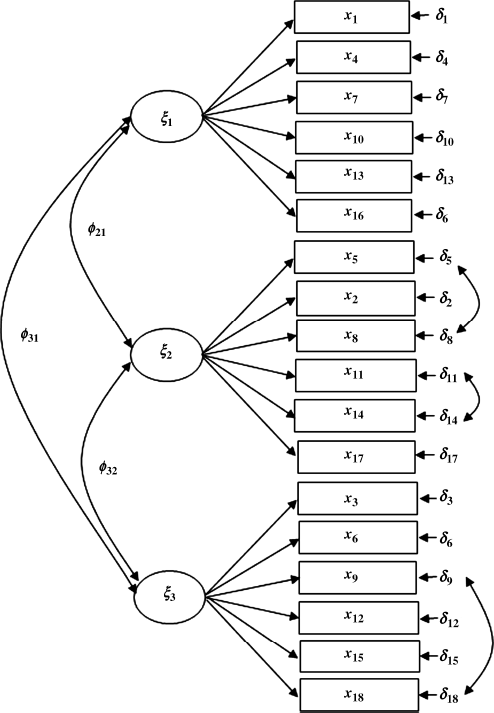
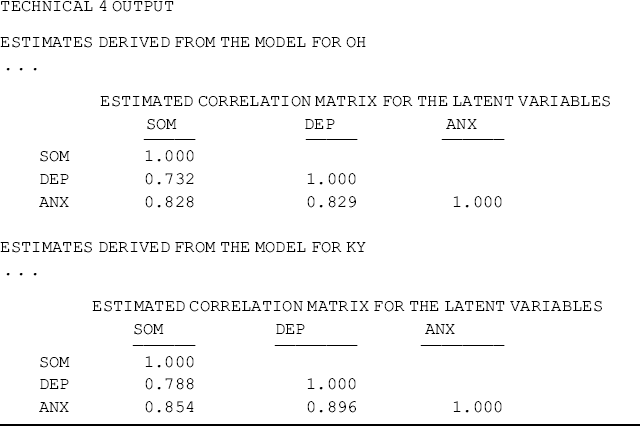
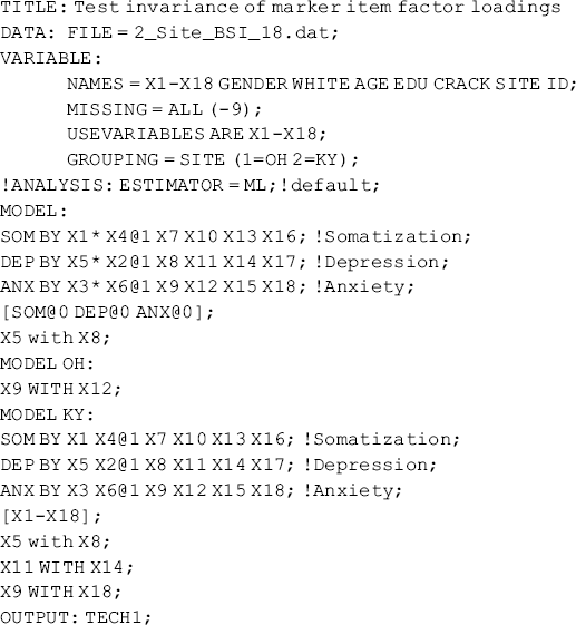
The baseline model: CFA models will be used to fit the Ohio and Kentucky samples separately, and the parsimonious and meaningful model that fits data well will be defined as the baseline model for each group (i.e., each of the two states in this example). Similar but not completely identical baseline models are identified and shown in Figures 5.1 and 5.2. The two baseline models have the same three factors (SOM, DEP, and ANX) with the same pattern of fixed and free factor loadings. However, to improve model fit, a couple of error covariances were specified in the models: two error covariances Cov () and Cov () were specified in the baseline model for the Ohio sample, and three error covariances Cov (), Cov (), and Cov () for the Kentucky sample. The baseline models of different groups that will be integrated in the configural model must be similar, but are not necessary to be completely identical (Byrne, Shavelson and Muthén, 1989; Bentler, 2005).

Figure 5.1 Baseline model: Ohio.

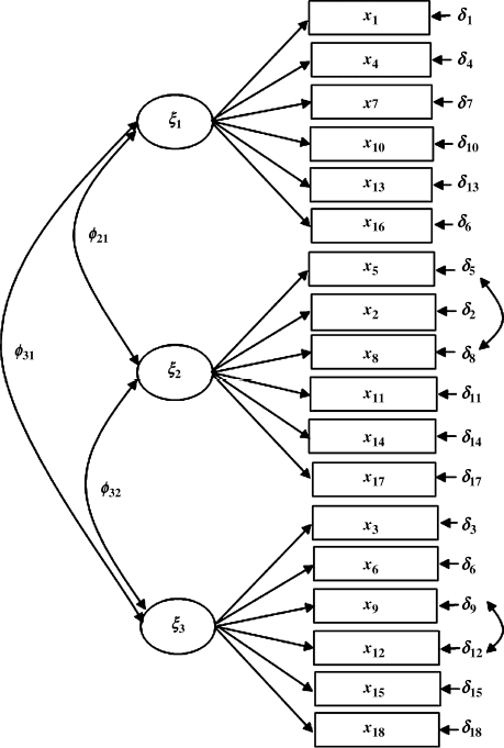
Figure 5.2 Baseline model: Kentucky.

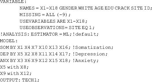
The Mplus programs for the baseline models follow:

Mplus Program 5.1

Mplus Program 5.2

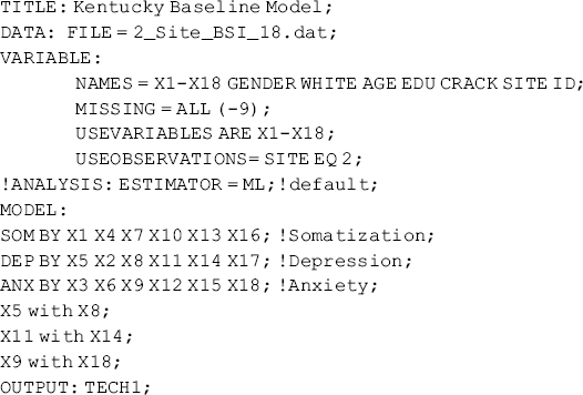
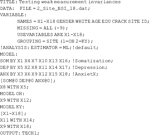
In the above Mplus programs, data are saved in text file 2_Site_BSI_18.dat, in which Ohio and Kentucky samples are appended together. In the VARIABLE command, the USEOBSERVATIONS option is used to select a specific sample for analysis. The indicator variable Site (1 = Ohio, 2 = Kentucky) identifies the samples/groups in the data. The default ML estimator is used for model estimation. Upon model fit indices from exploratory modeling, the statements of x5 with x8 and x9 with x12 in the MODEL command, are used to specify error covariances Cov () and Cov () in the Ohio model; while three error covariances [Cov (), Cov () and Cov ()] are specified in the Kentucky model, for the purpose of model fit improvement. All models are estimated based on analysis of MACS that is the default. For the purpose of model identification, factor means are all set to zero by default, while item intercepts are estimated. The model results are shown in Tables 5.1 and 5.2, respectively.

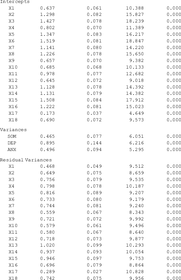
Table 5.1 Selected Mplus output: baseline models for Ohio.

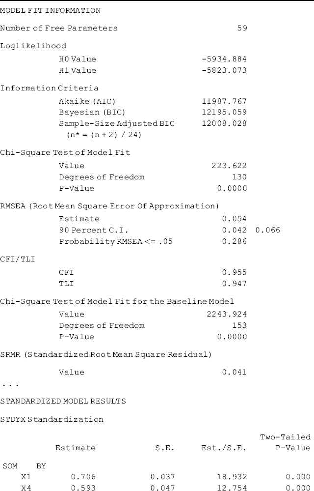
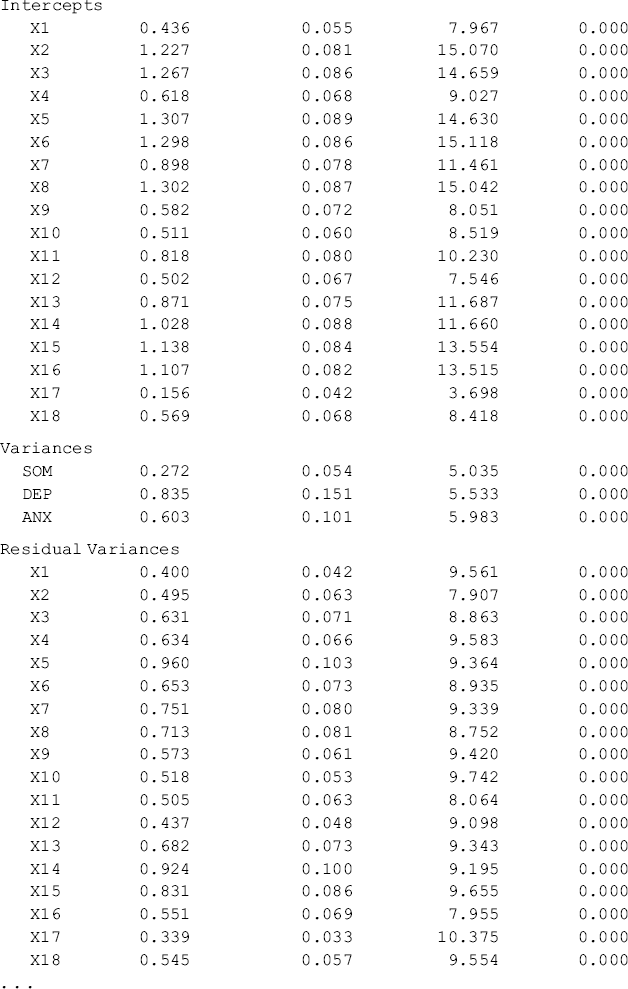
Table 5.2 Selected Mplus output: baseline models for Kentucky.

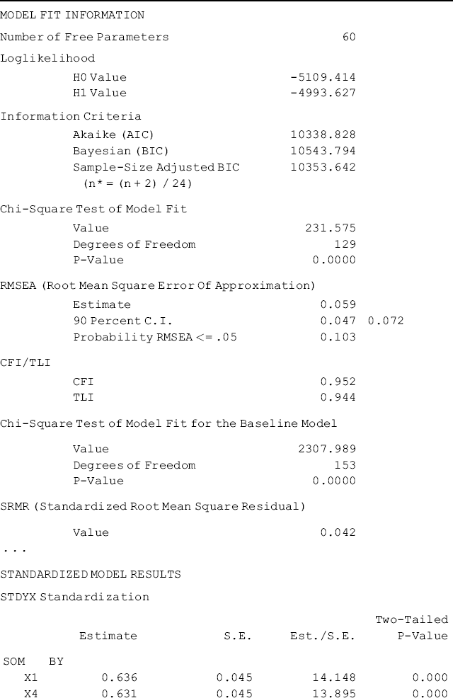
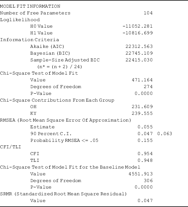
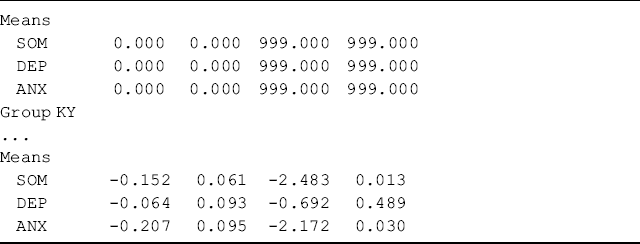
The results of the two baseline models show that the BSI-18 items are highly loaded to their underlying factors in the two samples, and both models fit data very well. The model fit indices for Ohio are: RMSEA = 0.054, 90% CI = (0.042, 0.066), close-fit test P-value = 0.286, CFI = 0.955, TLI = 0.947, and SRMR = 0.041. The corresponding model fit indices for Kentucky are: RMSEA = 0.059, 90% CI = (0.047, 0.072), close-fit test P-value = 0.103, CFI = 0.952, TLI = 0.944, and SRMR = 0.042 (Tables 5.1 and 5.2). The model results seemingly show that the BSI-18 measures the theoretically designed constructs very well in each of the populations under study (i.e., rural drug users in Ohio and Kentucky). However, configural invariance needs to be statistically tested in a configural model (Horn and McArdle, 1992; Reise, Widaman, and Pugh, 1993; Vandenberg and Lance, 2000; Byrne, 2006).

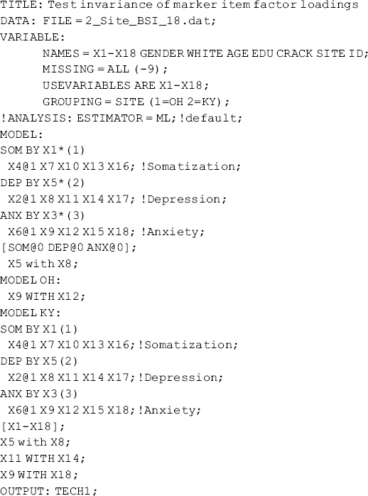
Testing configural invariance: After the baseline model has been determined for each sample, the two baseline models are combined into a multi-group model to form a configural model, in which the same number of factors and the same pattern of fixed and free factor loadings are specified in each of the groups, but no equality restrictions are imposed on any measurement and structural parameter across groups. And then the model is estimated simultaneously with all the groups. Only if the configural invariance is demonstrated across groups, can further invariance tests, such as metric invariance, scalar invariance, factor variance and covariance invariance, and factor mean invariance, be tested; otherwise, all other invariance tests are unwarranted. The configural model can be expressed as the following:

(5.1)

(5.2)

In Equation (5.1), covariance structure of the observed indicator variables are expressed as a function of factor loadings, factor variances/covariances, and error variances/covariances (Appendix 1.A). The same pattern of free and fixed factor is specified for each group,² but no equality restrictions are imposed on any of the model parameters. The superscript ‘g’ on matrix , and represents the elements of each matrix are noninvariant across groups. Equation (5.2) expresses the mean structure of the observed indicator variables, where the indicator means () are defined as a function of two types of unknown mean structure parameters: the item intercepts () and the factor means ().³ To estimate the mean structural parameters and , the available observed mean structure information (i.e., the observed indicator means) in our example is g × 18 = 2 × 18 = 36. However, the total number of parameters in and is 2 × 18 + 3 = 39. Thus, the mean structure part of the model is unidentified. To solve such a problem, a configural model is usually estimated using only the covariance structure (COVS) [i.e., Equation (5.1)]. If the MACS is analyzed (the default since Mplus version 5), some restrictions are needed in the mean structure part of the model. In order to make Equation (5.2) identifiable, we set the factor means () in the equation to 0. The Mplus program for the configural model follows.

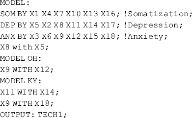
Mplus Program 5.3

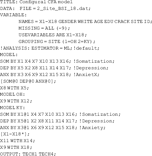
where both Ohio and Kentucky samples that are appended in data set 2_Site_BSI_18.dat are used for simultaneous analysis. The GROUPING statement in the VARIABLE command specifies grouping variables (i.e., SITE in this example) that contains the information about group membership.⁴ There are two kinds of MODEL commands in Mplus Program 5.3: the commands ‘MODEL’ and ‘MODEL’ followed by a label (e.g., OH and KY in this example). The former is the overall MODEL command that applies to all the groups under study. For example, the statement ‘X8 WITH X5’ in the overall MODEL command specifies the common error covariances Cov () in each group, but no equality restriction; and the statement [SOM@0 DEP@0 ANX@0] sets the means of three factors to zero in each group. The commands MODEL OH and MODEL KY are group-specific MODEL commands, in which specific models components that differ from the overall model are specified for specific groups. For example, error covariance Cov () is specified in the Ohio model, and error covariances Cov () and Cov () are specified in the Kentucky model.

By default, the overall MODEL command sets some measurement parameters, such as factor loading and intercepts of continuous outcome variables (or thresholds of categorical outcome variables) equal across groups, while letting all structural parameters (e.g., factor variances/covariances and factor means) be free parameters. To release equality constraints on factor loadings, the same pattern of factor loading is re-specified in group-specific MODEL KY command for the Kentucky sample, thus allowing factor loadings to vary across groups. In addition, the statement [X1-X18^∗] in the group-specific MODEL commands MODEL KY releases the equality restrictions on item intercepts imposed by default in the overall MODEL command.

The model is estimated using the default ML estimator where the fitting function represents a weighted combination of model fit across groups. As such, the model χ² difference of nested models will follow a χ² distribution, and the LR can be used for model comparisons. As aforementioned, when a robust estimator (e.g., MLR, MLM, WLSM) is used for model estimation, the conventional approach of the LR test is not appropriate because difference between two scaled χ²s for nested models does not follow χ² distribution. The appropriate approaches of conducting nested model comparisons are described and demonstrated in Chapter 2. To make model comparison easier, ML is used for model estimation in this section.

An important issue of testing factorial invariance using the multi-group CFA model is to ensure that each factor is on the common scale across groups; that is, the scales of each factor should be established by fixing factor loading of the same item in each group to 1.0. In our example, factor loading of the first item of each factor (i.e., indicator x₁ of factor SOM, x₅ of factor DEP, and x₃ of factor ANX) is set to 1.0 in each group. The factor loading of the first item of each factor in the BY statement of the overall MODEL command is fixed to 1.0 by default; however, no factor loadings are fixed by default in the BY statement in the group-specific MODEL commands. In Mplus Program 5.3, the factor loadings of x₁, x₅, and x₃ are fixed to 1.0 manually in the MODEL KY command.

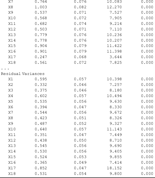
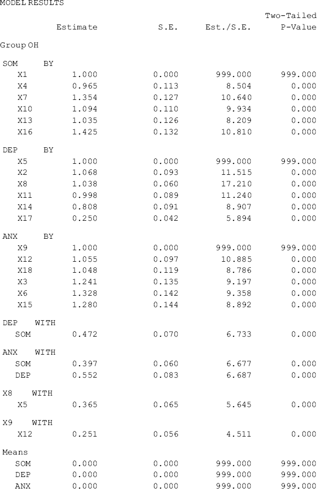
The results of the configural model are shown in Table 5.3, where separate sets of parameter are reported (e.g., factor loadings, item intercepts, residual variances, factor variances and covariances) for each group, but only one set of model fit statistics and indices (e.g., model χ² statistics, RMSEA, CFI, TLI, and SRMR) are reported.

Table 5.3 Selected Mplus output: configural CFA model.

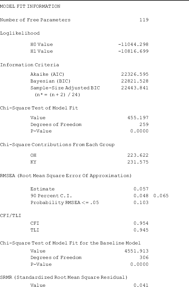
The model fits data very well: RMSEA = 0.057, 90% CI = (0.048, 0.065), close-fit test P-value = 0.103, CFI = 0.954, TLI = 0.945, and SRMR = 0.041. Note when ML estimator is used for model estimation, the model fit χ² statistic for the configural model equals the sum of the model χ² statistics of the two separate baseline models. In our example, the overall model fit χ² statistic, = 455.197 for the configural model, which equals the sum of the χ² statistics of the Ohio and Kentucky baseline models ( = 223.622 and = 231.575, respectively). When a robust estimator (e.g., MLR, MLM) is used, the χ² statistics of the separate baseline models would not be summing up to the χ² statistic of the configural model.

The configural model serves as a base for model comparisons in multi-group modeling. The model provides the baseline value against which subsequently specified restricted models will be compared. In the following we will examine factorial invariance of the BSI-18 by testing a hierarchical series of models. We will first test measurement invariance by conducting hierarchical tests for invariance of measurement parameters: weak measurement invariance, strong measurement invariance, and strict measurement invariance. Once measurement invariance is demonstrated, we will further test invariance of structural parameters, such as factor variance invariance, factor covariance invariance, and factor mean invariance.

Test weak measurement invariance: Weak measurement invariance is defined as invariance of factor loadings across groups as described in the following equations:

(5.3)

(5.4)

where the superscript ‘g’ is removed from the factor loading matrix () in both Equations (5.3) and (5.4), indicating the elements of this matrix are invariant across groups. The factor mean term () in Equation (5.4) is set to zero for the purpose of model identification, and the model is estimated based on analysis of MACS by default.

Invariance of factor loadings across groups is considered the minimal condition for measurement invariance. As such, testing for invariance of factor loadings typically is the first step in the measurement invariance test. Invariance of factor loadings indicates the metric of factor scores is invariant across groups or a unit change in the factor score would result in the same amount of change in the observed item score across groups. In contrast, absence of weak measurement invariance across groups indicates that the observed indicator variables measure different constructs/factors in different groups. Only if invariance of factor loadings has been demonstrated, relationships between factors and external variables can be compared across groups.

In our example model, the null hypothesis of testing metric invariance is: factor loadings are invariant across groups (i.e., factor loadings are not significantly different between the Ohio and Kentucky samples). To test such a hypothesis, the most frequently used approach is the LR test based on χ² difference between the restricted model (e.g., factor loadings are set equal across groups) and the unrestricted configural model. Model χ² difference between two nested models follows a χ² distribution with a df that is the difference in df between the two models being compared.

In addition, change in CFI () will also be used to evaluate invariance in multi-group modeling. A less than or equal to 0.01 between nested models indicates no significant difference between two nested models in regard to model fit (Cheung and Rensvold, 2002).

Note that in multi-group modeling, the standardized parameter estimates could still be noninvariant even if the unstandardized parameter estimates are invariant across groups because the variances of observed and latent variables are often different across groups. To achieve the parameter invariance in a standardized solution, Jöreskog and Sörbom (1989) developed a common metric completely standardized solution, which is available in LISREL. Unfortunately, the current version of Mplus does not provide such standardization for multi-group modeling. Therefore, testing for invariance of only unstandardized parameter estimates is considered in this chapter.

Mplus Program 5.4

Different from Mplus Program 5.3, factor loadings are not specified in the group-specific MODEL commands in Mplus Program 5.4; thus factor loadings are treated invariant across groups in Mplus by default. Selected model results are shown in Table 5.4.

Table 5.4 Selected Mplus output: multi-group CFA model with equality restrictions on factor loadings.

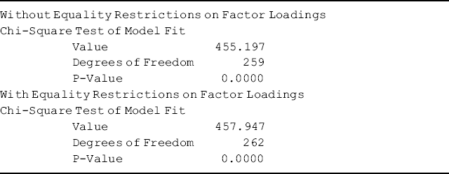
Since this model is nested in the configural model specified in Mplus Program 5.3, the LR test is used to test model difference. Change in model χ² statistic between the configural model and the current model follows a χ² distribution: = (471.164 − 455.197) = 15.967 with df of (274 − 259) = 15, which is not statistically significant (P = 0.3842). ⁵ In addition, there is no change in CFI. We, therefore, conclude that the null hypothesis of metric invariance cannot be rejected. Metric invariance or invariance of factor loadings means that the relationships between responses to the BSI-18 items and their underlying factors are not significantly different across groups. In other words, the latent variables are measured in the same way with the same metric in the two target populations.

If the hypothesis of factor loading invariance were rejected, it would imply that the instrument under study (e.g., BSI-18 in our example) is problematic because it may measure different constructs/factors in different populations; thus no further invariance test is necessary. It does not make sense to examine invariance of structural parameters (e.g., factor means and relationships between factors) when measures of factors differ across groups. However, when the full measurement invariance does not hold, some researchers suggest that partial measurement invariance may be tested, and comparisons of groups on latent variables can be conducted if partial measurement invariance holds (Byrne, Shavelson, and Muthén, 1989). One may also identify and delete the problematic items, and then retest the metric invariance hypothesis using a subset of the original items. However, these two approaches are debatable.

As discussed in Chapter 2, one of the factor loadings of each factor or the factor variance must be fixed (usually to 1.0) in a CFA model to define the scale of the factor; otherwise, the model will not be identified. These items are called ‘marker items.’ In Mplus Programs 5.3 and 5.4, the marker items are x₁, x₅, and x₃, whose factor loadings are not model estimated, but fixed; therefore, invariance of the marker items' factor loadings are not tested in the LR test. In order to have meaningful comparisons of structural parameters across groups, we need to ensure, instead of just assume, that the factor loadings of the marker items are also invariant across groups. The following Mplus programs are used to test invariance of the factor loadings of the marker items x₁, x₅, and x₃.

Mplus Program 5.5a

where factor loadings of another three items (i.e., x₄, x₂, and x₆) are fixed to 1.0 and all other factor loadings are set to be free parameters in each group. In Mplus Program 5.5b, equality restrictions will be imposed on the factor loadings of x₁, x₅, and x₃ across groups. And then, model statistics with and without the equality restrictions will be used to conduct a LR test for factor loading invariance of items x₁, x₅, and x₃.

Mplus Program 5.5b

To impose equality restrictions on the factor loadings of items x₁, x₅, and x₃ across groups, different numbers in parentheses are placed after the items in the BY statements of the overall MODEL command and in the group-specific MODEL KY command. Note that one restriction should be specified per line; otherwise, the program will not run. The difference in model statistics between the models with and without equality restriction (Table 5.5) follows a statistic of 2.75 with df = 3, which is not statistically significant (P = 0.4318), indicating that the factor loadings of the items x₁, x₅, and x₃ in our example model are invariant across groups. We, therefore, conclude that these three items are appropriate marker items for the example model.

Table 5.5 Model χ² statistics of multi-group CFA model with and without equality restrictions on factor loadings.

The model of testing factor loading invariance is the least restricted; next we will impose more restrictions in the model to further test measurement invariance of the BSI-18. In multi-group modeling, the tests for parameter invariance are in a hierarchical order and become increasingly restrictive. It is a common practice that once parameters are examined invariant across groups; equality restrictions on those parameters should remain in subsequent invariance tests.

Test strong measurement invariance: Strong measurement invariance is defined as both factor loadings and item intercepts are invariant across groups. The following equations describe the strong measurement invariance model:

(5.5)

(5.6)

where the superscript ‘g’ is removed from both the factor loading matrix and item intercept vector , indicating that the item measures have the same metric and scalar in all groups, while the error variances⁶ (the diagonal values of ) and the structural parameters still remain noninvariant across groups. Once the elements of are restricted to be invariant across groups, the free mean structure parameters in Equation (5.6) are 18 item intercepts plus 3 factor mean differences, which is smaller than the observed mean structure data points (i.e., 2 × 18 = 36), thus both item intercepts and group differences in factor means are identified in this equation. However, since testing for invariance of factor loadings and item intercepts is of interest here, we set factor means () to zeros in our example model. The Mplus program for testing the hypothesis of strong measurement invariance follows.

Mplus Program 5.6

The only difference between Mplus Program 5.6 and Mplus Program 5.4 is that the statement [X1-X18] is removed from the specific MODEL command for the Kentucky sample in Mplus Program 5.6. Since the measurement model is only specified in the overall MODEL command, by default Mplus sets both factor loadings and the item intercepts invariant across groups. As in Mplus Program 5.4, the statement [SOM@0 DEP@0 ANX@0] in the overall MODEL command sets all factor means to zero. Selected model results are shown in Table 5.6.

Table 5.6 Selected Mplus output: multi-group CFA model with equality restrictions on both factor loadings and item intercepts.

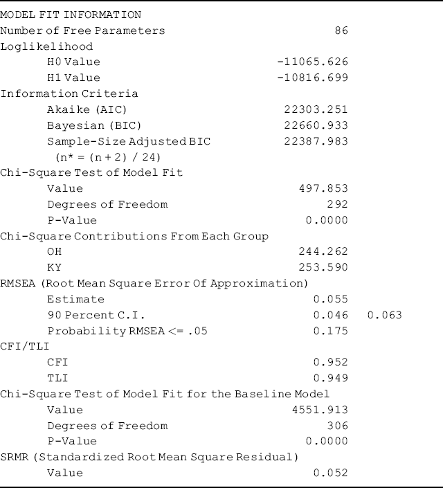
Since we are testing both factor loading invariance and item intercept invariance, we need to compare the current strong measurement invariance model with the configural model that does not impose any restrictions on the corresponding parameters. The LR test based on the model difference between the current model and the configural model shows = (497.853 − 455.197) = 42.656 with df = (292 − 259) = 33, which is not statistically significant (P = 0.1211). In addition, change in CFI, = (0.954 − 0.952) = 0.002, which is much smaller than 0.01. Thus, the null hypothesis of strong measurement invariance cannot be rejected. In other words, both factor loadings and item intercepts of the BSI-18 are invariant across groups.

Test strict measurement invariance: The last test of measurement invariance is to test error variance invariance. If factor loadings and item intercepts, as well as error variances, are all invariant across groups, strict measurement invariance is demonstrated. The strict measurement invariance model is expressed as follows:

(5.7)

(5.8)

where the superscript ‘g’ is removed from factor loading matrix (), item intercept vector (), and error variance matrix (). Equality restriction on error variance means that the amount of variance in each observed indicator that is not explained by its underlying factor(s) is invariant across groups. This implies that the group difference in variance of an observed indicator/item is only attributed to group difference in variance of its underlying factor ().

Again, the structural parameters are not of interest here, and factor means () are set to zeros although they are indentified in the mean structure equation.

Mplus Program 5.7

The only difference between Mplus Program 5.7 and Mplus Program 5.6 is that equality restrictions are imposed to not only on factor loadings and item intercepts, but also on the corresponding item variances across groups. Selected model results are shown in Table 5.7.

Table 5.7 Selected Mplus output: testing strict measurement invariance.

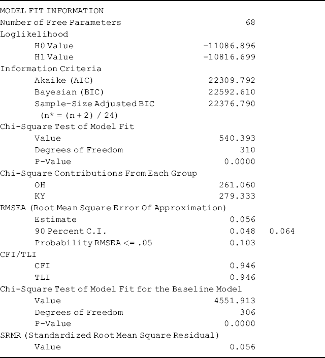
The strict measurement invariance model is to test invariance of all measurement parameters (i.e., factor loadings, item intercepts, and item variances) simultaneously. The current model needs to be compared with the configural model, in which no equality restrictions are imposed on any of those measurement parameters. The model difference between the two nested models is: χ² = (540.393 − 455.197) = 85.196 with df = (310 − 259) = 51, and P = 0.0019. Thus, we conclude that the hypothesis of the strict measurement invariance is rejected. We may also conduct another LR test by comparing the strict measurement invariance model with the strong measurement invariance model to examine how much change in the model statistic is attributed to equality restrictions on item variances. The corresponding χ² = (540.393 − 497.853) = 42.54 with df = (310 − 292) = 18, and P = 0.0009. This result indicates that item variances are noninvariant across groups.

Note that rejecting the hypothesis of strict measurement invariance does not mean the BSI-18 items are problematic, but only implies that the amount of variances of the observed item responses that are unexplained by their underlying factors are noninvariant across groups. What is important from the above invariance testing is that we have demonstrated metric and scalar invariance; thus we can proceed to test invariance of structural parameters, such as factor variance invariance, factor covariance invariance, and factor mean invariance.

Testing factor variance invariance: Factor variance invariance implies that the factors or latent constructs have the same distribution dispersions across groups. Assuming strong measurement invariance, we express the factor variance invariance model as:

(5.9)

(5.10)

where factor loadings () and item intercepts () are restricted to be invariant across groups. denotes that factor covariances (i.e., the off diagonals in ) are noninvariant across groups, while factor variances (i.e., the diagonals in ) are restricted to be invariant.

No equality restriction is imposed in the error variances () based on the findings in the strict measurement variance test. As in previous models, the model will be estimated based on analysis of MACS with factor means () being set to zero.

Mplus Program 5.8

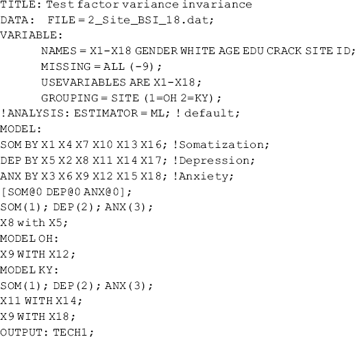
In Mplus Program 5.8, in addition to equality restrictions on factor loadings and item intercepts, the statements of SOM(1), DEP(2), and ANX(3) in both the overall MODEL command and the group specific MODEL KY command for Kentucky set the variances of factors SOM, DEP, and ANX invariant across groups. Selected model results are shown in Table 5.8.

Table 5.8 Selected Mplus output: testing factor variances invariance.

Regarding model comparison, a different reference model might be chosen depending upon the different perspectives of comparison. If we perceive factor variance invariance in addition to the strong measurement invariance (i.e., factor loading invariance and item intercept invariance), then the current model may be compared with the strong measurement invariance model, resulting in a LR = (502.245 − 497.853) = 4.392 with df = (295 − 292) = 3, P = 0.2221, and = (0.952 − 0.951) = 0.001. We may also use the configural model as the reference model for model comparisons because a model with multiple restrictions (invariant factor loadings, item intercepts, and factor variances across groups) should be compared with the corresponding model without such restrictions. The difference between the current model and the configural model is: = (502.245 − 455.197) = 47.048 with df = (295 − 259) = 36, which is not statistically significant (P = 0.1029). In addition, change in CFI between the two models is = (0.954 − 0.951) = 0.003, which is much smaller than the cut-off point of 0.01. We, therefore, conclude the factor variances are invariant across groups.

Given factor variance invariance, the group differences of the item variances are only attributed to the group difference of the random error variances. In other words, under the condition of factor variance invariance, the results of testing error variance invariance can be used to examine invariance of item reliabilities (Rock, Werts, and Flaugher, 1978; Cole and Maxwell, 1985; Vandenberg and Lance, 2000). In our example, we have tested that the factor variances are invariant, but the item variances are noninvariant, across groups. We, therefore, can conclude that the item reliabilities of SBI-18 are noninvariant when applied to rural drug using populations in Ohio and Kentucky.

Test factor covariance invariance: Assuming strong measurement invariance, we express factor covariance invariance model as:

(5.11)

(5.12)

where factor loadings () and item intercepts () are restricted to be invariant across groups; factor variances (i.e., the diagonals in ) are noninvariant across groups, while factor covariances (i.e., the off diagonals in ) are restricted to be invariant.

As in previous models, no equality restriction is imposed on the error variances () and factor means () are set to zero.

Mplus Program 5.9

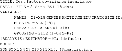
where the statements SOM with DEP(1), SOM with ANX(2), and DEP with ANX(3) in the overall MODEL command impose equality restrictions on the three factor covariances, respectively. Selected model results are shown in Table 5.9.

Table 5.9 Selected Mplus output: testing factor covariance invariance.

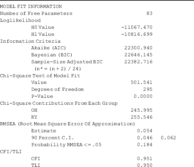
To compare the current model with the configural model, the LR = (501.541 − 455.197) = 46.344 with df = (295 − 259) = 36, which is not statistically significant (P = 0.1159); and change in CFI between the two models is = (0.954 − 0.951) = 0.003. We, therefore, conclude that the factor covariances of the SBI-18 are invariant between the Ohio and Kentucky rural drug using populations. In order words, the same relationships between the three constructs (i.e., depression, anxiety, and somatization) measured by the SBI-18 remain among the target populations in the two states.

Of course, factor variance and covariance invariance can be tested simultaneously. The LR test results are: = (505.414 − 455.197) = 50.217, df = (298 − 259) = 39, and P = 0.1076. We leave such a test for interested readers to practice.

Test factor mean invariance: The covariance structure and the mean structure for testing factor mean invariance can be described as:

(5.13)

(5.14)

where measurement parameters, such as factor loadings and item intercepts are set invariant across groups. Since the absolute values of the factor means cannot be estimated in multi-group CFA, group differences in factor means are modeled by treating one group as the reference group, against which factor means for the other groups are compared (Byrne, 2001, 2006; Bentler, 2005). In Equation (5.14) the factor mean vector () in fact represents the difference in factor means between the groups.

Mplus Program 5.10

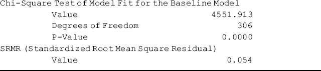
where factor loadings and item intercepts are set invariant across groups by default. The statement [SOM@0 DEP@0 ANX@0] is removed from the overall MODEL command to release the zero restrictions on factor means. By default, the first group (Ohio sample in this example) is treated as the reference group, for which all factor means are set to zero. The factor ‘means’ estimated for other groups (Kentucky sample in this example) are in fact differences in factor means between the groups and the reference group. The model results show specific statistical tests for differences in the factor means between groups.

Table 5.10 shows that factor means of SOM (−0.152, P = 0.013) and ANX (−0.207, P = 0.030) are significantly lower in Kentucky than in Ohio, while the factor mean of depression (DEP) is not significantly different between the two samples (−0.064, P = 0.489). In other words, somatization and depression scores among rural drug users measured by BSI-18 were significantly higher in Ohio than in Kentucky; however, the anxiety scores were not significantly different between the two states.

Table 5.10 Selected Mplus output: testing factor means invariance.

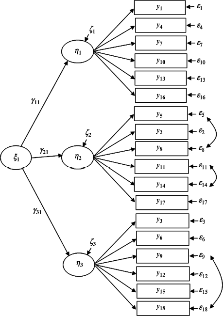
5.1.2 Multi-Group Second-Order CFA

In the previous sections our focus was on evaluation of measurement invariance in a first-order CFA model. Now we turn to evaluation of measurement invariance in a second-order CFA model using the same BSI-18 data. In our example model, the first-order factors (e.g., SOM, DEP, and ANX) are highly correlated with each other, and a general psychological distress – global severity index (GSI) can be theoretically hypothesized to account for the covariance among the first-order factors. In the following sections, second-order CFA models based on the three first-order factors are evaluated to account for a hierarchical factorial structure of the BSI-18. Figures 5.3 and 5.4 show the baseline second-order CFA models for Ohio and Kentucky, respectively, in which the observed indicator variables (i.e., the BSI-18 items) are denoted as y₁ − y₁₈, instead of x₁ − x₁₈. In a second-order CFA model, the first-order factors are indicators of the second-order factors, and thus the former are treated as endogenous latent variables (), and the latter are treated as exogenous latent variables (). Correspondingly, the indicators of the first-order factors are treated as endogenous indicators y₁ − y₁₈, and their error terms are denoted as , respectively, in Figures 5.3 and 5.4.

Figure 5.3 Second-order CFA model: Ohio.

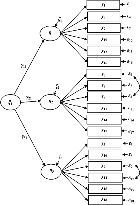
Figure 5.4 Second-order CFA model: Kentucky.

The principles of testing factorial invariance in a second-order CFA model remain the same as those in the first-order CFA model. We will start with testing second-order configural invariance of the BSI-18, and then test invariance of the second-order measurement parameters (e.g., the second-order factor loadings, intercepts of the first-order factors); and invariance of the second-order structural parameters (second-order factor variance, second-order factor mean).

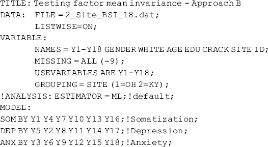
Second-order configural CFA model: As in testing factorial invariance in the first-order CFA, we first test the configural invariance of the second-order CFA. The first-order part of the model is set the same as the first-order configural CFA model in Section 5.1.1. In the second-order part of the model, the measurement parameters (e.g., second-order factor loadings, intercepts of the first-order factors, and residual variances of the first-order factors) and structural parameters (e.g., variance and mean of the second-order factor) are all treated as free parameters in the configural model. Covariances between the residual terms of the first-order factors are all set to zero because correlation between the first-order factors is supposed to be explained theoretically by the second-order factor on the one hand, and more importantly, for the purpose of model identification in our example model on the other hand. In a higher-order CFA model, both the lower-order and higher-order parts of the model must be identified. The first-order part of our model has three factors, each of which has six items, therefore, it is identified. The second-order part of the model is actually a single factor (i.e., GSI) CFA model with only three indicators (i.e., the first-order factors SOM, DEP, and ANX). From Chapter 2 we know that such a model is just-identified if no error covariance is specified.⁷ To make the second-order factorial structure of our model identifiable, the first-order factor residual covariances should all be set to zero. The following Mplus program implements the second-order configural CFA model.

Mplus Program 5.11

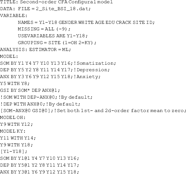
where the first-order factors (SOM, DEP, and ANX) are specified as indicators of the second-order factor GSI in both the Ohio and Kentucky samples. By respecifying the item intercepts and the first- and second-order factor loadings in group-specific MODEL KY command, it releases the default invariance restrictions on these parameters. Like the lower-order factors, the scale of the second-order factor GSI can be defined by either setting the variance of GSI to 1.0 or setting one of the factor loadings to 1.0. In Mplus Program 5.11, the factor loading of ANX is set to 1.0.⁸

In analysis of MACS, the total number of estimated intercepts (including intercepts of observed variables and intercepts of the first-order factors) and factor means must not be greater than the total number of observed variables (Bentler, 2005). As all the intercepts of the observed variables in this example are set free to estimate, all the intercepts of the first-order factors (SOM, DEP, and ANX), and the mean of the second-order factor (GSI) must be set to zero in order to avoid model un-identification. This is done by the statement [SOM-ANX@0 GSI@0] in the overall MODEL command. In addition, in the second-order part of the model, the residual covariances between the first-order factors must be set to 0 for the purpose of model identification, and this had to be done manually in early versions of Mplus. Very often researchers forgot to do so when testing a second-order CFA model with only three first-order factors, thus ending up with an error message in Mplus output such as the following:

Since Mplus version 6 the first-order factor residual covariances are set to 0 by default. This helps to avoid an often encountered programming problem among SEM beginners. The model results are shown in Table 5.11.

Table 5.11 Selected Mplus output: second-order configural CFA model.

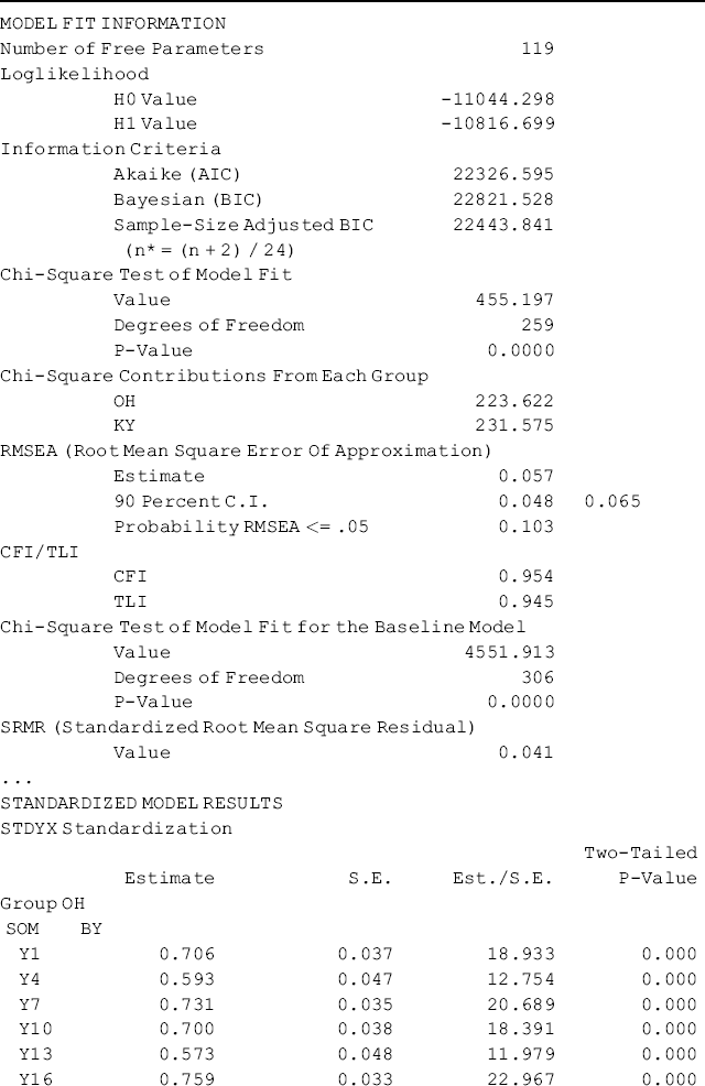
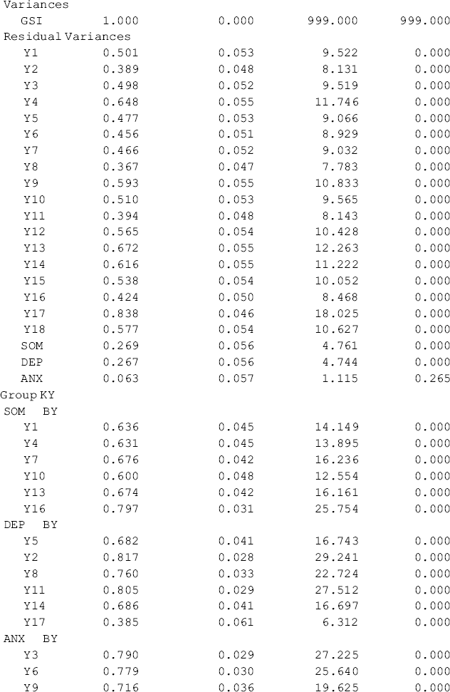
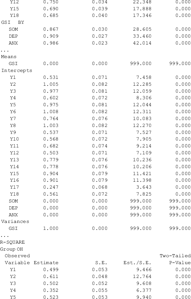
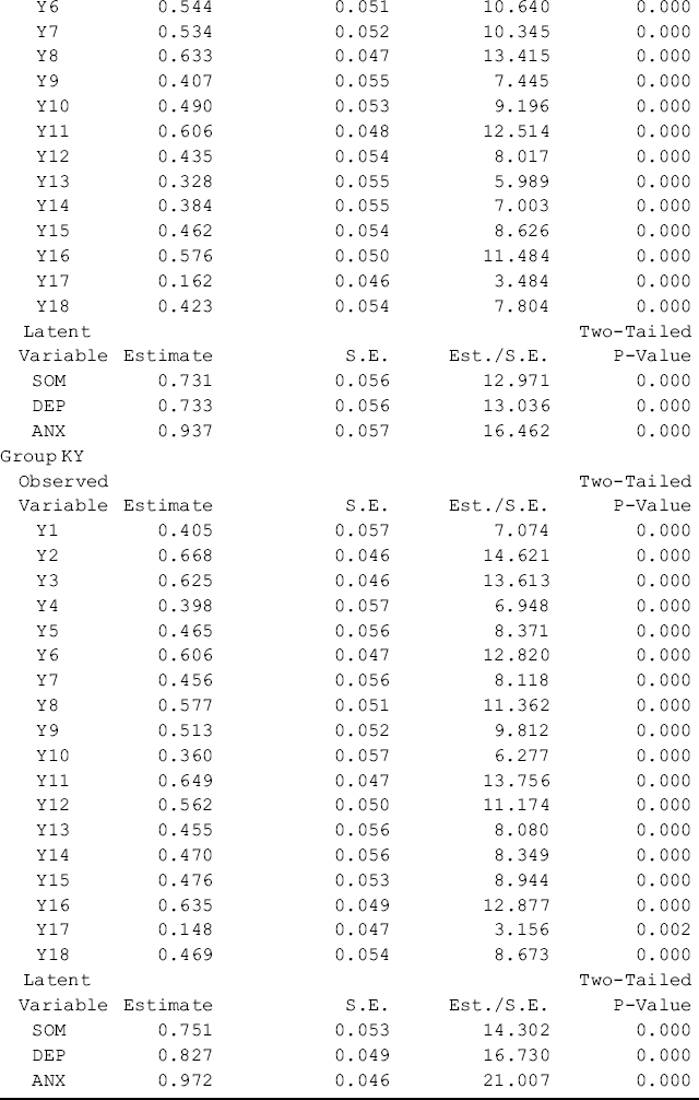
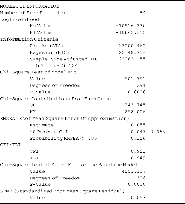
Table 5.11 shows that first- and second-order factor loadings, as well as intercepts of the observed variables/items are all estimated without across-group equality restrictions. The first-order factors are highly loaded on the second-order factor with factor loadings above 0.85. The portions of variation in the first-order factors explained by the second-order factor are high with R-Squared ranging from 0.731 to 0.937 for Ohio and from 0.751 to 0.972 for Kentucky, respectively. The second-order factor can be considered as a broader construct (GSI) of distress underlying the three first-order factors (SOM, DEP, and ANX) in both the Ohio and Kentucky samples. The model fits data very well: RMSEA = 0.057, 90% CI = (0.048, 0.065), close-fit test P = 0.103; CFI = 0.954, TLI = 0.945, and SRMR = 0.041.⁹

The results of the model provide the baseline values, to which the subsequently specified restricted models are compared.

Test invariance of second-order factor loadings: In addition to equality restrictions on the first-order factor loadings and item intercepts, we need to impose further equality restrictions on the second-order factor loadings, and then compare the model χ² statistics between the current model and the second-order configural CFA model.

Mplus Program 5.12

where the first-order measurement model is specified in the overall MODEL command, and not respecified in the group-specific MODEL commands, thus the first-order factor loadings and item intercepts are restricted equally across groups by default. However, no equality restrictions are imposed on second-order factor loadings by default in Mplus. To restrict them invariant across groups, we need to place the same symbol (e.g., a number or letter) in parentheses following each of the second-order factors in the overall MODEL command. Note that only one restriction is allowed on a line, otherwise Mplus will produce an error message. Selected model results are shown in Table 5.12.

Table 5.12 Selected Mplus output: testing invariance of second-order factor loadings.

Comparing the model results with those in Table 5.11, the model χ² change is: = (501.751 − 455.197) = 46.438 with df = (294 − 259) = 35, which is not statistically significant (P = 0.0935). Change in CFI, = (0.954 − 0.951) = 0.003 is much smaller than 0.01. Thus, we conclude that the second-order factor loadings of our model are invariant across groups. Next, we proceed to test factor mean differences across groups.

Test invariance of factor means: In a second-order CFA model, testing factor mean differences involves testing invariance of the first-order factor intercepts and invariance of the second-order factor means. The mean structure of the second-order CFA model can be expressed as:

(5.15)

(5.16)

(5.17)

thus

(5.18)

where represents the vector of intercepts of the observed indicator variables, is the first-order factor loading matrix, is the matrix of second-order factor loadings, is the vector of the first-order factor intercepts (or means of the first-order factors, corresponding to zero value of the second-order factor mean), represents the vector of the second-order factor means, is the vector of measurement errors in the observed indicator variables, and is the vector of residuals of regressing first-order factors on the second-order factors. Equations (5.15) and (5.16) represent the first- and second-order factorial structures in the second-order CFA model. Substituting Equation (5.16) into Equation (5.15), we have Equation (5.17). Equation (5.18) is the mean structure of the model in which the means () of the observed variables are expressed in terms of observed variable intercepts (), the first-order factor intercepts (), and the second-order factor means ().

In a second-order CFA model the mean structure part of the model is generally not identified because the number of intercepts and means to estimate is more than the number of observed indicator variables. As such, parameter restrictions are needed to address the identification problems. Three different parameter restriction approaches (Approaches A, B, and C) are usually proposed for such a purpose (Byrne, 2006): (A) setting equality restriction on across groups, fixing and to zero in one group, and imposing further restrictions on or in other groups (Lubke, Dolan, and Kelderman, 2001); (B) fixing intercepts of some observed variables at some known values; and (C) fixing to zero in all groups.

Application of Approach A: For a two-group second-order CFA model, the mean structures defined by Approach A can be described as:

(5.19)

(5.20)

where the two equations are for Groups 1 and 2, respectively, in which the item intercepts (), the first-order factor loadings (), and the second-order factor loadings () are all set to be equal across groups; all first-order factor intercepts () and second-order factor means () are set to zero in Group 1, thus Equation (5.19) becomes . In our example, there are 2 × 18 = 36 observed variable means available for mean structure analysis, in which the parameters to estimate are: 18 item intercepts in Groups 1 and 2, three first-order factor intercepts in Group 2, and one second-order factor mean in Group 2. Thus the total number (36) of observed variable means is greater than the total number (18 + 3 + 1 = 22) of free parameters. However, this does not necessarily mean that the mean structure part of the model is identified because Equation (5.20) has an identification problem at the factor level. In this example, there are three first-order factors; i.e., there are only three pieces of mean structure information, but four parameters (i.e., three first-order intercepts and one second-order factor mean) to estimate in the second-order part of the model. In order to make it identifiable, at least one more restriction on or is needed. In this example we set the second-order factor mean () to zero in Group 2.

Mplus Program 5.13

where the intercepts of the observed indicator variables, the first-order factor loadings, and the second-order factor loadings are set equal across groups. The statement [SOM-ANX@0 GSI@0] in the overall MODEL command of Mplus Program 5.12 is replaced with statement [GSI@0] in Mplus Program 5.13. That is, the intercepts of the first-order factors are set to zero in the reference group (i.e., Group 1 or the Ohio sample in this example), but free to estimate in the second group (i.e., Group 2 or the Kentucky sample in this example), while the second-order factor means are set to zero in both groups. The model here is to assess invariance of the first-order factor intercepts (or differences in the means of the first-order factors, corresponding to the zero value of the second-order factor mean) between groups. The estimated intercepts/means of the first-order factors in the second group are in fact the differences in the intercepts/means between Groups 1 and 2.

Alternatively, we may free the second-order factor mean in Group 2 but impose equality restriction on any two first-order factor intercepts in Group 2. For example, replacing the statement [GSI@0] with [DEP ANX](E)¹⁰ in the group-specific MODEL KY command would make the model identifiable; however, we may not do so unless it is interpretable by forcing the intercepts of the first-order factors DEP and ANX to be equal in Group 2. For the current example, we set the mean of the second-order factor to zero and let the first-order factor intercept free because our focus here is to test invariance of the first-order factor intercepts.

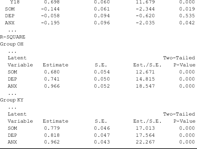
As Group 1 (Ohio) was treated as the reference group against which Group 2 (Kentucky) is compared, the estimates of the first-order factor intercepts for Ohio are all zeros, and the estimated first-order factor intercepts for Kentucky (i.e., −0.144, P = 0.019; −0.058, P = 0.535; and −0.195, P = 0.042, respectively) are in fact the group differences in the first-order factor intercepts (or the means of the first-order factors, corresponding to the zero value of the second-order factor) (see the intercept estimates in the Group KY section of Table 5.13). Consistent with the findings in the multi-group first-order CFA model (Table 5.10), the levels of somatization and anxiety among rural drug users in Kentucky were significantly lower than those in Ohio, but there was no significant difference in regard to depression level between the two populations, given the same level of second-order factor mean (i.e., the GSI).

Table 5.13 Selected Mplus output: testing invariance of factor means: Approach A.

Application of Approach B: The mean structure defined in Approach B can be described as:

(5.21)

(5.22)

where the first-order factor loadings (), second-order factor loadings (), and the first-order factor intercepts () are also set invariant across groups. Since three first-order factor intercepts are treated as free parameters in Equation (5.21), three item intercepts need to be fixed to make the equation at least just identified. The item intercept vector represents that some of the item intercepts are fixed to known values (e.g., estimated from previous model). This approach allows testing of invariance of the second-order factor means across groups. The corresponding Mplus program follows.

Mplus Program 5.14

where the intercepts of the last item in each of the three first-order factors (SOM, DEP, and ANX) in each group are set to known values ( = 1.597, = 0.261, and = 0.748) that are estimated from Mplus Program 5.12. The statement [SOM](S), [DEP](D), and [ANX](A) specified in the group specific MODEL OH command and the group-specific MODEL KY command impose equality restrictions on the first-order factor intercepts across groups.

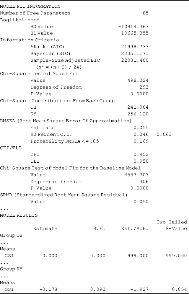
The model results show that the estimated mean of the second-order factor GSI for Kentucky = −0.178 (P = 0.054), which is in fact the estimated difference in mean of the second-order factor GSI between the two populations. In other words, the score of the GSI among rural drug users in Kentucky was 0.178 points lower on average than that in Ohio. However, the difference is only marginally significant (P = 0.054; Table 5.14).

Table 5.14 Selected Mplus output: testing invariance of factor means: Approach B.

Application of Approach C: In this approach, the first-order factor intercepts are all fixed to zero in both groups (i.e., = 0 and = 0), and the second-order factor mean () is set to zero in Group 1. The mean structure is described as:

(5.23)

(5.24)

where equality restrictions are imposed on the first-order factor loadings and item intercepts, and the first-order factor means are set to zero across groups. Parameter , the difference in mean of the second-order factor between groups, will be estimated.

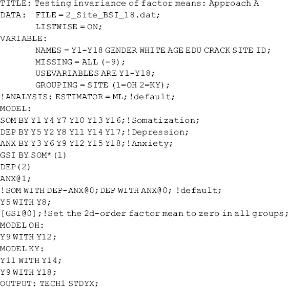
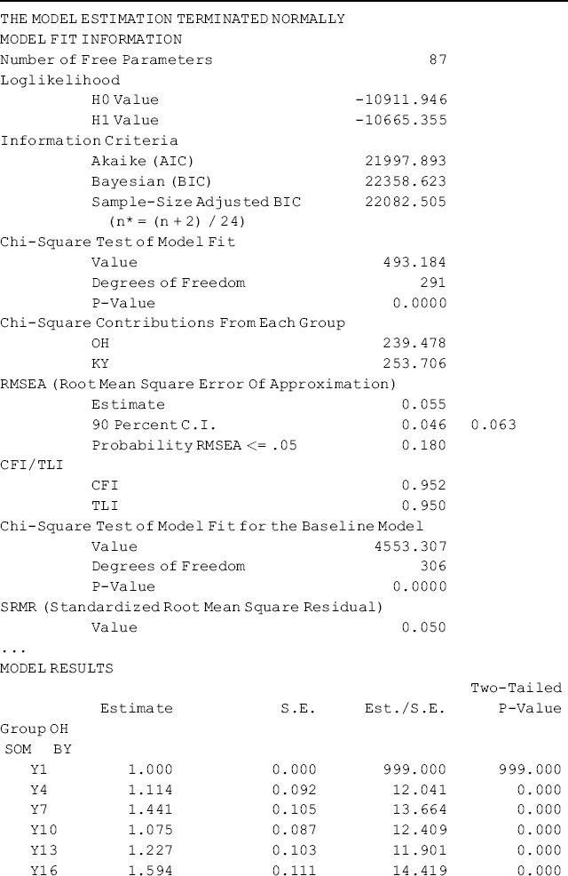
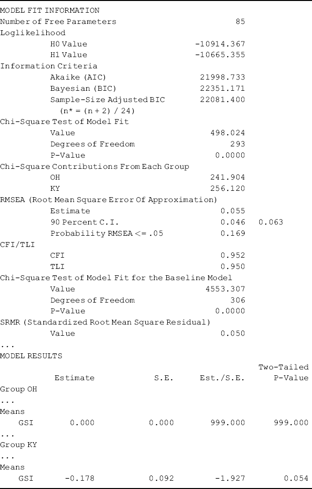
Mplus Program 5.15

where the statement [SOM-ANX@0] in the overall MODEL command sets the first-order factor intercepts to zero (i.e., = 0 and = 0) in all groups; the second-order factor mean for Group 1 () is set to zero by default. Approach C will produce an identical estimate of to that produced by Approach B (Byrne, 2006).

As expected, the difference in the second-order factor mean ( = −0.178, P = 0.054) estimated from Approach C (Table 5.15) is identical to that estimated from Approach B.

Table 5.15 Selected Mplus output: testing invariance of factor means: Approach C.

In this section we have discussed and demonstrated three different parameter restriction approaches (Approaches A, B, and C) to address the identification problems in testing factor mean differences in multi-group second-order CFA models. Approach A is suitable for testing invariance of first-order factor intercepts/means across groups, and both Approaches B and C are suitable for testing invariance of second-order factor means.