7.2 Satorra and Saris's Method for Sample Size Estimation
Satorra and Saris (1985) proposed an approach to estimate statistical power for SEM models. The idea behind the method is when a model is misspecified (but not severely so) the model fit test statistic does not follow a central χ2 distribution, but a noncentral χ2 distribution. The model χ2 statistic of the misspecified model can be considered as an approximation of the noncentrality parameter (![]() ) of the noncentral χ2 distribution (note, the
) of the noncentral χ2 distribution (note, the ![]() here is not the
here is not the ![]() that denotes factor loadings in our CFA models). Once the
that denotes factor loadings in our CFA models). Once the ![]() parameter has been estimated, statistical power can be obtained either from a table for noncentral χ2 distribution for specific degrees of freedom and
parameter has been estimated, statistical power can be obtained either from a table for noncentral χ2 distribution for specific degrees of freedom and ![]() level (Saris and Stonkhorst, 1984) or calculated using statistical packages, such as SAS or SPSS (Brown, 2006; http://www.statmodel.com/power.shtml).
level (Saris and Stonkhorst, 1984) or calculated using statistical packages, such as SAS or SPSS (Brown, 2006; http://www.statmodel.com/power.shtml).
Several steps are followed in application of Satorra and Saris's method to estimate statistical power and thus sample size (Brown, 2006):
In the following we will demonstrate how to use Mplus to implement Satorra and Saris's method to estimate sample size for assessing factor covariance in a CFA model and the rate of outcome change over time in a LGM.
7.2.1 Application of Satorra and Saris's Method to CFA model
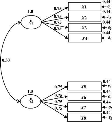
The hypothesized CFA model shown in Figure 7.1 involves two factors, ![]() and
and ![]() ; each has four indicators (x1–x4 for
; each has four indicators (x1–x4 for ![]() and x5−x8 for
and x5−x8 for ![]() ). All the indicators are assumed to have a mean of zero and a variance of 1.00. All factor loadings are specified as 0.75, indicating an item reliability of 0.56. For the purpose of defining factor scale, factor variances are specified as 1.0. As such, all error variances would be 1.00 − 0.56 = 0.44. The covariance between the two factors is hypothesized to be 0.30. All the parameter values specified in implementation of Satorra and Saris's method are hypothesized population parameter values based on the best theoretical guess or empirical findings. In our example, the parameter values are simply for the purpose of model demonstration.
). All the indicators are assumed to have a mean of zero and a variance of 1.00. All factor loadings are specified as 0.75, indicating an item reliability of 0.56. For the purpose of defining factor scale, factor variances are specified as 1.0. As such, all error variances would be 1.00 − 0.56 = 0.44. The covariance between the two factors is hypothesized to be 0.30. All the parameter values specified in implementation of Satorra and Saris's method are hypothesized population parameter values based on the best theoretical guess or empirical findings. In our example, the parameter values are simply for the purpose of model demonstration.
Figure 7.1 Hypothesized CFA for estimating statistical power and sample size.
The following Mplus program is for Step 1 of implementing Satorra and Saris's method for the CFA model.
Mplus Program 7.1
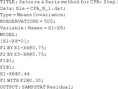
where the MEANS COVARIANCE option is specified in the TYPE statement of the DATA command to define data input type (MACS). A relatively large sample size N = 500 is specified in the NOBSERVATIONS statement of the DATA command. The data (data file CFA_N_1.dat) used for the modeling are in matrix format containing only null data that look like the following:
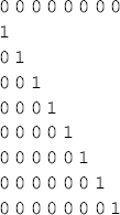
where the mean vector has all 0 cells, all variances are set to 1.0, and all covariances are set to 0. From Chapter 1 we know that the purpose of model fit in SEM is to find a set of model parameters to generate the model implied variance/covariance matrix ![]() , which is the estimated population covariance matrix; and minimize the discrepancy between the observed variance/covariance matrix S and the model implied variance/covariance matrix
, which is the estimated population covariance matrix; and minimize the discrepancy between the observed variance/covariance matrix S and the model implied variance/covariance matrix ![]() . Here we are using an inverse process; that is, the population mean vector and variance/covariance matrix are generated to correspond to the given parameterization of the model (i.e., each parameter in the model is fixed to its population value).
. Here we are using an inverse process; that is, the population mean vector and variance/covariance matrix are generated to correspond to the given parameterization of the model (i.e., each parameter in the model is fixed to its population value).
The RESIDUAL option specified in the OUTPUT command in Mplus Program 7.1 allows the production of the population mean vector and variance/covariance matrix that correspond to the population parameters specified in the program.
Table 7.1 shows that the model fits data poorly, which is not unexpected. The purpose of Mplus Program 7.1 is to generate the population mean vector and covariance matrix for later use, instead of fitting the model to the arbitrary null data. The population mean vector and variance/covariance matrix printed in Mplus output (Table 7.1) look like the following:
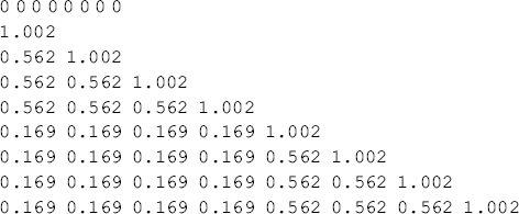
Table 7.1 Selected Mplus output: Satorra and Saris's method Step 1.
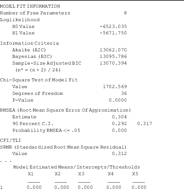
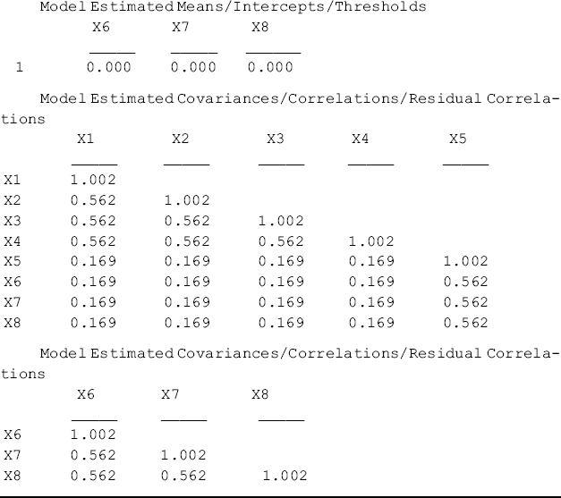
This MACS is saved in data file CFA_N_2.dat 2 and will be used for the next modeling. Using the generated population mean vector and variance/covariance matrix as data input, Step 2 of Satorra and Saris's method estimates the model parameters and checks whether the estimated parameters match those specified in Step 1. The corresponding Mplus program follows:
Mplus Program 7.2
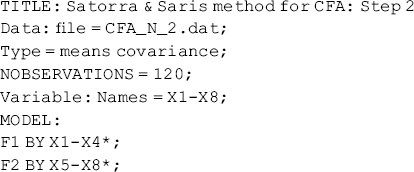

where model parameters are set free to estimate and a moderate sample size (N = 120) is specified. The estimated model parameters are shown in Table 7.2.
Table 7.2 Selected Mplus output: Satorra and Saris's method Step 2.
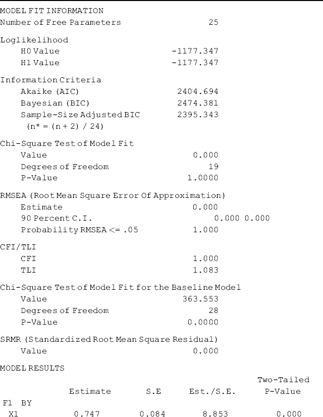
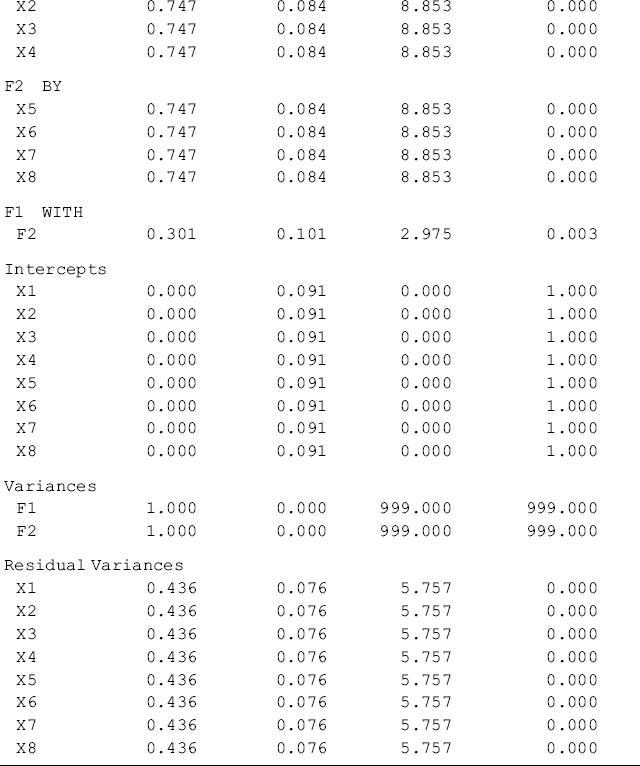
Table 7.2 shows that the model fits data perfectly. This is because the ‘population’ MACS, instead of a sample MACS, is used as data input for modeling. From Table 7.2 we can see that the parameter estimates are almost identical to the population parameter values specified in Step 1 in Mplus Program 7.1. This indicates that the parameter estimates with the theoretical expectations match very well. As such, we can go ahead to implement Step 3 of Satorra and Saris's method in the following Mplus program, which models a misspecified model.
Mplus Program 7.3
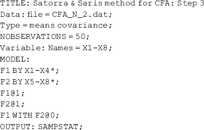
where the generated population mean vector and covariance matrix (data file CFA_N_2.dat) is used as data input. The statement NOBSERVATIONS = 50 in the DATA command sets sample size to N = 50. Since our interest is to test the significance of the factor covariance (i.e., ![]() ), this covariance parameter is misspecified to 0 on purpose, using the statement F1 with F2@0 in the MODEL command. The model χ2 statistic estimated from this misspecified model is
), this covariance parameter is misspecified to 0 on purpose, using the statement F1 with F2@0 in the MODEL command. The model χ2 statistic estimated from this misspecified model is ![]() = 3.267, which can be treated as an approximate noncentrality parameter
= 3.267, which can be treated as an approximate noncentrality parameter ![]() . In a table for noncentral
. In a table for noncentral ![]() distribution, we can find the corresponding statistical power is about 0.44. The power can also be readily calculated using the statistical package SAS as shown in the following. Clearly, N = 50 is not large enough to reject the false hypothesis
distribution, we can find the corresponding statistical power is about 0.44. The power can also be readily calculated using the statistical package SAS as shown in the following. Clearly, N = 50 is not large enough to reject the false hypothesis ![]() = 0 and detect the factor covariance
= 0 and detect the factor covariance ![]() = 0.30. Then we have to run Mplus Program 7.3 repeatedly with sample size varying from N = 50 to N = 150.3 The estimated noncentrality parameter values are then used to compute the values of statistical power corresponding to different sample sizes in the following SAS program.
= 0.30. Then we have to run Mplus Program 7.3 repeatedly with sample size varying from N = 50 to N = 150.3 The estimated noncentrality parameter values are then used to compute the values of statistical power corresponding to different sample sizes in the following SAS program.
SAS Program 7.1
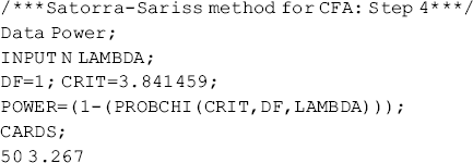
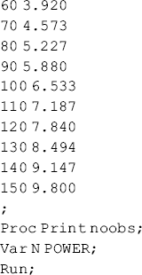
where variable LAMBDA represents the approximate values of the noncentrality parameters ![]() estimated from the misspecified model with different sample sizes. CRIT = 3.841 is the
estimated from the misspecified model with different sample sizes. CRIT = 3.841 is the ![]() statistic value for df = 1 at level of
statistic value for df = 1 at level of ![]() = 0.05.
= 0.05.
The estimated values of the statistical power corresponding to different sample sizes are shown in Table 7.3. A sample with N = 120 or larger would have a power of 0.80 or larger to detect the hypothesized factor covariance ![]() = 0.30 in the hypothesized two-factor CFA model.
= 0.30 in the hypothesized two-factor CFA model.
Table 7.3 Estimated statistical power by sample size using Satorra and Saris's method for testing factor covariance in a CFA model.
| Sample size (N) | Power |
| 50 | 0.44 |
| 60 | 0.51 |
| 70 | 0.57 |
| 80 | 0.62 |
| 90 | 0.67 |
| 100 | 0.72 |
| 110 | 0.76 |
| 120 | 0.80 |
| 130 | 0.83 |
| 140 | 0.86 |
| 150 | 0.88 |
7.2.2 Application of Satorra and Saris's Method to a LGM
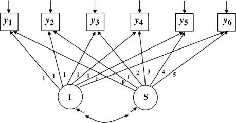
In this section the same process implemented in Section 7.2.1 is used to demonstrate application of Satorra and Saris's method to an unconditional linear LGM with six repeated outcome measures (y1 − y6) (Figure 7.2). First, the following null
MACS data set is saved in data file LGM_N_1.dat and used as data input in Mplus Program 7.4 to generate the population MACS:
Figure 7.2 Hypothesized unconditional LGM for estimating statistical power and sample size.

Mplus Program 7.4

In Mplus Program 7.4 the population mean value of the baseline outcome measure is assumed to be 0.2 with a variance of 0.3 (i.e., the latent intercept growth factor ‘I’ has a mean of 0.2 and a variance of 0.3). Assuming a linear growth trajectory, the time scores are set to 0, 1, 2, 3, 4, and 5, respectively, for the six time points. The rate of outcome change is assumed as 0.1 with a variance of 0.1 (i.e., the latent slope growth factor ‘S’ has a mean of 0.1 and a variance of 0.1). The two latent growth factors (‘I’ and ‘S’) are associated with each other, assuming a covariance of 0.1. The residual variances are assumed to be 0.5 for all the observed outcome measures (y1–y6). Again, the RESIDUAL option is specified in the OUTPUT command to generate the population MACS that looks like the following:
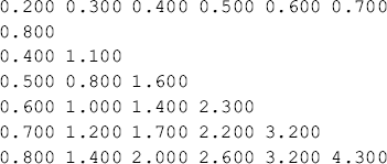
This generated population MACS is saved in data file LGM_N_2.dat and used as data input in the following Mplus program, in which the same model is implemented to check whether the parameter estimates match the population values of the parameters specified in Mplus Program 7.4.
Mplus Program 7.5
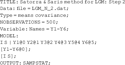
The model output (not reported here) of Mplus Program 7.5 shows that the model estimated parameter estimates match their hypothesized population values very well. So, the next step is to run the misspecified model to estimate the noncentrality parameter ![]() . Since our interest here is to estimate an adequate sample size that ensures a large enough statistical power to detect a significant outcome change, indicated by the slope growth factor S, we set S = 0 as the null hypothesis of no significant outcome change in the misspecified model. The purpose is to determine a sample size that allows us to reject this null hypothesis with a power of at least 0.80. In the following Mplus program, we estimate the noncentrality parameter staring with N = 50.
. Since our interest here is to estimate an adequate sample size that ensures a large enough statistical power to detect a significant outcome change, indicated by the slope growth factor S, we set S = 0 as the null hypothesis of no significant outcome change in the misspecified model. The purpose is to determine a sample size that allows us to reject this null hypothesis with a power of at least 0.80. In the following Mplus program, we estimate the noncentrality parameter staring with N = 50.
Mplus Program 7.6
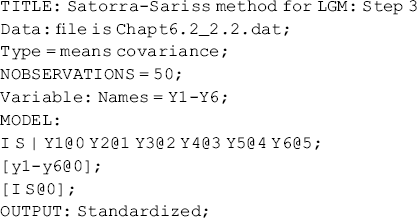
where statement [I S@0] in the MODEL command misspecifies the mean of the latent slope growth factor by setting S to 0. The estimated model ![]() statistic is the estimated noncentrality parameter
statistic is the estimated noncentrality parameter ![]() = 3.819. The same program is run multiple times with different sample size ranging from N = 50 to N = 150. The
= 3.819. The same program is run multiple times with different sample size ranging from N = 50 to N = 150. The ![]() parameter estimates are then input in SAS Program 7.2 to calculate the corresponding values of statistical power. Table 7.4 shows that a sample size of N = 110 is needed in order to have a power of greater than 0.80 to detect a rate of outcome change of 0.10 in the designed LGM.
parameter estimates are then input in SAS Program 7.2 to calculate the corresponding values of statistical power. Table 7.4 shows that a sample size of N = 110 is needed in order to have a power of greater than 0.80 to detect a rate of outcome change of 0.10 in the designed LGM.
Table 7.4 Estimated statistical power by sample size using Satorra and Saris's method for testing rate of outcome change in a LGM.
| Sample size (N) | Power |
| 50 | 0.50 |
| 60 | 0.57 |
| 70 | 0.64 |
| 80 | 0.69 |
| 90 | 0.74 |
| 100 | 0.79 |
| 110 | 0.82 |
| 120 | 0.85 |
| 130 | 0.88 |
| 140 | 0.90 |
| 150 | 0.92 |
SAS Program 7.2


The same process demonstrated above can be applied to other SEM models. The key limitation of Satorra and Saris's method is that it must specify both null and alternative models that are nested, and can only test the null hypothesis in regard to the restricted parameter(s). An increasingly applied approach for power analysis and sample size estimate for SEM is Monte Carlo simulation that can provide statistical power estimates, as well as precision information, for all free parameters involved in a model given a sample size. In the next section we will discuss and demonstrate Monte Carlo simulation for the same CFA model and LGM demonstrated in this section and will compare the results of the Monte Carlo simulation with those of Satorra and Saris's method. In addition, a covariate (e.g., intervention) and missing values caused by different attrition rates in longitudinal data will be considered in the LGM.
