5.2 Proofs for Section 4.4 “The Bifrequency Cross-Periodogram”

In this section, proofs of lemmas and theorems presented in Section 4.4 on bias and covariance of the bifrequency cross-periodogram are reported.

The following Lemma 5.2.1 allows, in the proofs of the subsequent lemmas and theorems, the free interchange of the order of limit and sum operations.

Lemma 5.2.1 (Napolitano 2003, Lemma A.1).

a. Under Assumption 4.4.3a (series regularity), the function series is uniformly convergent. Moreover, for any function sequence of uniformly bounded functions the function series is uniformly convergent.

b. Under Assumption 4.4.3b (series regularity), the function series

is uniformly convergent. Moreover, for any function sequence of uniformly bounded functions, the function series

is uniformly convergent.

Proof: The uniform convergence of the function series is an immediate consequence of (4.97) and the Weierstrass criterium (Smirnov 1964). Moreover, since the functions are uniformly bounded, accounting for (4.97), it results in and hence, for the Weierstrass criterium the function series turns out to be uniformly convergent. Part b) of the Lemma can be proved analogously.

5.2.1 Proof of Lemma 4.4.6 Expected Value of the Bifrequency Cross-Periodogram

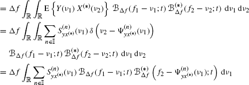
By substituting into (4.93) the STFTs and expressed according to (4.94b), and taking the expected value, one has

(5.6)

where, in the third equality, (4.95) with z₁ = y and z₂ = x^(*) is used.

In the derivation of (5.6), the order of integral and expectation operators can be interchanged due to the Fubini and Tonelli theorem (Champeney 1990, Chapter 3). In fact, defined

(5.7)

and accounting for Assumptions 4.4.3a and 4.4.5, for the integrand function in the right-hand side of (5.6) we have

(5.8)

The interchange of sum and integral operations to obtain (4.106) from (5.6) is justified even if the set is not finite by using the dominated convergence theorem (Champeney 1990, Chapter 4). Specifically, by denoting with an increasing sequence of finite subsets of , i.e., such that for h < k and , we have

(5.9)

In fact, it results that

(5.10)

with the right-hand side bounded by the right-hand side of (5.8). That is, the integrand function in the second term of equality (5.9) is bounded by a summable function of ν₁ not depending on k.

5.2.2 Proof of Lemma 4.4.7 Covariance of the Bifrequency Cross-Periodogram

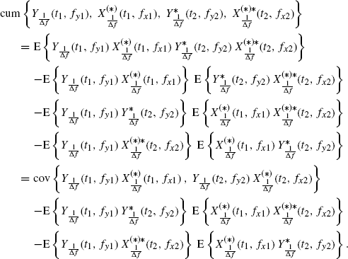
For zero mean stochastic processes x(t) and y(t), also the STFTs and are zero mean. By specializing to N = 4 and zero-mean processes the expression of Nth-order cumulant in terms of Nth-and lower-order moments (4.39), the result is that

(5.11)

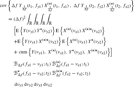
Thus, accounting for the STFT expression (4.94b), from (5.11) it follows that

(5.12)

Finally, by substituting (4.95) and (4.96) into (5.12), and using the sampling property of the Dirac delta, (4.108) follows.

The interchange of expectation, sum, and integral operations can be justified as in the proof of Lemma 4.4.6.

Lemma 5.2.2 (Napolitano 2003, Lemma A.2). Let Ψ⁽ⁿ⁾(f₁) be a function satisfying Assumption 4.4.4 (support-curve regularity (I)). For any function V(ν) continuous a.e. and infinitesimal at ±∞, one has

(5.13)

for any λ₁ such that is a continuity point of V.

Proof. If f₂ ≠ Ψ⁽ⁿ⁾(f₁), then f₂ ≠ Ψ⁽ⁿ⁾(f₁) definitively in a neighborhood of f₁ since Ψ⁽ⁿ⁾ is derivable and, hence, continuous. Thus, one has

(5.14)

from which it follows that

(5.15)

since V(ν) is continuous a.e. and infinitesimal at ±∞. Furthermore, if f₂ = Ψ⁽ⁿ⁾(f₁) then, from the assumption of derivability of Ψ⁽ⁿ⁾(f₁), one has

(5.16)

Thus, (5.13) follows from the a.e. continuity of V.

Lemma 5.2.3 (Napolitano 2003, Lemma A.3). Let and be second-order harmonizable jointly SC stochastic processes with bifrequency cross-spectrum (4.15), and define the function

(5.17)

Under Assumptions 4.4.3a (series regularity), 4.4.4 (support-curve regularity (I)), and 4.4.5 (data-tapering window regularity), one obtains

(5.18)

with E⁽ⁿ⁾(f₁) defined in (4.113).

Proof. By making into (5.17) the variable change λ₁ = (f₁ − ν₁)/Δf and accounting for (4.103) and (4.107) one has

(5.19)

Denoted by G_Δf(λ₁) the integrand function in (5.19) and accounting for (4.97) and Assumption 4.4.5, the result is that

(5.20)

with the right-hand side independent of Δf. Thus, the dominated convergence theorem (Champeney 1990) can be applied:

(5.21)

where, in obtaining (5.21), the limit (as Δf → 0) and the sum (over n) operations can be interchanged since W_B is bounded (Assumption 4.4.5) and hence, by Lemma 5.2.1a, the integrand function series in (5.19) is uniformly convergent. Moreover, the sum and the integral operations can be interchanged due to the same arguments used in the proof of Lemma 4.4.6. Furthermore, since and is regular at ±∞, then is infinitesimal at ±∞. Thus, by substituting (5.13) (Lemma 5.2.2) with V = W_B into (5.21) for all except, possibly, the λ₁s belonging to a set with zero Lebesgue maesure, (5.18) immediately follows.

Observe that, strictly speaking, to prove Lemmas 4.4.6, 5.2.1, and 5.2.3, Assumptions 4.4.3a and 4.4.4 need to hold only for z₁ = y and z₂ = x^(*).

5.2.3 Proof of Theorem 4.4.8 Asymptotic Expected Value of the Bifrequency Cross-Periodogram

It immediately follows from Lemma 5.2.3 for t₁ = t₂ = t.

5.2.4 Proof of Theorem 4.4.9 Asymptotic Covariance of the Bifrequency Cross-Periodogram

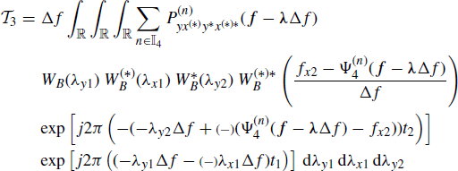
The asymptotic covariance expression (4.115) is obtained from (4.108) as Δf → 0. In fact, the convergence, as Δf → 0, of the terms and (see (4.109) and (4.110)) to and (see (4.116) and (4.117)), respectively, can be easily proved by using Lemma 5.2.3. Moreover, the term (see (4.111)) approaches zero as Δf → 0. In fact, by making into (4.111) the variable changes λ_y1 = (f_y1 − ν_y1)/Δf, λ_x1 = (f_x1 − ν_x1)/Δf, λ_y2 = (f_y2 − ν_y2)/Δf and accounting for (4.103) and (4.107), one has

(5.22)

where f − λΔf [f_y1 − λ_y1Δf, f_x1 − λ_x1Δf, f_y2 − λ_y2Δf].

Denoted by H_Δf(λ_y1, λ_x1, λ_y2) the integrand function in (5.22) and accounting for (4.98) and Assumption 4.4.5 the result is that

(5.23)

with the right-hand side independent of Δf. Thus,

(5.24)