Chapter 4 Linear Induction Motors: Circuit Theories, Transients, and Control

Search in book...
Toggle Font Controls
Create new playlist

Name your new playlist

Playlist description (optional)
Sign In

Email address

Password

Forgot Password?

or

Continue with Facebook

Continue with Google
Sign Up

Full Name

Email address

Confirm Email Address

Password

or

Continue with Facebook

Continue with Google

Circuit Theories, Transients, and Control

4.1 Low-Speed/High-Speed Divide

Field theories presented in Chapter 3 proved static and dynamic end effects as the main differences between rotary and linear induction motors.

Other specific phenomena related to the conductive sheet (alone or one placed on solid iron) such as edge effects, besides skin effect, airgap fringing, and primary slot opening influence on performance, have been reduced to equivalent correction coefficients on airgap (g_e) and on secondary sheet electrical conductivity σ_e.

The dynamic end effect divides the LIMs into high-speed (when this effect counts) and low-speed LIMs when the dynamic end effect is negligible. It is not so easy to hammer out a border between the two cases, but a first approximation would be to consider a LIM as of low speed if the exit end wave penetration depth along motion direction 1/γ₂_r (3.61–3.62) is less than 10% of primary length (2 · p · τ):

1 γ 2 r < 2 \cdot p \cdot τ 10 (4.1)

$\frac{1}{γ_{2 r}} < \frac{2 \cdot p \cdot τ}{10} (4.1)$

As γ₂_r depends on the equivalent goodness factor G_e, slip S, and pole pitch τ [1],

γ 2 r = a 1 2 (1 - 1 + b 1 2 - - - - - - \sqrt) (4.2)

$γ_{2 r} = \frac{a_{1}}{2} (1 - \sqrt{\frac{1 + b_{1}}{2}}) (4.2)$

a 1 = π τ \cdot G e \cdot (1 - S); b 1 = 1 + 16 G 2 e \cdot ( 1 - S ) 4 - - - - - - - - - - - - - - \sqrt (4.3)

$a_{1} = \frac{π}{τ} \cdot G_{e} \cdot (1 - S); b_{1} = \sqrt{1 + \frac{16}{G_{e}^{2} \cdot {(1 - S)}^{4}}} (4.3)$

Condition (4.1) becomes

p \cdot π \cdot G e \cdot (1 - S) \cdot (1 - 1 + b 1 2 - - - - - - \sqrt) > 10 (4.4)

$p \cdot π \cdot G_{e} \cdot (1 - S) \cdot (1 - \sqrt{\frac{1 + b_{1}}{2}}) > 10 (4.4)$

As this condition depends only on equivalent goodness factor G_e, slip S, and number of poles 2p, it may be simply represented on a fairly general graph (Figure 4.1).

The intersection of continuous and interrupted lines in Figure 4.1 for a given slip S suggests compliance with condition (4.1).

For example, at S = 0.1, for 2p = 4, 6, 8, there is no low-speed solution but for 2p = 10 there is one with large G_e (and good performance): G_e = 21.

Also for 2p = 12, S = 0.05, there is a solution at G_e = 25; for S = 0.1 and for 2p = 12, a larger G_e is allowed (G_e = 35!). Values of G_e larger than 25 correspond in general to well-designed highspeed LIMs (100–110 m/s): the optimum goodness factor G_e for 2p = 12 is G_e₀ = 27 in Figure 3.26.

Images

FIGURE 4.1 Exit end effect wave (interrupted lines) penetration depth per pole pitch versus G_e for given p and S (slip). (After Boldea, I. and Nasar, S.A., Linear Motion Electromagnetic Devices, Taylor & Francis, New York, 2001.)

Therefore, the optimal goodness factor is rather close to the condition that the penetration depth of exit end effect wave equals only 10% of primary length; this means that, grossly, the end effect influence on thrust reduction at rated slip is less than 10%.

Now we may proceed to the investigation of circuit models, transients, and control of low-speed LIMs as they resemble rotary IMs, though dedicated circuit parameter expressions for flat (and tubular) LIMs with Al-on-iron and for ladder secondary have to be derived.

4.2 Lim Circuit Models without Dynamic end Effect

There are a few basic topologies for low-speed LIMs:

Flat DLIMs with Al sheet secondary
Flat SLIMs with Al-on-iron secondary
Flat SLIMs with ladder secondary
Tubular SLIMs with cage secondary

We will derive the equivalent circuit model with its parameter expressions for all these configurations, one by one.

Note: Short secondary (mover) long primary (stator) LIMs are not considered here as their applications are still uncertain (due to strong competition from dc excited or PM linear synchronous machines).

4.2.1 Low-Speed Flat DLIMs

Double-sided LIMs use an aluminum sheet secondary with a thickness d_AL and an equivalent electrical conductivity σ_Ale, which accounts for transverse (edge) effect and skin effect:

σ A l e = σ A l k t r \cdot k s k i n (4.5)

$σ_{A l e} = \frac{σ_{A l}}{k_{t r} \cdot k_{s k i n}} (4.5)$

In addition, the equivalent magnetic airgap g_e accounting for slot opening (by Carter coefficient k_c), airgap fringing (k_fg), and stator yoke magnetic saturation coefficient k_ss is

g e A l = (2 \cdot g + d A L) \cdot k c \cdot k f g; k c > 1, k f g \geq 1 (4.6)

$g_{e A l} = (2 \cdot g + d_{A L}) \cdot k_{c} \cdot k_{f g}; k_{c} > 1, k_{f g} \geq 1 (4.6)$

The equivalent goodness factor G_e is

G e (ω 1) = μ 0 \cdot ω 1 \cdot τ 2 π 2 \cdot σ A l e (S ω 1) \cdot d A l g e A l \cdot ( 1 + k s s ) (4.7)

$G_{e} (ω_{1}) = \frac{μ_{0} \cdot ω_{1} \cdot τ^{2}}{π^{2}} \cdot σ_{A l e} (S ω_{1}) \cdot \frac{d_{A l}}{g_{e A l} \cdot (1 + k_{s s})} (4.7)$

as the other definition of goodness factor is

G e (ω 1) = X m ( ω 1 ) R ' 2; X m = ω 1 \cdot L m (4.8)

$G_{e} (ω_{1}) = \frac{X_{m} (ω_{1})}{{R^{'}}_{2}}; X_{m} = ω_{1} \cdot L_{m} (4.8)$

But in the absence of end effects, the magnetization inductance L_m(ω₁) is (as for rotary IMs)

L m (ω 1) = 6 \cdot μ 0 \cdot ( 2 \cdot a e ) \cdot ( k w 1 \cdot W 1 ) 2 \cdot τ π 2 \cdot p \cdot g e A l \cdot ( 1 + k s s ) = k X m \cdot W 21 (4.9)

$L_{m} (ω_{1}) = \frac{6 \cdot μ_{0} \cdot (2 \cdot a_{e}) \cdot {(k_{w 1} \cdot W_{1})}^{2} \cdot τ}{π^{2} \cdot p \cdot g_{e A l} \cdot (1 + k_{s s})} = k_{X_{m}} \cdot W_{1}^{2} (4.9)$

where

2a is the stack width

a_e ≈ a + g_eAl/2

2p is the pole count

W₁ is the turns in series per phase

k_w1 is the winding factor

Consequently, the secondary phase equivalent resistance (reduced to the primary) is from (4.7) through (4.9) (Figure 4.2):

R' 2 (s ω 1) = X m G e = 12 \cdot a e \cdot ( k w 1 \cdot W 1 ) 2 d A L \cdot τ \cdot p \cdot σ e A l = k R' 2 \cdot W 21 (4.10)

${R^{'}}_{2} (s ω_{1}) = \frac{X_{m}}{G_{e}} = \frac{12 \cdot a_{e} \cdot {(k_{w 1} \cdot W_{1})}^{2}}{d_{A L} \cdot τ \cdot p \cdot σ_{e A l}} = k_{{R^{'}}_{2}} \cdot W_{1}^{2} (4.10)$

For the aluminum sheet, due to its small thickness (4–6 mm), the leakage inductance, skin [2], and transverse edge effects may be neglected for low speed (low goodness factor: S_nG_e ≪ 1).

Images

FIGURE 4.2 DLIM: (a) longitudinal cross section and (b) transverse cross section.

Images

FIGURE 4.3 LIM equivalent circuit.

As expected, the equivalent circuit (Figure 4.3) will be similar to that of rotary IMs, with the observation that X_m = ω₁ · L_m and R′₂ vary with slip frequency Sω₁, with current I₁ (through magnetic saturation), and with airgap g_eAL.

To complete the expressions of equivalent parameters, R₁ and L_1l are

R 1 \approx 1 σ c o \cdot ( 4 \cdot a + 2 \cdot l e c ) W 1 \cdot I 1 r a t e d \cdot W 21 \cdot j c 0 r a t e d = k R 1 \cdot W 21 (4.11)

$R_{1} \approx \frac{1}{σ_{c o}} \cdot \frac{(4 \cdot a + 2 \cdot l_{e c})}{W_{1} \cdot I_{1 r a t e d}} \cdot W_{1}^{2} \cdot j_{c 0 r a t e d} = k_{R_{1}} \cdot W_{1}^{2} (4.11)$

where

l_ec is the primary coil end connection length

j_c₀_rated is the rated design current density

W₁ · I₁_rated is the rated phase Ampere turns per phase (RMS)

σ_co is the copper electrical conductivity

L 1 l \approx 2 \cdot μ 0 p \cdot q \cdot [(λ s l o t + λ d i f f) \cdot 2 a + λ e n d \cdot l e c] \cdot W 21 = k 1 l \cdot W 21 (4.12)

$L_{1 l} \approx \frac{2 \cdot μ_{0}}{p \cdot q} \cdot [(λ_{s l o t} + λ_{d i f f}) \cdot 2 a + λ_{e n d} \cdot l_{e c}] \cdot W_{1}^{2} = k_{1 l} \cdot W_{1}^{2} (4.12)$

where

λ_slot is the slot nondimensional (specific) permeance λ_s = h_1s/(3 · b₁_s) for open slots

λ_dif3f is the differential leakage specific nondimensional permeance (as the airgap g_e/τ ratio is rather large, λ_diff < 0.2–0.25)

λ_end is the coil end connection specific permeance: λ_e ≈ 0.66q, for single-layer windings (Figure 4.2), and λ_e ≈ 0.33q, for double-layer windings

Note: The 2p = 2 pole primitive LIM in Figure 4.1 is characterized by asymmetric phase currents when fed from symmetric ac phase voltages, due to the fact that phase C is in a different position with respect to primary core ends. To calculate more correctly the behavior of such a LIM, the self and mutual inductances between primary phases and primary/secondary have to be calculated based on field theories. The equivalent circuit in Figure 4.2 would produce good results only for the positive symmetric component of the currents. From 2p = 6 onward, this static end effect becomes negligible.

We may advance the circuit theory by calculating the thrust F_x, efficiency (η₁), power factor (cos φ₁), and normal force (F_n). Based on the electromagnetic power definition,

F x = 3 \cdot ( I ' 2 ) 2 \cdot R ' 2 2 \cdot τ \cdot f 1 \cdot S = 3 \cdot π \cdot L m \cdot I 2 1 \cdot S \cdot G e τ \cdot ( 1 + S 2 \cdot G 2 e ) (4.13)

$F_{x} = \frac{3 \cdot {({I^{'}}_{2})}^{2} \cdot {R^{'}}_{2}}{2 \cdot τ \cdot f_{1} \cdot S} = \frac{3 \cdot π \cdot L_{m} \cdot I_{1}^{2} \cdot S \cdot G_{e}}{τ \cdot (1 + S^{2} \cdot G_{e}^{2})} (4.13)$

η 1 = F x \cdot 2 \cdot τ \cdot f 1 \cdot ( 1 - S ) F x \cdot 2 \cdot τ \cdot f 1 + 3 \cdot R 1 \cdot I 2 1 + 3 \cdot R c o r e s \cdot I 2 m (4.14)

$η_{1} = \frac{F_{x} \cdot 2 \cdot τ \cdot f_{1} \cdot (1 - S)}{F_{x} \cdot 2 \cdot τ \cdot f_{1} + 3 \cdot R_{1} \cdot I_{1}^{2} + 3 \cdot R_{c o r e s} \cdot I_{m}^{2}} (4.14)$

R_cores represents the primary core losses (as in rotary IMs) and is to be calculated in the design stage or measured in adequate tests:

cos φ 1 = F x \cdot 2 \cdot τ \cdot f 1 + 3 \cdot R 1 \cdot I 2 1 + 3 \cdot R c o r e s \cdot I 2 m 3 \cdot V 1 \cdot I 1 (4.15)

$\cos φ_{1} = \frac{F_{x} \cdot 2 \cdot τ \cdot f_{1} + 3 \cdot R_{1} \cdot I_{1}^{2} + 3 \cdot R_{c o r e s} \cdot I_{m}^{2}}{3 \cdot V_{1} \cdot I_{1}} (4.15)$

The large airgap/pole pitch ratio (g_e/τ) leads to rather low primary power factor (cos φ₁ = 0.4–0.55). The normal force F_n, between primaries and secondary in DLIM has two components:

An attraction force, F_na, between the two primary magnetic cores
A repulsion force, F_nr, between primary and secondary mmfs

In the absence of end effects, F_na is simply

F n a = ( 2 \cdot a e ) \cdot B 2 g 1 \cdot ( 2 \cdot p \cdot τ ) 2 \cdot μ 0 (4.16)

$F_{n a} = \frac{(2 \cdot a_{e}) \cdot B_{g 1}^{2} \cdot (2 \cdot p \cdot τ)}{2 \cdot μ_{0}} (4.16)$

B_g₁ (3.65) is the airgap flux density peak value under load:

B g 1 = μ 0 \cdot τ \cdot J 1 m π \cdot g e A L \cdot ( 1 + k s s ) \cdot ( 1 + j \cdot s G e ); J 1 m = 3 2 - \sqrt \cdot ( W 1 \cdot k m 1 ) \cdot I 1 p \cdot τ (4.17)

$B_{g 1} = \frac{μ_{0} \cdot τ \cdot J_{1 m}}{π \cdot g_{e A L} \cdot (1 + k_{s s}) \cdot (1 + j \cdot s G_{e})}; J_{1 m} = \frac{3 \sqrt{2} \cdot (W_{1} \cdot k_{m 1}) \cdot I_{1}}{p \cdot τ} (4.17)$

So, from (4.15) and (4.16),

F n a = a e \cdot 2 \cdot p \cdot τ 3 \cdot μ 0 \cdot J 2 1 m π 2 \cdot g 2 e A L \cdot ( 1 + k s s ) 2 \cdot ( 1 + S 2 \cdot G 2 e ) (4.18)

$F_{n a} = \frac{a_{e} \cdot 2 \cdot p \cdot τ^{3} \cdot μ_{0} \cdot J_{1 m}^{2}}{π^{2} \cdot g_{e A L}^{2} \cdot {(1 + k_{s s})}^{2} \cdot (1 + S^{2} \cdot G_{e}^{2})} (4.18)$

To calculate F_nr, the repulsion force, we need the tangential component of airgap flux magnetic field H_x on the primary surface:

H x = J 1 m; B x = μ 0 \cdot J 1 m (4.19)

$H_{x} = J_{1 m}; B_{x} = μ_{0} \cdot J_{1 m} (4.19)$

F n r \approx 4 \cdot μ 0 \cdot a e 2 . τ \cdot p \cdot d A L \cdot Re [J ¯ ¯ * 2 J 1 m] (4.20)

$F_{n r} \approx 4 \cdot μ_{0} \cdot \frac{a_{e}}{2} . τ \cdot p \cdot d_{A L} \cdot Re [{\underline{J}}_{2}^{*} J_{1 m}] (4.20)$

J₂ is the secondary current density:

J ¯ ¯ 2 = S \cdot ω 1 \cdot σ e A L \cdot τ π \cdot B ¯ ¯ ¯ g 1 (4.21)

${\underline{J}}_{2} = S \cdot ω_{1} \cdot σ_{e A L} \cdot \frac{τ}{π} \cdot {\underline{B}}_{g 1} (4.21)$

From (4.20) and (4.21),

F n r \approx 2 \cdot a e \cdot τ \cdot S \cdot ω 1 \cdot σ e A L \cdot d A L \cdot (τ π) 2 \cdot ( μ 0 \cdot J 1 m ) 2 \cdot S \cdot G e g e A L \cdot ( 1 + k s s ) \cdot ( 1 + S 2 \cdot G 2 e ) (4.22)

$F_{n r} \approx 2 \cdot a_{e} \cdot τ \cdot S \cdot ω_{1} \cdot σ_{e A L} \cdot d_{A L} \cdot {(\frac{τ}{π})}^{2} \cdot \frac{{(μ_{0} \cdot J_{1 m})}^{2} \cdot S \cdot G_{e}}{g_{e A L} \cdot (1 + k_{s s}) \cdot (1 + S^{2} \cdot G_{e}^{2})} (4.22)$

Finally,

F n \approx 2 a e \cdot p \cdot μ 0 \cdot J 2 1 m \cdot τ 3 π 2 \cdot g 2 e \cdot ( 1 + k s s ) 2 \cdot ( 1 + S 2 \cdot G 2 ) \cdot (1 - π 2 \cdot g 2 e A L \cdot ( 1 + k s s ) 2 \cdot S 2 \cdot G 2 e τ 2) (4.23)

$F_{n} \approx \frac{2 a_{e} \cdot p \cdot μ_{0} \cdot J_{1 m}^{2} \cdot τ^{3}}{π^{2} \cdot g_{e}^{2} \cdot {(1 + k_{s s})}^{2} \cdot (1 + S^{2} \cdot G^{2})} \cdot (1 - \frac{π^{2} \cdot g_{e A L}^{2} \cdot {(1 + k_{s s})}^{2} \cdot S^{2} \cdot G_{e}^{2}}{τ^{2}}) (4.23)$

As visible in (4.23), in the low slip region the normal force is of attraction character (positive) while it becomes repulsive (negative) at large slip values.

In low-speed LIMs, in general at rated slip (S = 0.1–0.15), the normal force is of attraction type. The zero net normal force occurs at a rather large S*f₁ = f₂ (secondary frequency), which leads to lower efficiency.

As in general the maximum thrust per given mmf (J₁_m, linear current sheet)—I₁ is obtained from (4.13):

\partial F x \partial S = 0; S k \cdot G e = 1. (4.24)

$\frac{\partial F_{x}}{\partial S} = 0; S_{k} \cdot G_{e} = 1. (4.24)$

Condition (4.24) for a low-speed LIM with low end effect (Figure 4.1) is not easy to reach and, for example, for G_e = 10, S_k = 0.1, it implies 2p = 8.

Now for G_e = 10, τ = 0.2 m, d_AL = 8 mm, g_e = 20 mm, σ_e = 2.7 · 10⁷ (Ω m)^–1, and k_ss = 0,1, it would mean f₁ (from (4.7)) is 29 Hz. This would lead to a synchronous speed U_s = 2 · τ ·f₁ = 2 × 0.2 × 29 = 11.6 m/s and the LIM speed U = U_s · (1 – S_k) = 11.6 · (1–0.1) = 10.49 m/s.

As evident in this numerical example, condition (4.24) at S = 0.1 implies a fairly large LIM (1.6 m) and a notable speed (10 m/s), to secure low (negligible) end effect. In low-speed (<3 m/s) applications, the maximum thrust/current should be placed at large S_k to fulfill condition (4.24) S_k = (0.5–1).

As expected, both motoring and regenerative braking operation modes are feasible. As variable frequency supply is a must in LIM drives, to secure variable speed, the control of slip frequency S · ω₁ and of the primary current offers the first option for thrust (or speed) control of LIMs (Figure 4.4).

Images

FIGURE 4.4 Repulsion F_x and normal F_n forces of DLIM.

Note: When the secondary is placed asymmetrically in the airgap (closer to one of the two primaries), the self-aligning character of repulsive force centralizing component (Chapter 3) becomes visible (for details see (3.8)). Also, when the primary is placed laterally asymmetric in the airgap, a decentralizing force is developed by the interaction of longitudinal secondary current density and the airgap flux density (Figure 3.8c).

4.3 Flat SLIMs with Al-On-Iron Long (Fix) Secondary

As shown in Chapter 3, the presence of the solid back iron (made of 1 or 2 or 3 “laminations” in SLIMs (Figure 4.5)), in order to reduce eddy currents and increase the field penetration depth, may be treated as a modification of aluminum sheet electric conductivity, the occurrence of a magnetic reluctance of iron, and, eventually, of a small leakage inductance of secondary eddy currents paths. Other than that, the equivalent circuit theory of SLIM resembles that of DLIM.

Basically,

σ e A L = σ A L k T R k s k i m \to σ e A L i = σ e A L \cdot (1 + k i) (4.25)

$σ_{e A L} = \frac{σ_{A L}}{k_{T R} k_{s k i m}} \to σ_{e A L i} = σ_{e A L} \cdot (1 + k_{i}) (4.25)$

g e a = g \cdot k c \cdot k F g \to g e a i = g e a \cdot (1 + k s s) (4.26)

$g_{e a} = g \cdot k_{c} \cdot k_{F g} \to g_{e a i} = g_{e a} \cdot (1 + k_{s s}) (4.26)$

From (3.44) through (3.46),

k s s = 2 τ 2 π 2 \cdot μ 0 2 \cdot ( g + h A L ) \cdot δ i \cdot μ i r o m; k i = σ i σ A L \cdot δ i k t i \cdot k t r A l (4.27)

$k_{s s} = \frac{2 τ^{2}}{π^{2}} \cdot \frac{μ_{0}}{2 \cdot (g + h_{A L}) \cdot δ_{i} \cdot μ_{i r o m}}; k_{i} = \frac{σ_{i}}{σ_{A L}} \cdot \frac{δ_{i}}{k_{t i}} \cdot k_{t r A l} (4.27)$

Images

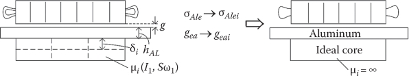
FIGURE 4.5 SLIM transverse cross section: equivalent cross section with ideal secondary back iron.

If the redistribution due to limited primary length is considered, the back-iron flux is

B t i \cdot δ i = B g 1 \cdot τ π \cdot (1 + k r d); k r d = (1 - 1.5) (4.28)

$B_{t i} \cdot δ_{i} = B_{g 1} \cdot \frac{τ}{π} \cdot (1 + k_{r d}); k_{r d} = (1 - 1.5) (4.28)$

with

δ i \approx 1 Re [ π 2 τ 2 + j \cdot μ i r o n \cdot ( σ i / k t i ) \cdot S \cdot ω 1 ] 1 / 2 (4.29)

$δ_{i} \approx \frac{1}{Re {[\frac{π^{2}}{τ^{2}} + j \cdot μ_{i r o n} \cdot (σ_{i} / k_{t i}) \cdot S \cdot ω_{1}]}^{1 / 2}} (4.29)$

The iron magnetization curve is accounted for B_ti = μ_iron · H_ti, by the B(H) curve on the secondary iron surface. Approximately (for low-S · G_e LIMs), the transverse edge effect coefficients (for Al and iron), k_trAL and k_ti, are (3.40) and (3.42):

k t r A L \approx 1 1 - tanh ( π τ \cdot a e ) ( π τ \cdot a e ) \cdot [ 1 + tanh ( π τ \cdot a e ) \cdot tanh π τ ( c - a e ) ] - 1 > 1 (4.30)

$k_{t r A L} \approx \frac{1}{1 - \frac{\tanh (\frac{π}{τ} \cdot a_{e})}{(\frac{π}{τ} \cdot a_{e})} \cdot {[1 + \tanh (\frac{π}{τ} \cdot a_{e}) \cdot \tanh \frac{π}{τ} (c - a_{e})]}^{- 1}} > 1 (4.30)$

k t i = 1 1 - tanh ( π τ \cdot a e i ) π τ \cdot a e i > 1; i = 1, 2, 3 (4.31)

$k_{t i} = \frac{1}{1 - \frac{\tanh (\frac{π}{τ} \cdot \frac{a_{e}}{i})}{\frac{π}{τ} \cdot \frac{a_{e}}{i}}} > 1; i = 1, 2, 3 (4.31)$

The equivalent goodness factor G_eALi becomes

G e A L i = μ 0 \cdot ω 1 \cdot τ 2 \cdot d A L π 2 \cdot g e a i \cdot σ e A l i (4.32)

$G_{e A L i} = \frac{μ_{0} \cdot ω_{1} \cdot τ^{2} \cdot d_{A L}}{π^{2} \cdot g_{e a i}} \cdot σ_{e A l i} (4.32)$

For reasonably small k_trAL, c = τ/π.

These expressions allow for SLIM circuit model following the same routine as for DLIM in the previous paragraph. But the secondary back-iron current density variation along penetration depth produces a leakage inductance L′₂_l, which may be approximated as (from eddy current theories [3])

L' 2 l \approx R ' 2 i S \cdot ω 1 = R ' 2 | S \cdot ω 1 | \cdot σ i \cdot δ i σ A L \cdot d A L \cdot k t r A l k t i \cdot k s k i n; | S \cdot ω 1 | > 2 π \times 1 [rad / s] (4.33)

${L^{'}}_{2 l} \approx \frac{{R^{'}}_{2 i}}{S \cdot ω_{1}} = \frac{{R^{'}}_{2}}{| S \cdot ω_{1} |} \cdot \frac{σ_{i} \cdot δ_{i}}{σ_{A L} \cdot d_{A L}} \cdot \frac{k_{t r A l}}{k_{t i}} \cdot k_{s k i n}; | S \cdot ω_{1} | > 2 π \times 1 [rad / s] (4.33)$

So the equivalent circuit for SLIMs has to be completed with the secondary back-iron leakage inductance (Figure 4.6).

As evident in Figure 4.6, the magnetization inductance L_m, secondary resistance R′₂, and the secondary iron leakage inductance L′₂_l (reduced to primary) depend on the primary mmf (or on linear current sheet J₁(I₁)) and on slip frequency S · ω₁. Moreover, the mechanical airgap g varies due to secondary (track) irregularities and on the primary on vehicle framing, light but inevitable, vibrations. To illustrate the magnitude of secondary solid iron influence on SLIM performance, let us consider the numerical results for a LIM with the data: τ = 0.084 m, 2a = 0.08 m, back-iron laminations count i = 3, number of poles 2p = 6, W₁(turns per phase) = 480, mechanical gap g + h_AL = 0.012 m, d_AL = 0.06 m, aluminum sheet overhang width 2c = 0.12 m, σ_AL = 3.5 × 10⁷ (Ω m)^–1, σ_i = 3.55 × 10⁶ (Ω m)^–1; stator slot depth h_s = 0.045 m, open slot width b_s = 0.009 m, y/τ = 5/6 (chorded coils).

Images

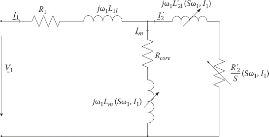
FIGURE 4.6 SLIM equivalent circuit.

The influence of iron on equivalent secondary conductivity accounts both for edge and for skin effects; this explains why σ_eALi/σ_AL < 1 and the presence of a minimum point (Figure 4.7a).

Images

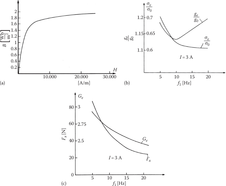
FIGURE 4.7 SLIM characteristics at standstill (a) iron magnetization curve, (b) equivalent airgap and electrical conductivity versus frequency, and (c) thrust and equivalent goodness factor versus frequency, at constant current. (After Boldea, I. and Nasar, S.A., Linear Motion Electromagnetic Systems, John Wiley, New York, 1985.)

Images

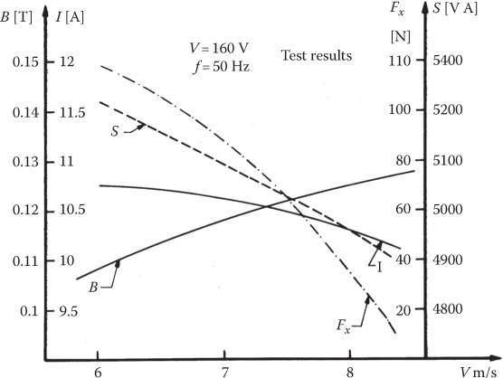
FIGURE 4.8 SLIM running test results (synchronous speed U_S = 2 · τ · f = 8.4 m/s). (After Boldea, I. and Nasar, S.A., Linear Motion Electromagnetic Systems, John Wiley, New York, 1985.)

A few remarks related to the results in Figures 4.7 and 4.8 are in order:

The airgap flux density of SLIMs for low-speed applications is rather low, and thus the thrust density is low, so are efficiency and power factor.
The case in point suggests to use, for same synchronous speed, a higher pole pitch τ = 2 · 0.084 = 0.168 m and 2p = 4 poles, to somehow alleviate the performance.
For short travels (a few meters), ladder secondary flat SLIM should be used for speeds below 10 m/s.

4.4 Flat SLIMs with Ladder Secondary

Low-speed flat SLIMs with ladder secondary (Figure 4.9) have been proposed (and used) for short travel (less than 3–4 m) applications (machining tables) for thrusts up to a few kN.

In such applications, the mechanical airgap may be as low as 1–2 mm. This is the whole magnetic airgap. For small airgap, at least the primary slots have to be semiclosed with openings (b_s₁) up to 4–6 mm, while the secondary ladder may be placed in a laminated core with slot openings b_s₂ of 2–3 mm. This way the Carter coefficient, due to double slotting, K_C <1.3–1.4 and the airgap fringing coefficient k_Fg ≈ 1.

Images

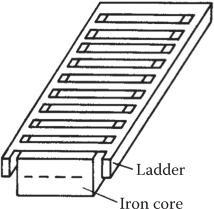
FIGURE 4.9 Ladder secondary of SLIM.

The airgap flux density at rated thrust may now be chosen as high as 0.65–0.7 T because the back iron in the secondary is laminated. The secondary ladder, made of aluminum, may be die casted in sections as for rotary IMs.

The parameters of the equivalent circuit have expressions similar to those of rotary cage rotor IMs:

R' 2 = 2 \cdot a \cdot ( W 1 \cdot k W 1 ) 2 p \cdot τ \cdot d A L \cdot b s 2 τ s 2 \cdot ( σ A L / k s k i n ) \cdot (1 + k e n d); k e n d = R r 2 \cdot R b \cdot sin 2 ( π \cdot p / N s 2 ) (4.34)

${R^{'}}_{2} = \frac{2 \cdot a \cdot {(W_{1} \cdot k_{W 1})}^{2}}{p \cdot τ \cdot d_{A L} \cdot \frac{b_{s 2}}{τ_{s 2}} \cdot (σ_{A L} / k_{s k i n})} \cdot (1 + k_{e n d}); k_{e n d} = \frac{R_{r}}{2 \cdot R_{b} \cdot \sin^{2} (π \cdot p / N_{s 2})} (4.34)$

k_end accounts for end-bars resistance in the ladder of secondary:

L' 2 l = 2 \cdot μ 0 \cdot 2 \cdot a \cdot 12 \cdot ( W 1 \cdot k w 1 ) 2 N s 2 \cdot (λ s 2 + λ d i f f 2 + λ e n d 2) (4.35)

${L^{'}}_{2 l} = 2 \cdot μ_{0} \cdot 2 \cdot a \cdot 12 \cdot \frac{{(W_{1} \cdot k_{w 1})}^{2}}{N_{s 2}} \cdot (λ_{s 2} + λ_{d i f f 2} + λ_{e n d 2}) (4.35)$

L m = 6 μ 0 π 2 \cdot ( W 1 \cdot k w 1 ) 2 \cdot τ \cdot 2 a g \cdot k c \cdot ( 1 + k s s ); λ s 2 \approx 1 - 2; λ d i f f 2 = 0.3 - 0.4; λ e n d = 0.7 - 1.5 \approx 0.6 (l e c 2 a) (4.36)

$L_{m} = \frac{6 μ_{0}}{π^{2}} \cdot \frac{{(W_{1} \cdot k_{w_{1}})}^{2} \cdot τ \cdot 2 a}{g \cdot k_{c} \cdot (1 + k_{s s})}; λ_{s 2} \approx 1 - 2; λ_{d i f f 2} = 0.3 - 0.4; λ_{e n d} = 0.7 - 1.5 \approx 0.6 (\frac{l_{e c}}{2 a}) (4.36)$

where

N_s₂ is the number of secondary slots per primary length

λ_s₂, λ_diff2, λ_end₂ are the geometric specific (nondimensional) permeances for secondary leakage field.

k_ss is the total (primary and secondary) core magnetic saturation coefficient (k_ss ≈ 0.3–0.6, in general)

b_s₂, τ_s₂ are the secondary slot opening and slot pitch (b_s₂/τ_s₂ ≈ 1/2)

R_r is the ladder end-bar section resistance

R_b is the secondary in-slot bar resistance

Let us consider a numerical example with τ = 0.1 m, 2p = 10, g = 1.5 mm, d_AL = 16 mm, b_s₂/τ_s₂ ≈ 1/2; k_end₂ = 0.3, 2a = 0.2 m, k_c = 1.3, k_skin = 1.25, σ_AL = 3.5 × 10⁷ (Ω m)^–1, k_ss = 0.1.

The goodness factor G_e, for U_s = 4 m/s (f₁ = 20 Hz) is

(G e) 20 Hz = μ 0 \cdot ω 1 \cdot τ 2 \cdot ( σ A L / k s k i n ) π 2 \cdot g \cdot k c \cdot d A L \cdot (b s τ s 1 + k e n d) = 1.256 \cdot 10 - 6 \cdot 2 π \cdot 20 \cdot 0.1 2 \cdot ( 3.5 \cdot 10 7 / 1.2 ) \cdot 1.6 \cdot 10 - 2 \cdot 1 2 π 2 \cdot 1.5 \cdot 1.3 \cdot 10 - 3 \cdot 1.1 \cdot 1.3 = 13.38

$\begin{array}{l} {(G_{e})}_{20 Hz} = \frac{μ_{0} \cdot ω_{1} \cdot τ^{2} \cdot (σ_{A L} / k_{s k i n})}{π^{2} \cdot g \cdot k_{c}} \cdot d_{A L} \cdot (\frac{\frac{b_{s}}{τ_{s}}}{1 + k_{e n d}}) \\ = \frac{1.256 \cdot 10^{- 6} \cdot 2 π \cdot 20 \cdot {0.1}^{2} \cdot (3.5 \cdot 10^{7} / 1.2) \cdot 1.6 \cdot 10^{- 2} \cdot \frac{1}{2}}{π^{2} \cdot 1.5 \cdot 1.3 \cdot 10^{- 3} \cdot 1.1 \cdot 1.3} = 13.38 \end{array}$

This rather high value would allow for maximum thrust (s_kG_e = 1), the slip s_k = 0.0747, to provide for a good power factor (above 0.75), besides a good efficiency (above 0.75); the rated slip may be even larger than S_k for S_mtedG_e = 1.3, for PWM vector control.

The ladder secondary thus seems capable of producing notable performance even for low-speed, low travel (3–4 m) and also for higher speeds (higher G_e ≤ G_e₀(2p)). The value of G_e = 13.38 < 20 (the optimum goodness factor for 2p = 10). Also, even at S = 0.1, the dynamic end effect is negligible as seen in Figure 4.1.

Note: As seen here, the dynamic end effect may be present even at small speeds (see in the previous example for 2p = 4, 6) – U = U_s*(1 – S) = 4*(1 – 0.1) = 3.6 m/s—if the goodness factor is high. In the earlier example, for 2p = 6, for example, it suffices to increase the airgap from 1.5 mm to 1.5* 10/6 = 2.5 mm to reduce G_e to G_e ≈ 8 and thus reduce the dynamic end effect to negligible influence, at the price of also reducing the conventional performance. In some small-speed applications, it may be thus preferable to allow for some dynamic longitudinal end effect for (2p = 4, 6) but still secure good performance due to higher G_e.

4.5 Tubular SLIM with Ladder Secondary

Tubular SLIM may be favored in short length (less than 2.5 m) travel applications due to zero net radial force between primary and secondary (for symmetric mover position in the airgap) and practically zero end connections of short-primary circular coils (Figure 4.10). Also, the stator is to be made of disk-shape laminations, with open slots (inevitably so) to cut the material and manufacturing costs; to reduce eddy current iron losses in the back iron (where the magnetic field goes perpendicular to lamination plane), thin radial slits are cut in the back-iron laminations (Figure 4.10b); the same is valid for the secondary core; the secondary ladder is made of aluminum rings or short-circuited circular-shape coils in open slots; the slot opening should not surpass 3 airgap lengths in the secondary and 4–5 airgaps in the primary, to limit Carter coefficient. This way, with an airgap of 1–1.5 mm, good results are expected in terms of performance/cost, with respect to tubular linear permanent magnet synchronous motors, which represent such a strong competition that the Al-on-iron secondary was discarded here for tubular SLIMs (Figure 4.10). Only the ladder secondary is considered.

Images

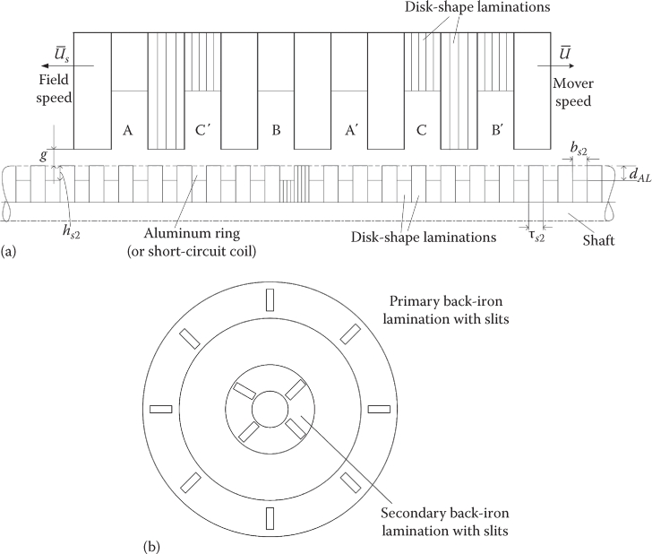
FIGURE 4.10 Tubular SLIM with ladder secondary: (a) longitudinal cross section, (b) back-iron laminations with slits.

Note: For very short travels (less than 0.4–0.5 m) and long (fix) primary with short mover secondary, to reduce the mover weight and avoid a flexible power cable, a dual airgap structure, with an aluminum cylinder with embedded Somaloy inserts (as teeth), which reduces the magnetic airgap to the mechanical dual one, is proposed. As linear PM synchronous motors represent a strong contender for such applications, this solution is not pursued here further.

The tubular SLIMs with ladder secondary parameters have expressions similar to flat SLIMs, but the primary and secondary coils are circular and only slot and differential leakage inductances exist; the stack width now becomes π · D_is (D_is, secondary outer diameter); so no secondary transverse edge effect occurs; skin effect in the secondary remains present and is treated as for rotary cage rotor IMs:

R 1 t = ρ c o π \cdot D a v 1 \cdot j c o r \cdot W 2 1 I 1 r \cdot w 1 = k R 1 t \cdot W 21; X 1 l = 2 μ 0 \cdot π \cdot D a v 1 p \cdot q \cdot (λ s l o t 1 + λ d i f f 1) \cdot W 21 = k 1 l t \cdot W 21 L m = 6 μ 0 π 2 \cdot ( W 1 \cdot k W 1 ) \cdot τ \cdot π \cdot D i s p \cdot g \cdot k c L' 2 l = 2 μ 0 \cdot π \cdot D a v 2 \cdot 12 \cdot ( W 1 \cdot k W 1 ) 2 N s 2 \cdot (λ s 2 + λ d i f f 2) = k 2 l t \cdot ω 21 R' 2 = ρ A L π \cdot D a v 2 \cdot 12 \cdot ( W 1 \cdot k W 1 ) 2 A r i n g \cdot N s 2 = k R 2 t \cdot W 21 = k L m \cdot W 21; A r i n g = b s 2 \cdot h s 2 \cdot k f i l l 2 (4.37)

$\begin{matrix} R_{1 t} = ρ_{c o} \frac{π \cdot D_{a v 1} \cdot j_{c o r} \cdot W_{1}^{2}}{I_{1 r} \cdot w_{1}} = k_{R 1 t} \cdot W_{1}^{2}; X_{1 l} = \frac{2 μ_{0} \cdot π \cdot D_{a v 1}}{p \cdot q} \cdot (λ_{s l o t 1} + λ_{d i f f 1}) \cdot W_{1}^{2} = k_{1 l t} \cdot W_{1}^{2} \\ L_{m} = \frac{6 μ_{0}}{π^{2}} \cdot \frac{(W_{1} \cdot k_{W 1}) \cdot τ \cdot π \cdot D_{i s}}{p \cdot g \cdot k_{c}} \\ {L^{'}}_{2 l} = \frac{2 μ_{0} \cdot π \cdot D_{a v 2} \cdot 12 \cdot {(W_{1} \cdot k_{W 1})}^{2}}{N_{s 2}} \cdot (λ_{s 2} + λ_{d i f f 2}) = k_{2 l t} \cdot ω_{1}^{2} \\ {R^{'}}_{2} = ρ_{A L} \frac{π \cdot D_{a v 2} \cdot 12 \cdot {(W_{1} \cdot k_{W 1})}^{2}}{A_{r i n g} \cdot N_{s 2}} = k_{R 2 t} \cdot W_{1}^{2} = k_{L m} \cdot W_{1}^{2}; A_{r i n g} = b_{s 2} \cdot h_{s 2} \cdot k_{f i l l 2} \end{matrix} (4.37)$

With the given rated phase mmf W₁ · I₁_n and rated current density j_cor, all parameters of the equivalent circuit (as for flat LIMs) are proportional to the number of turns/phase squared. This peculiarity will help notably in the design process as evident in the next chapter.

Also, the reasonably small airgap (1–1.5 mm) for short travel (0.3–1.5 m), though larger than that in rotary IMs, provides for acceptable performance/cost and reliability in applications where PMs are to be avoided.

4.6 Circuit Models of High-Speed (High Goodness Factor) SLIMs

By high-speed LIMs, we mean LIMs where dynamic end effects have to be considered; as already explained in this chapter, the dynamic end effect can occur in ladder secondary LIMs of small airgap (short travels) even at low speeds (4–5 m/s), at large goodness factor (G_e > 8) values, for a small number of poles (2p = 2, 4). So we might as well use the term high goodness factor or large dynamic end effect LIMs, instead of high-speed LIMs.

Accounting for dynamic end effect in the circuit model would mean introducing its influence on the conventional circuit parameters and adding new ones.

The first attempt [4] relied on the idea that the end effect reduces the thrust and consequently reduces the emf k_e times. This effect may be translated into an additional parallel term in the equivalent circuit Z_e:

Z ¯ ¯ ¯ e = j \cdot X m \cdot ( R ' 2 / s + j \cdot X ' 2 l ) R ' 2 s + j \cdot ( X m + X ' 2 l ) \cdot 1 - k e k e (4.38)

${\underline{Z}}_{e} = \frac{j \cdot X_{m} \cdot ({R^{'}}_{2} / s + j \cdot {X^{'}}_{2 l})}{\frac{{R^{'}}_{2}}{s} + j \cdot (X_{m} + {X^{'}}_{2 l})} \cdot \frac{1 - k_{e}}{k_{e}} (4.38)$

with

E s e \approx E m s \cdot (1 - k e); E m s = X m \cdot I m

$E_{s e} \approx E_{m s} \cdot (1 - k_{e}); E_{m s} = X_{m} \cdot I_{m}$

k e = k w e 1 k w 1 π \cdot τ e τ 2 γ 2 2 r + ( π τ e ) 2 \cdot f (δ) \cdot e - p \cdot τ e | γ 2 r | \cdot sinh ( p \cdot τ e \cdot γ 2 r ) p \cdot sinh ( τ e \cdot γ 2 r ); f (δ) \approx γ 2 r \cdot sin δ + π τ e \cdot cos δ

$k_{e} = \frac{k_{w e 1}}{k_{w 1}} \frac{\frac{π \cdot τ_{e}}{τ^{2}}}{γ_{2 r}^{2} + {(\frac{π}{τ_{e}})}^{2}} \cdot f (δ) \cdot e^{- p \cdot τ_{e} | γ_{2 r} |} \cdot \frac{\sinh (p \cdot τ_{e} \cdot γ_{2 r})}{p \cdot \sinh (τ_{e} \cdot γ_{2 r})}; f (δ) \approx γ_{2 r} \cdot \sin δ + \frac{π}{τ_{e}} \cdot \cos δ$

δ = δ 0 + c 1 \cdot U; δ 0 \approx 3 π 4

$δ = δ_{0} + c_{1} \cdot U; δ_{0} \approx \frac{3 π}{4}$

k w e 1 = sin ( τ τ e \cdot π 6 ) q 1 \cdot sin ( τ τ e \cdot π 6 \cdot q 1 ) \cdot sin (τ τ e \cdot π 6 \cdot y τ); γ 2 r from (4.2)

$k_{w e 1} = \frac{\sin (\frac{τ}{τ_{e}} \cdot \frac{π}{6})}{q_{1} \cdot \sin (\frac{τ}{τ_{e}} \cdot \frac{π}{6 \cdot q_{1}})} \cdot \sin (\frac{τ}{τ_{e}} \cdot \frac{π}{6} \cdot \frac{y}{τ}); γ_{2 r} from (4.2)$

with k_we₁, τ_e winding factor and pole pitch for the exit end wave (3.67); U is the LIM speed and c₁ is [4]

C 1 \approx 1 U s max \cdot tan (π \cdot τ e τ) U = U s max / 2 (4.39)

$C_{1} \approx \frac{1}{U_{s \max}} \cdot \tan {(\frac{π \cdot τ_{e}}{τ})}_{U = U_{s \max / 2}} (4.39)$

The equivalent circuit in Figure 4.11 has been checked against two LIMs one of medium speed and one of high speed, with good agreement in terms of thrust versus speed for given phase current (Figures 4.12 and 4.13) [4].

As the verifications of active, reactive powers and secondary losses agreement of equivalent circuit in Figure 4.11 with field theory results (Chapter 3) have not been performed, subsequently, starting from the same idea of emf reduction by end effect, modifications in all components of the standard circuit model have also been added (Figure 4.14) [5].

The end effect impedance Z_e in Figure 4.14 [5] is the same as in Figure 4.11 [4] but, in addition, the coefficients k_xe and k_Re are calculated from the single dimensional field theory (see Chapter 3) by airgap reactive and active secondary power balance. The thrust and power factor agreement of this circuit with experiments on a 6 pole LIM with τ = 0.2868 m, aluminum (6 mm) on iron secondary, with 10 mm airgap, have proved very good at synchronous speeds of up to 28.68 m/s (140 kW SLIM for urban transportation).

Images

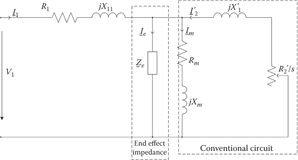
FIGURE 4.11 LIM equivalent circuit with simplified end effect impedance Z_e.

Images

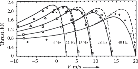
FIGURE 4.12 Thrust/speed curves for constant current: theory versus experiments—CIGGT-LIM. (After Gieras, J.F. et al., IEEE Trans., EC-2(1), 152, 1987.)

Images

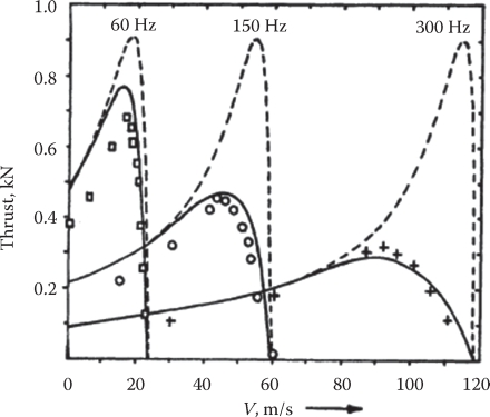
FIGURE 4.13 Thrust/speed curves for constant current: GEC–LIM. (After Gieras, J.F. et al., IEEE Trans., EC-2(1), 152, 1987.)

Images

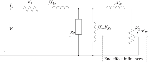
FIGURE 4.14 More complete equivalent circuit of LIM with end effect. (After Cabral, C.M.A.R., Analysis of LIMs using new longitudinal end effect factors, Record of LDIA-2003, Birmingham, U.K., pp. 291–294, 2003.)

An experimentally based method that measures the LIM equivalent impedance at a few representative speeds, slip frequencies, and primary currents may also be used to identify the equivalent circuit curve fitting, to estimate the equivalent circuit parameters.

Both constant current and constant voltage (with variable frequency) tests may be performed for the scope.

The equivalent circuit models so far have integrated rather well all end effect influences, but at the price of variable parameters (with speed and current); in essence, only L_m and R′₂ vary with speed and current; and an additional end effect impedance (resistance, even) Z_e(k_e) is added; k_e is variable with speed. Even linear variations (L_m and R′₂ increase with speed) would suffice at a first approximation to be used in circuit models for transients and control.

4.7 Low-Speed Lim Transients and Control

The circuit models of low-speed LIMs, which are in general single sided, with aluminum-iron secondary for longer travel (above 3–4 m), have parameters variable with slip frequency (due to skin and/or edge effects) and magnetization current I_m (or primary current) due to magnetic saturation.

In short, the LIM is like a rotary equivalent induction machine with variable parameters. Magnetic saturation or airgap influence on magnetization inductance may be (and is) handled by L_m(I_m) to investigate transients by the d–q model, which may be used for low-speed (low end effect) LIMs, with small adaptations.

Moreover, the secondary resistance variations with slip frequency may be small as the slip frequency is controlled in inverter-fed (all) LIM drives.

But the presence of solid back iron behind the aluminum sheet of LIM secondary leads to a variation of R′₂ with I_m also: this is unknown in regular cage rotor rotary IMs (but known to solid rotor high-speed rotary IMs).

Let us consider R′₂ (I_m) only in such SLIMs.

Now it becomes evident that we may use the d–q model for low-speed LIM transients and control.

4.7.1 Space–Phasor (DQ) Model

The rotary IM space–phasor model can be adapted rather easily for low-speed LIMs; in general coordinates,

V ¯ ¯ ¯ 1 = R 1 \cdot i ¯ 1 + d ψ ¯ ¯ 1 d t + j ω b λ ¯ 1; V ¯ ¯ ¯ 1 = V d + j V q; i ¯ 1 = j i q; ω b = ω 1 V' 2 = 0 = R' 2 \cdot i ¯' 2 + d ψ ¯ ¯ ' 2 d t + j \cdot (ω b - ω r) \cdot ψ ¯ ¯' 2; i' 2 = i D + j i Q F x = - 3 2 \cdot π τ \cdot (ψ ¯ ¯ 1 i ¯ * 1); ψ ¯ ¯ 1 = L 1 \cdot i 1 + L m \cdot i' 2; ψ ¯ ¯' 2 = L' 2 \cdot i' 2 + L m \cdot i 1 L 1 = L 1 l + L m; L' 2 = L' 2 l + L m; i m = i 1 + i' 2; ω 1 = U s \cdot π τ (4.40)

$\begin{array}{l} {\bar{V}}_{1} = R_{1} \cdot {\bar{i}}_{1} + \frac{d {\bar{ψ}}_{1}}{d t} + j ω_{b} {\bar{λ}}_{1}; {\bar{V}}_{1} = V_{d} + j V_{q}; {\bar{i}}_{1} = j i_{q}; ω_{b} = ω_{1} \\ {V^{'}}_{2} = 0 = {R^{'}}_{2} \cdot {\bar{i}}^{'}_{2} + \frac{d {\bar{ψ}}^{'}_{2}}{d t} + j \cdot (ω_{b} - ω_{r}) \cdot {\bar{ψ}}^{'}_{2}; {i^{'}}_{2} = i_{D} + j i_{Q} \\ F_{x} = \frac{- 3}{2} \cdot \frac{π}{τ} \cdot ({\bar{ψ}}_{1} {\bar{i}}_{1}^{*}); {\bar{ψ}}_{1} = L_{1} \cdot i_{1} + L_{m} \cdot {i^{'}}_{2}; {\bar{ψ}}^{'}_{2} = {L^{'}}_{2} \cdot {i^{'}}_{2} + L_{m} \cdot i_{1} \\ L_{1} = L_{1 l} + L_{m}; {L^{'}}_{2} = {L^{'}}_{2 l} + L_{m}; i_{m} = i_{1} + {i^{'}}_{2}; ω_{1} = \frac{U_{s} \cdot π}{τ} \end{array} (4.40)$

F n a \approx 3 2 \cdot L m \cdot i 2 m g e; θ = \int ω 1 d t = - \int (S \cdot ω 1 + ω r) d t (4.41)

$F_{n a} \approx \frac{3}{2} \cdot \frac{L_{m} \cdot i_{m}^{2}}{g_{e}}; θ = \int ω_{1} d t = - \int (S \cdot ω_{1} + ω_{r}) d t (4.41)$

A few remarks are in order:

The equations are similar to those of single-cage rotary IMs (in the absence of end effects).
The thrust, F_x, equation has the sign (–) because the primary is the mover.
ω_b is the speed of the reference system ω_b = ω₁ for synchronous coordinates.
The sign (–) in the reference system angle θ_b is due to the fact that the primary is the mover.
The normal attraction force (total normal force for cage secondary LIM) F_na is obtained here as the derivative of magnetic energy in the airgap with respect to airgap g_e.
Apparently, the number of pole pairs p does not occur in thrust F_x, but, in fact, it is involved implicitly by the flux ${\bar{Ψ}}_{1}$ expression. The space–phasor diagrams for steady state (d/dt = 0) in synchronous coordinates (ω_b = ω₁) are shown in Figure 4.15 for motoring and generating (regenerative braking).

Images

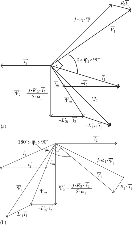
FIGURE 4.15 The space–phasor diagram of low-speed LIMs for steady state: (a) motoring, (b) generating.

The investigation of transients may be approached directly by Equation 4.40, say, in synchronous coordinates ω_b = ω₁ with the d/dt replaced by s (Laplace operator):

$\begin{array}{l} V_{1} (s) = R_{1} \cdot i_{1} (s) + s \cdot Ψ_{1} (s) + j \cdot ω_{1} \cdot Ψ_{1} (s) \\ 0 = {R^{'}}_{2} \cdot {i^{'}}_{2} (s) + s \cdot {Ψ^{'}}_{2} (s) + j \cdot ω_{1} \cdot {Ψ^{'}}_{2} (s) \end{array} (4.42)$

Apparently, we do have four variables and two equations, but the flux/current relationships reduce the number of complex variables to two. To include the wound secondary case V′₂ ≠ 0 in (4.40) and for more generality we adopt this case.

Three types of controls seem practical:

I₁ – f₁ (scalar control)
Secondary (“rotor”) vector control $({\bar{Ψ}}^{'}_{2}, {\bar{i}}_{1})$ : FOC
Direct thrust and flux control (F_x, Ψ₁): DTFC

The earlier control methods introduce constraints and thus reduce the order of the system (4.41), which still needs the motion equations:

$m s U = m \frac{d U}{d t} = F_{x} - F_{l o a d}; s \cdot θ_{b} = \frac{d θ_{b}}{d t} = - S \cdot ω_{1} - \frac{U}{τ} \cdot π (4.43)$

Also, the primary voltage vector $\bar{V}$ is

${\bar{V}}_{1} = \frac{2}{3} \cdot (V_{a} + V_{b} \cdot e^{j \frac{2 π}{3}} + V_{c} \cdot e - j \frac{2 π}{3}) \cdot e^{- j θ_{b}} (4.44)$

For constant speed (U = ct) transients equations (4.41) suffice and, after eliminating the currents $\bar{i}$ and ${\bar{i}}^{'}$ , we are left with two equations with primary and secondary flux vectors as variables [6]:

$\begin{matrix} {τ^{'}}_{s} \cdot s \cdot Ψ_{1} + (1 + j \cdot ω_{1} \cdot {τ^{'}}_{s}) \cdot Ψ_{1} = {τ^{'}}_{s} \cdot V_{1} + k_{r} \cdot {Ψ^{'}}_{2}; τ_{s} = \frac{L_{1}}{R_{1}} \\ {τ^{'}}_{r} \cdot s \cdot {Ψ^{'}}_{2} + (1 + j \cdot s \cdot ω_{1} \cdot {τ^{'}}_{r}) \cdot {Ψ^{'}}_{2} = {τ^{'}}_{r} \cdot {V^{'}}_{2} + k_{s} \cdot Ψ_{1}; τ_{r} = \frac{{L^{'}}_{2}}{{R^{'}}_{2}} \\ k_{s} = \frac{L_{m}}{L_{1}}; k_{r} = \frac{L_{m}}{{L^{'}}_{2}}; {τ^{'}}_{s} = τ_{s} \cdot σ; {τ^{'}}_{r} = τ_{r} = τ_{r} \cdot σ; σ = 1 - \frac{L_{m}^{2}}{{L^{'}}_{2} \times L_{1}} \end{matrix} (4.45)$

It is now evident that the eigen values of the system (4.45) are obtained by solving the characteristic equation:

$\begin{matrix} 1 + (s + j \cdot ω_{1}) \cdot {τ^{'}}_{s} & - k_{r} \\ - k_{s} & 1 + (s + j \cdot S \cdot ω_{1}) \cdot {τ^{'}}_{r} \end{matrix} | = 0 (4.46)$

It may be proved that the real part of γ_1,2 eigen values is negative, for the stable part of the mechanical curve F_x(U), for given V₁ and V′₂ = 0 as known from the critical slip frequency of rotary IMs:

${(S \cdot ω_{1})}_{k} \approx \frac{{R^{'}}_{2}}{L_{1 l} + {L^{'}}_{2 l}} (4.47)$

Images

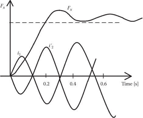
FIGURE 4.16 Typical sudden ac symmetrical input at standstill, from zero current.

In essence, however, there are two complex eigen values and two rather fast time constants for LIM transients τ′_s and τ′_r; one inflicted by the primary $({τ^{'}}_{s})$ and the other by the secondary $({τ^{'}}_{r})$ . As the solutions of (4.46) are analytical, the LIM transients at constant speed are straightforward. Also, as the LIM mover mass is rather large, the mechanical transients are notably slower than electromagnetic transients, so that they can be solved separately by inserting the flux and current instantaneous values in the thrust expression present in the motion equation.

A typical qualitative response, at standstill, with sudden sinusoidal voltages (of given frequency) application and zero initial current, is shown in Figure 4.16.

The sum of two currents i₁ + i′₂ is the magnetization current i_m, and the thrust builds up after some time because it takes time to install the magnetic flux in the machine, to interact with current for thrust production.

Much faster thrust response is obtained with the flux already installed in the machine, even if a single voltage vector is preapplied to produce a dc field (with fixed position) in the LIM, before starting.

4.8 Control of Low-Speed LIMs

As already stated in this chapter, scalar (SC), vector (FOC), and direct torque and flux control (DTFC) seem [6] the most practical solutions.

Let us start with scalar I₁ - Sf₁ close-loop control.

4.8.1 Scalar I₁ – Sf₁ Close-Loop Control

As shown in the circuit model of LIMs, the thrust is

$F_{x} = \frac{3 \cdot I_{1}^{2} \cdot {R^{'}}_{2}}{2 \cdot τ \cdot f_{1} \cdot S \cdot (1 + {(\frac{1}{S \cdot G_{e}})}^{2})}; G_{e} \approx ω_{1} \cdot \frac{L_{m}}{{R^{'}}_{2}} (4.48)$

with current and slip frequency as controlled variables, a simple control strategy may be developed with and without a speed control loop.

Images

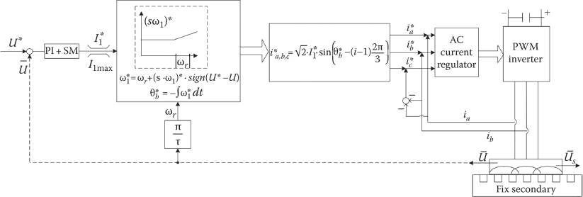
FIGURE 4.17 I–f close-loop control of LIMs.

The maximum thrust/current is obtained for

${(S \cdot ω_{1})}_{k} = \frac{{R^{'}}_{2}}{L_{m}} (4.49)$

The slip frequency may be kept constant, up to base speed obtained at full voltage, for sustained full load and then increased a little for flux weakening.

Increasing S · ω₁ over (S · ω₁)_k means reducing the efficiency, but still allowing higher speed/thrust envelope.

A generic block diagram is shown in Figure 4.17.

A few notes on Figure 4.17 are in order:

Motoring and regenerative braking may be provided and the slip frequency is feed forwarded.
The speed controller (illustrated here by a PI plus sliding mode implementation—for robustness) outputs the stator phase current RMS value which is limited, for protection.
With measured LIM speed, the primary frequency $ω_{1}^{*}$ is feed forwarded via the current angle $θ_{b}^{*}$ for the three reference currents $i_{a}^{*}, i_{b}^{*}, i_{c}^{*}$ .
AC current regulators (individual or current vector error or predictive regulators) are used to control the PWM inverter.
An outer position close loop may be added if position control action is targeted.
Though called scalar control, the scheme in Figure 4.17 is almost equivalent with indirect current vector control (used for rotary IMs).
As the parameters (L_m, R₂) may vary with current I₁ and slip frequency, Sω₁, the control is not fully robust, but the PI + SM speed regulator compensates for this drawback notably, despite the apparent simplicity of the control scheme.

4.8.2 Vector Control of Low-Speed LIMs

Vector control means independent flux and thrust control in LIMs. It may be primary flux ${\bar{Ψ}}_{1}$ , airgap flux ${\bar{Ψ}}_{m}$ , or secondary flux ${\bar{Ψ}}^{'}_{2}$ . The implementation of vector control (FOC) relates to separate control of the primary-flux current i_M and thrust current i_T components in synchronous coordinates (ω_b = ω₁; dc in steady state).

While FOC can be performed for all the defined fluxes, only with constant secondary flux Ψ′₂ amplitude the thrust/speed curves are linear; that is ideal for control purposes (as in dc brush PM motors!). So, returning to the space–phasor model (4.32 through 4.42), we may eliminate secondary current I′₂ and primary flux ${\bar{Ψ}}_{1}$ to obtain

${\bar{V}}_{1} (R_{1} + (S + j \cdot ω_{1}) \cdot L_{S C}) \cdot {\bar{i}}_{1} + (s + j \cdot ω_{1}) \cdot \frac{L_{m}}{{L^{'}}_{2}} \cdot {Ψ^{'}}_{2} (4.50)$

If the secondary flux is kept constant, in synchronous coordinates, it means s Ψ′₂ = 0 in the two equations mentioned previously.

So the system becomes a first-order one:

$\begin{matrix} 0 = {R^{'}}_{2} \cdot {i^{'}}_{2} (s) + j \cdot S \cdot ω_{1} \cdot {Ψ^{'}}_{2} (s) \\ {\bar{V}}_{1} = (R_{1} + (s + j \cdot ω_{1}) \cdot L_{s c}) \cdot {\bar{i}}_{1} + j \cdot ω_{1} \cdot \frac{L_{m}}{{L^{'}}_{2}} \cdot {\bar{Ψ}}^{'}_{2} \\ {\bar{i}}_{s} = \frac{{\bar{Ψ^{'}}}_{2}}{L_{m}} + j \cdot S \cdot ω_{1} \frac{{\bar{Ψ^{'}}}_{2}}{L_{m}} \cdot \frac{{L^{'}}_{2}}{{R^{'}}_{2}} = i_{M} + j \cdot t_{T} \\ i_{M} = \frac{{\bar{Ψ^{'}}}_{2}}{L_{m}}; i_{T} = i_{M} \cdot S \cdot ω_{1} \cdot \frac{{L^{'}}_{2}}{{R^{'}}_{2}} \end{matrix} (4.51)$

Also,

${\bar{Ψ}}_{1} = L_{1} \cdot i_{M} + j \cdot L_{s c} \cdot i_{T} (4.52)$

Finally, the thrust is simply

$F_{x} = \frac{- 3}{2} \cdot \frac{π}{τ} \cdot Imag ({\bar{Ψ}}_{1} * {\bar{i}}_{1}) = \frac{- 3}{2} \cdot \frac{π}{τ} \cdot (L_{1} - L_{s c}) \cdot I_{M} \cdot I_{T} (4.53)$

where

$L_{s c} = L_{1} - \frac{L_{m}^{2}}{{L^{'}}_{2}} (4.54)$

With (4.51), F_x becomes

$F_{x} = \frac{- 3}{2} \cdot \frac{π}{τ} \cdot (L_{1} - L_{s c}) \cdot {(\frac{{\bar{Ψ}}^{'}_{2}}{L_{m}})}^{2} \cdot \frac{{L^{'}}_{2}}{{R^{'}}_{2}} \cdot S \cdot ω_{1} = \frac{- 3}{2} \cdot \frac{π}{τ} \cdot \frac{({Ψ^{'}}_{2})}{{R^{'}}_{2}} \cdot (ω_{1} - ω_{r}) (4.55)$

Equation 4.55 suggests a straight-line F_x(U) curve for constant secondary flux amplitude Ψ′₂. By varying the frequency at constant Ψ′₂, a family of F_x(U) straight lines are obtained (Figure 4.18).

Now the voltage vector components under steady state are

$\begin{array}{l} V_{M} = R_{1} \cdot I_{M} - ω_{1} \cdot L_{s c} \cdot I_{T} \\ V_{T} = R_{1} \cdot I_{T} + ω_{1} \cdot L_{1} \cdot I_{M} \end{array} (4.56)$

Images

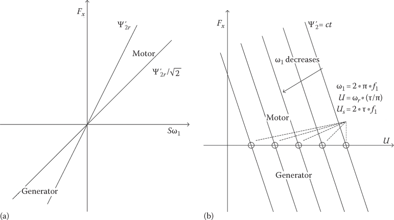
FIGURE 4.18 Mechanical characteristics at constant secondary flux Ψ′₂: (a) F_x(Sω₁), (b) F_x(U).

Example 4.1

Let us consider a SLIM with the data: R₁ = 1 ω, R₂ = 2 ω, Ψ′₂ = 1 w b, L_m = 0.1 H, L₁_l = 0.03 H, L′₂₁ = 0 01H, τ = 0, 1 m, which works at f₂ = S · f₁ = 4 Hz, at a primary frequency of 40 Hz.

Calculate:

The speed
IM, IT, and thrust
VM, V_T, V₁ (RMS per phase), I₁ (RMS per phase), the efficiency and power factor (η₁, cos φ₁)

Solution

The synchronous speed U_s = 2 · τ · f₁ = 2 · 0.1 · 40 = 8 m/s, while the LIM speed U = 2 · τ · (f₁ – f₂) = 2 · 0.1 · (40 – 4) = 7.2 m/s.
From (4.51), $\begin{array}{l} I_{M} & = & \frac{{\bar{Ψ}}^{'}_{2}}{L_{m}} = \frac{1}{0.1} = 10 A, I_{T} = i_{M} \cdot \frac{{L^{'}}_{2}}{{R^{'}}_{2}} \cdot S \cdot ω_{1} \\ = & 10 \cdot \frac{0.11}{2} \cdot 2 \cdot π \cdot 4 = 13.81 A({L^{'}}_{2} = L_{m} + {L^{'}}_{2 I} =0 .1+0 .1=0 .11H) \end{array}$

The short circuit inductance L_sc (4.54) is L_sc = L₁ – L²_m/L′₂ = 0.13 – 0.1²/0.11 = 0.0391H. So the thrust (4.53) is

$F_{x} = \frac{- 3}{2} \cdot \frac{π}{τ} \cdot (L_{1} - L_{s c}) \cdot I_{M} \cdot I_{T} = - \frac{π}{0.1} \cdot \frac{3}{2} \cdot (0.13 - 0.0391) \cdot 10 \cdot 13.816 = - 591.5 N$
V_M and V_T from (4.56) are

$\begin{array}{l} V_{M} = 1 \cdot 10 - 2 \cdot π \cdot 40 \cdot 0.0394 \cdot 13.816 = - 126 V \\ V_{T} = 1 \cdot 13.816 + 2 \cdot π \cdot 40 \cdot 0.13 \cdot 10 = 340.37 V \end{array}$

$\begin{array}{l} V_{1} = \sqrt{\frac{V_{M}^{2} + V_{T}^{2}}{2}} = 256 V (RM S perphase) \\ I_{1} = \sqrt{\frac{I_{M}^{2} + I_{T}^{2}}{2}} = 12.06 A (RM S perphase) \end{array}$

The η₁ cos φ₁ (with zero core losses and mechanical losses) is

$η_{1} \cos φ_{1} = \frac{F_{X} \cdot U}{3 \cdot V_{1} \cdot I_{1}} = \frac{591.5 \times 7.2}{3 \times 256 \times 12.06} = 0.4598$

And efficiency η₁:

$\begin{matrix} η_{1} = \frac{F_{x} \cdot U}{F_{x} \cdot U + 3 \cdot {R^{'}}_{2} \cdot {I^{'}}_{2}^{2} + 3 \cdot R_{1} \cdot I_{1}^{2}} \\ {I^{'}}_{2} \sqrt{2} = \frac{- L_{m} \cdot I_{T}}{{L^{'}}_{2}} ({\bar{Ψ}}^{'}_{2 T} = 0) and thus {I^{'}}_{2} = \frac{0.1}{0.11} \cdot \frac{13.816}{\sqrt{2}} = 8.907 A (RM S/phase) . \end{matrix}$

So

$η_{1} = \frac{591.5 \cdot 7.2}{591.5 \cdot 7.2 + 3 \cdot 2 \cdot {8.907}^{2} + 3 \cdot 1 \cdot {13.816}^{2}} = 0.8$

Finally, the power factor cos φ₁ = 0.4598/0.8 = 0.573.

Note: The results show acceptable efficiency but rather low power factor; only with a cage secondary and rather small airgap (1–1.5 mm), power factor values above 0.7 can be hoped for.

As for a vector control (FOC), there are quite a few options; we will illustrate an indirect combined current and voltage vector control as it is rather robust, except for very low speeds (Figure 4.19). For another FOC of LIMs, see Ref. [7].

Images

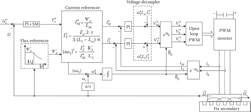
FIGURE 4.19 Field-oriented LIM control.

The control block in Figure 4.19 is characterized by

A secondary-flux referencer where the secondary-flux amplitude stays constant up to base speed, and then, for flux weakening, it decreases with speed
A current referencer that calculates online flux and thrust current components i_M and i_T in synchronous coordinates
A slip frequency (Sω₁) and rotation angle θ*_b online calculator
PI dc current controllers
A voltage decoupler
An open-loop PWM method that “copies” the sinusoidal symmetric reference voltages $V_{a}^{*}, V_{b}^{*}, V_{c}^{*}$ in the inverter

4.8.3 Sensorless Direct Thrust and Flux Control of Low-Speed LIMs

In an attempt to condense the presentation of an implemented sensorless direct thrust and flux control (DTFC) system for low-speed LIMs, a motion-sensorless solution is presented [7].

DTFC is in fact the equivalent of a direct primary-flux-oriented combined vector current and voltage control system. As primary-flux orientation control is targeted, the F_x(U) curves are not any more straight lines, but they show up for voltage-source supply, those known maximums (for motoring and generating). To secure stability, the slip frequency has to be limited:

${(S \cdot ω_{1})}_{Ψ_{s}} \leq \frac{{R^{'}}_{2}}{L_{s c}} (4.57)$

In DTFC, the primary-flux amplitude and thrust errors (ΔΨ₁, ΔF_x), corroborated with the position of the primary-flux vector in one of the six 60° wide sectors, starting with the magnetic axis of phase A, lead to a planned combination of neighboring nonzero and zero voltage vectors in the inverter. In effect, we provoke a primary-flux vector accelerating or decelerating (for motoring and generating) and the adjustment of flux amplitude.

So there should be two internal closed loops, one for primary flux and one for thrust, besides the speed control loop that outputs the reference thrust F*_x.

The primary-flux amplitude may be constant up to base speed and then decrease with speed to allow additional speed range for maximum inverter voltage V_max.

DTFC presupposes, then, a primary-flux observer and a thrust estimator.

Speed sensorless control requires a speed observer additionally.

A primary-flux observer based on the primary voltage model is represented by the equation

$\frac{d {\overset{⌢}{Ψ}}_{1}}{d t} = - R_{1} \cdot {\bar{i}}_{1} + {\bar{V}}_{1} + (k_{p} + k_{i} / S) \cdot sgn ({\bar{i}}_{1} - {\overset{⌢}{i}}_{1}) (4.58)$

$\overset{⌢}{i}$ is the estimated stator current vector; for its estimation, we first need an estimation of secondary flux:

$\frac{d {\overset{⌢}{Ψ}}_{2 r}}{d t} + \frac{{R^{'}}_{2}}{L_{1 l}} \cdot \frac{L_{1}}{L_{m}} \cdot {\overset{⌢}{Ψ}}^{'}_{2 r} = \frac{{R^{'}}_{2}}{L_{1 l}} \cdot {\overset{⌢}{Ψ}}_{1 r} + k_{2} \cdot sgn (i_{1} - {\overset{⌢}{i}}_{1}) (4.59)$

In (4.59) for simplification L′₂_l = 0, which is a realistic assumption.

The secondary flux in primary coordinates ${\overset{⌢}{Ψ}}^{'}_{2}$ is

${\hat{Ψ}}^{'}_{2} = {\overset{⌢}{Ψ}}_{1} - L_{1 l} \cdot {\bar{i}}_{1}; {\overset{⌢}{θ}}_{Ψ_{2}} = \tan^{- 1} {\overset{⌢}{Ψ}}_{2β} / {\overset{⌢}{Ψ}}_{2 α} (4.60)$

θ_Ψ2 is the estimated position of the secondary flux with respect to primary. The adopted sliding mode functional $S_{S} = sgn (i_{1} - {\overset{⌢}{i}}_{1})$ .

To reduce the chattering, the sgn function is replaced by sat(x):

$sat (x) = {\begin{array}{l} sgn (x), & for | x | > h \\ x / h, & for | x | \leq h \end{array} (4.61)$

The block diagram for the primary- and secondary-flux observers based on these equations is shown in Figure 4.20.

The thrust estimation is

${\overset{⌢}{F}}_{x} = - \frac{π}{τ} \cdot \frac{3}{2} \cdot Imag ({\overset{⌢}{Ψ}}_{1} * i_{1}) = \frac{π}{τ} \cdot \frac{3}{2} \cdot {\overset{⌢}{Ψ}}^{'}_{2} * {\overset{⌢}{i}}^{'}_{2} (4.62)$

From (4.62), the secondary current is estimated:

$| {\overset{⌢}{i}}^{'}_{2} | = \frac{| Imag ({\overset{⌢}{Ψ}}_{1} * i_{1}) |}{| {\overset{⌢}{Ψ}}^{'}_{2} |} (4.63)$

Equation 4.63 is strictly valid for constant secondary flux.

Thus, with ${\overset{⌢}{\bar{Ψ}}}^{'}_{2}$ and $\overset{⌢}{i}$ estimated, we may even estimate the magnetization inductance ${\overset{⌢}{L}}_{m}$ :

${\overset{⌢}{L}}_{m} = \frac{| {\overset{⌢}{Ψ}}^{'}_{2} |}{| {\overset{⌢}{I}}_{m} |}; I_{m} \approx \sqrt{| i_{1}^{2} | - | i_{2}^{2} |} (4.64)$

The secondary resistance estimation may also be accomplished:

${\overset{⌢}{R}}^{'}_{2} = {R^{'}}_{2} + \overset{⌢}{Δ} {R^{'}}_{2} = {R^{'}}_{2} + k_{R_{2}} \cdot Imag [{\overset{⌢}{\bar{Ψ}}}^{'}_{2} \cdot ({\bar{i}}_{1} - {\overset{⌢}{\bar{i}}}_{1})] (4.65)$

Images

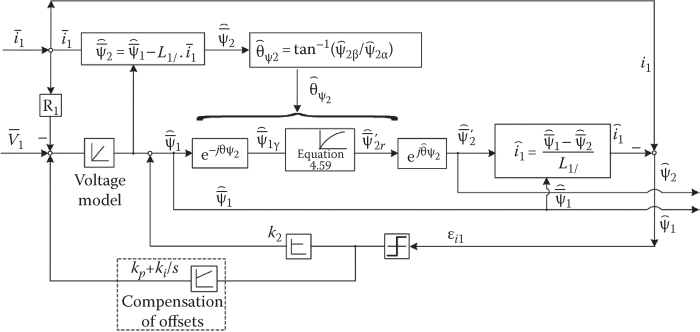
FIGURE 4.20 Observers for primary and secondary flux linkages ${\overset{⌢}{Ψ}}_{1}$ , ${\overset{⌢}{Ψ}}^{'}_{2}$ of LIMs.

Approximately, the secondary and primary resistance variations are proportional to each other as long as the LIM is loaded:

$\overset{⌢}{Δ} R_{1} = k_{R} \cdot \overset{⌢}{Δ} {R^{'}}_{2} (4.66)$

What still remains is to estimate on line the LIM speed $\overset{⌢}{U}$ :

$\overset{⌢}{U} \approx \frac{π}{τ} \cdot ({\overset{⌢}{ω}}_{{Ψ^{'}}_{2}} - (S \cdot {\overset{⌢}{ω}}_{1})); {\overset{⌢}{ω}}_{Ψ_{2}} = \frac{d {\overset{⌢}{θ}}_{Ψ_{2}}}{d t} (4.67)$

$S \cdot {\overset{⌢}{ω}}_{1} = \frac{2}{3} \cdot \frac{τ}{π} \cdot \frac{{\overset{⌢}{F}}_{x} \cdot {\overset{⌢}{R}}^{'}_{2}}{{| {\overset{⌢}{Ψ}}^{'}_{2} |}^{2}} (4.68)$

The emf compensation (voltage decoupling) is applied after the primary flux and thrust PI plus sliding mode close loops:

$\begin{matrix} V_{1 d}^{*} = (k_{p Ψ} + k_{I_{Ψ}} \cdot \frac{1}{s}) \cdot sgn (S_{Ψ_{s}}) \\ V_{1 q}^{*} = (k_{p_{F}} + k_{I_{F}} \cdot \frac{1}{s}) \cdot sgn (S_{F_{x}}) + {\overset{⌢}{ω}}_{Ψ_{1}} \cdot {\overset{⌢}{Ψ}}_{1} \\ S_{Ψ_{s}} = ε_{Ψ} + c_{Ψ} \cdot \frac{d ω_{Ψ}}{d t} \\ S_{F_{x}} = ε_{F_{x}} + c_{F_{x}} \cdot \frac{d ε_{F_{x}}}{d t} \end{matrix} (4.69)$

The block diagram of the whole control system is shown in Figure 4.21.

For a SLIM with the data in Tables 4.1 through 4.3, sample test results are shown in Figure 4.22: the stator current i_a, i_b, the primary flux, and the fast response of thrust [8].

The fast response of thrust, with sensorless control, in Figure 4.22, suggests robust state observers. At the same time, the notable thrust pulsations may be partly due to the asymmetry of stator currents (Figure 4.22), associated to static end effect caused by the small number of poles (2p = 4), via the backward primary mmf wave interaction with the secondary (as in rotary IMs with asymmetric stator currents due to the asymmetric input voltages).

Images

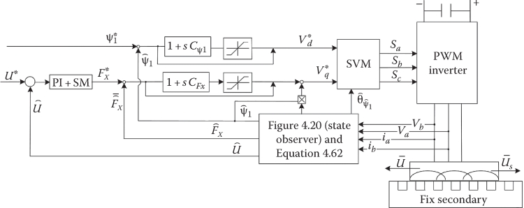
FIGURE 4.21 DTFC sensorless control of LIM.

TABLE 4.1
Motor Parameter

Images

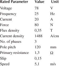
TABLE 4.2
Control Parameters

Images

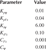
TABLE 4.3
Observer Parameters

Parameter	Value
K_p	40 + j0.10
K_I	0.005 + j0.001
K₂	–20 + j0.10

4.9 High-Speed Lim Transients and Control

An exhaustive solution for high-speed LIM transients would imply using the 3D-FE coupled field/circuit method. While such an enterprise can be profitable in special situations (though it requires prohibitive computation time), it is not for extensive studies or for the design of the control system.

For such purposes, we may start from the equivalent circuit in Figure 4.14, where L_m decreases, R′₂ increases with speed, and an additional resistance R_e is added, all these in relation to the dynamic end effect [9].

Images

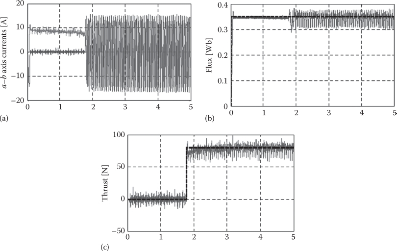
FIGURE 4.22 (a) Stator currents i_a, i_b, (b) primary flux, and (c) thrust. (After Cancelliere, P. et al., Sliding mode speed sensorless control of LIM drives, Record of LDIA-2003, Birmingham, U.K., 2003.)

$\begin{matrix} L_{m} = L_{m 0} \cdot \frac{g}{g_{0}} \cdot (1 - k_{e} (u)) \\ {R^{'}}_{2} \approx {R^{'}}_{20} = c o n s t \\ {L^{'}}_{2 l} = {L^{'}}_{2 l 0} = c o n s t \\ R_{e} \approx \frac{1 - k_{e}}{k_{e}} \cdot \frac{{R^{'}}_{2}}{s} \end{matrix} (4.70)$

These changes may be applied by including the previously mentioned variable parameters and the paralleled resistance R_e by additional equations, which have to reflect the thrust reduction due to end effect:

$\begin{matrix} {\bar{V}}_{1} = R_{1} \cdot {\bar{i}}_{1} + s \cdot {\bar{Ψ}}_{1} \\ 0 = {R^{'}}_{2} \cdot {\bar{i}}^{'}_{2} + s \cdot {\bar{Ψ}}^{'}_{2} + j \cdot \frac{τ \cdot U}{π} \cdot {\bar{Ψ}}^{'}_{2} \\ 0 = R_{e} \cdot i_{e} - s \cdot {\bar{Ψ}}_{m}; {\overset{⌢}{F}}_{x} = \frac{3}{2} \cdot \frac{π}{τ} \cdot Imag [({\bar{Ψ}}_{1} * i_{1}) - (Ψ_{m} * i_{e})] \\ {\bar{Ψ}}_{1} = L_{1 l} \cdot {\bar{i}}_{1} + L_{m} \cdot (1 - k_{e}) \cdot {\bar{i}}_{m} \end{matrix} (4.71)$

$\begin{matrix} {\bar{Ψ}}^{'}_{2} = {L^{'}}_{2 l} \cdot {i^{'}}_{2} + L_{m} \cdot (1 - k_{e}) \cdot {\bar{i}}_{m} \\ {\bar{Ψ}}_{m} = L_{m} \cdot (1 - k_{e}) \cdot {\bar{i}}_{m} \\ {\bar{i}}_{e} + {\bar{i}}_{m} = {\bar{i}}_{1} + {\bar{i}}^{'}_{2} \end{matrix}$

The last term in the thrust F_x expression relates to thrust reduction due to end effect, characteristic only to small slip frequency operation, a practical constraint met in PWM inverter supplied variable-speed LIMs.

An approximative function of speed, stator current, and slip frequency may be used to calculate k_e; as a first approximation, a linear increase of k_e with speed may be adopted in the presence of a robust DTFC or vector control system.

4.10 DTFC of High-Speed LIMs

In a simplified DTFC application, we need only a state observer to yield ${\overset{⌢}{Ψ}}_{1}$ and ${\overset{⌢}{F}}_{x}$ , in the presence of a vehicle speed sensor.

Using the voltage model in primary coordinates,

${\overset{⌢}{Ψ}}_{1} = \int ({\bar{V}}_{1}^{*} - R_{1} \cdot {\bar{i}}_{1}) d t \approx \frac{T_{e}}{1 + s T_{e}} \cdot ({\bar{V}}_{1}^{*} - R_{1} \cdot {\bar{i}}_{1}) (4.72)$

where V₁^* is the reference voltage vector; the low-pass filter deals with the offsets, but still, this simple and fast estimator is not suitable for low speeds (low-frequency ω₁, when an I–f starting strategy may be used). To calculate the thrust, ${\overset{⌢}{\bar{Ψ}}}_{m}$ and ${\overset{⌢}{\bar{i}}}_{e}$ (end effect current) have to be estimated.

From (4.72),

${\overset{⌢}{\bar{Ψ}}}_{m} = {\overset{⌢}{\bar{Ψ}}}_{1} - L_{1 l} \cdot {\bar{i}}_{1} (4.73)$

${\overset{⌢}{\bar{i}}}_{e} = \frac{{R^{'}}_{2} \cdot ({\bar{i}}_{s} - {\overset{⌢}{Ψ}}_{m} / L_{m}) - j \cdot \frac{τ}{π} \cdot U \cdot {\bar{Ψ}}_{m}}{{R^{'}}_{2} + R_{e}}; R_{e} \approx \frac{1 - k_{e}}{k_{e}} \cdot \frac{{R^{'}}_{2}}{s} (4.74)$

Also,

${\overset{⌢}{F}}_{x} = - \frac{3}{2} \cdot \frac{π}{τ} \cdot Imag [({\overset{⌢}{\bar{Ψ}}}_{1} * {\bar{i}}_{1}) - {\overset{⌢}{\bar{Ψ}}}_{m} * {\overset{⌢}{\bar{i}}}_{e}] (4.75)$

For thrust and primary-flux control, a block diagram as in Figure 4.23 [9] is thus obtained.

The end effect factor k_e, which increases with speed and depends also on Sω₁ and, for SLIMs, on Al-on-iron secondary, also on primary current, may be calculated by 1D analytical or 2(3)D FEM field theories of LIMs.

A linear variation of k_e with speed would be a first approximation.

Simulation results on an urban LIM with the data in Table 4.4 are given in Figure 4.24 [10].

Step increase of k_e in Figure 4.24d is due to the decrease in slip frequency when the thrust reference is reduced. In addition, Figure 4.24f reflects the necessity to consider R_e, as the estimated thrust is smaller than the actual thrust. Other pertinent LIM control systems are introduced in Refs. [10–14]].

Images

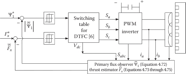
FIGURE 4.23 DTFC of high-speed LIM.

TABLE 4.4
Urban LIM Data

Images

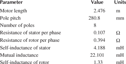
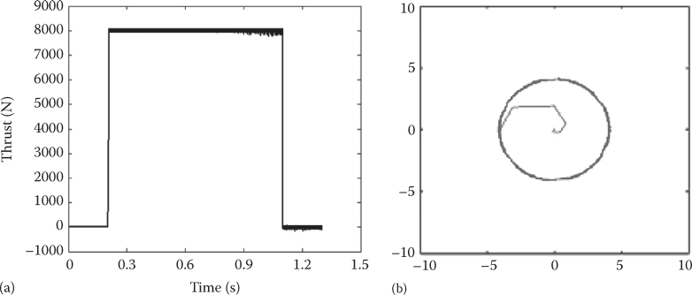
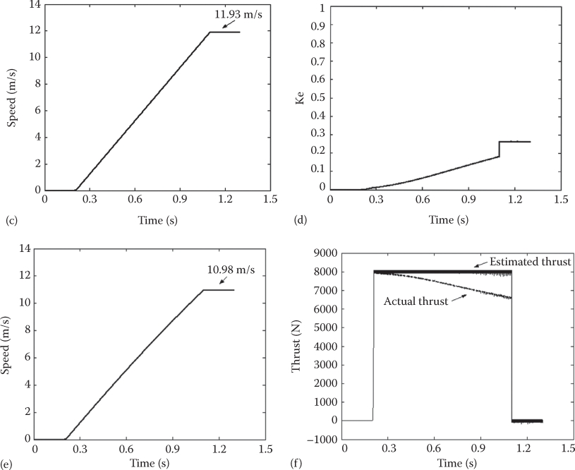
FIGURE 4.24 Urban SLIM thrust control response: (a) thrust response and (b) primary-flux response. Urban SLIM thrust control response: (c) speed response, (d) end effect factor k_e, (e) actual speed response with end effect, and (f) estimated thrust and actual thrust with R_e neglected. (After Wang, K. et al., Direct thrust control of LIM considering end effects, Record of LDIA-2007, 2007; Takahashi, I. and Ide, Y., IEEE Trans., IA-29(1), 161, 1993.)

4.11 Summary

Circuit models for LIMs needed to investigate transients and control and design stem from the equivalent circuit of rotary IM, with adequate modifications.
To simplify the control of low-speed (or short travel) LIMs, they are kept in the negligible dynamic end effect conditions.
The divide between low or high speed (low or notable dynamic end effect) is settled in this chapter by the condition that the exit end effect wave depth of penetration within LIM primary from the entry end is less than 10% of primary length. It turns out that this condition depends only on the number of poles 2p, equivalent goodness factor G_e, and slip S. The equivalent goodness factor included edge effect, skin effect, slot opening, airgap fringing, and magnetic saturation (for SLIMs with Al-on-iron secondary)
The low-speed LIM equivalent circuit parameters are then calculated for
- Flat DLIM
- Flat SLIM with Al-on-iron secondary
- Flat SLIM with ladder secondary
- Tubular SLIM with cage secondary

The parameters of the equivalent circuit, mainly L_m, R′₂, L^′₂_l (for Al-on-iron secondary), depend on slip frequency Sω₁, airgap variation (Lm), and on the stator mmf (current)—due to magnetic saturation.

Equivalent (fictitious) double cage (ladder) may represent such variations based on frequency response tests applied to curve fitting of field theory results:

For constant stator current, a maximum thrust/current slip frequency is obtained (Sω₁)_k; this is notably lower than the one for which the net normal force (in SLIM) passes through zero (an idea used for some LIM-propulsed urban MAGLEVs); consequently, lower efficiency is expected for zero net normal force.
In flat SLIMs with Al-on-iron secondary, the contribution of the solid back iron of secondary (even if divided transversally into three slabs (“laminations”)) to total thrust and to the equivalent airgap is notable. Running such LIMs at constant slip frequency Sω₁ would render the parameters variable only with stator current (due to magnetic saturation) and thus easier to use in assessing thoroughly the steady-state performance of LIM.
To limit the influence of transverse edge effect on secondary resistance, the overhangs of aluminum (or end slabs in ladder secondaries) should not be shorter than τ/π (c – a ≈ τ/π).
The flat SLIM with ladder secondary, for short travel (when its cost is acceptable), is shown capable, with good performance and thrust density (η ≥ 0.8, cos ϕ > 0.65) (B_g₁ ≈ 0.6–0.7 T) for airgaps of 1.0–2.0 mm at maximum speeds below 10 m/s.
As the normal force in SLIM is unilateral, and large for ladder secondary, it may be used for mover (vehicle) suspension (partial or total).
The tubular LIM with cage secondary, adequate for very short travel (less than 1.5–2 m in general) and airgap of 1–1.5 mm, is credited with even better thrust density, efficiency, and power factor, due to the absence of radial force and stator end coils and edge effect, despite lower speeds (less than 6 m/s maximum speed).
Circuit models for high speed introduce a reduction by (1 – k_e) of emf and then a new end effect impedance Z_e in parallel with jω₁L_m: Z_e = ((1 – k_e)/k_e)Z′₂_c is added.

Z′₂_c is the conventional airgap plus secondary part of the equivalent circuit, typical to low-speed LIMs:

The end effect factor k_e increases with speed, for a given high-speed LIM geometry, but it also increases when slip frequency decreases; a linear increase of k_e with speed is acceptable at given slip S.
The equivalent circuits with end effects have been verified in experiments enquiring thrust reduction and then efficiency and power factor reduction and finally for secondary Joule losses [14].
Identifying the equivalent circuit parameters with dynamic end effect, for a given LIM, may also be done by processing key running tests (at key speed and loads) by regressive methods of curve fitting.
Also, simplified analytical expressions for k_e(U), derived from 1D field theories, are given and checked against two representative SLIMs.
The separate treatment of transients for low- and high-speed LIMs (low or notable dynamic end effect) by space vector models is then approached.
The similarity of low dynamic end effect (low-speed) LIM space vector models with those of rotary IMs is striking: thrust instead of torque, linear speed versus angular speed, and no number of pole pairs p but τ (pole pitch) present in the thrust expression.
Motoring and generating vector (space–phasor) diagrams are presented to illustrate that, in both operation modes, the amplitude of stator flux vector ${\bar{Ψ}}_{1}$ is greater than that of secondary flux ${\bar{Ψ}}^{'}_{2} | : (| {\bar{Ψ}}_{1} | > | {\bar{Ψ}}^{'}_{2} |) |$ .
The equations of low-speed LIMs in space phasor for constant speed may be solved analytically and reveal two complex eigen values γ_1,2; the real parts of γ_1,2 are negative at less than critical slip frequencies (Sω₁ < (Sω₁)_k); (Sω₁)_k corresponds to maximum thrust.
As the flux initiation in LIMs is not very fast, it is good to have it first “installed” even if as a single voltage vector (say ${\bar{Ψ}}_{1}$ aligned to phase a axis), before activating the speed control.
Three control techniques, one scalar (I–Sf₁ close-loop control), two vectorial (one secondary-flux orientation control-FOC), and one direct thrust and primary-flux control DTFC.
The simplicity and robustness of I–Sf₁ scalar control are notable, if PI plus sliding mode speed control is provided, but fast thrust transient response is not guaranteed.
FOC of LIMs reveals the linear thrust/speed, F_x(U), curves, typical for rotor flux orientation control in rotary IMs.
A combined indirect vector current and voltage control FOC is described, to secure fast thrust response and increased stability and dynamic robustness, especially if a position sensor (with speed calculation) is available for positioning applications.
To illustrate DTFC of low-speed LIMs, a motion-sensorless speed control system with space vector modulation and PI + SM primary- and secondary-flux observer and thrust and speed estimators has been introduced; corrections for secondary (and primary) resistances are introduced together with magnetization inductance L_m and L_m(Im) curve online adjustment. L_m varies not only due to magnetic saturation but also due to airgap inevitable fluctuation; this justifies its online correction. The response in thrust and flux step variation are remarkably fast and stable in experiments.
For high-speed (large end effect) LIMs’ transients and control, simplified corrections of L_m (it becomes (1 – k_e) · L_m) and addition of a parallel resistive circuit R_e = ((1 – k_e)/k_e)R′₂/s are introduced in the space–phasor model equations to model dynamic end effects. The dynamic end effect factor k_e (which decreases the emf and the thrust and causes additional secondary Joule losses) has to be calculated (or calibrated upon commissioning the LIM drive), but it may also be considered to increase linearly with speed increase and with slip decrease; an inferior limit for |S·f₁| might keep k_e just linearly varying with speed for a given LIM.
An implementation of a DTFC of an existing urban LIM shows notable end effect (k_e goes up to 0.3) with a step increase for a step thrust reference reduction. Again, it is G_e, 2p and S that influence k_e (end effect influence, with speed implicit by frequency f₁ (in G_e) and slip, with the given pole pitch of primary winding).
Short (mover) secondary and long (fix) primary LIMs have not been investigated in this chapter, even in the form of wound secondary on board of mover with energy “induction” on the vehicle, without power collection; it will be treated shortly only in the chapter on MAGLEV, as they did not reach markets yet and are heavily in competition with PMs or dc excited long primary stator linear synchronous motors.
Proposed decades ago for oscillators, short secondary long primary LIMs have been since outperformed by PM linear synchronous resonant single-phase oscillators; this is the reason why they have not been treated here in any detail (see [3] for a field theory of short secondary long primary LIMs).
Now that we have elucidated field theories, circuit models, the transients and control of LIMs, the design of LIMs will be approached separately for low-speed (low end effect) LIMs and for high-speed (notable end effect) LIMs.

References

1. I. Boldea and S.A. Nasar, Linear Motion Electromagnetic Devices, Taylor & Francis, New York, 2001.

2. A. Krawczyk and J. Tegopoulous, Numerical Modelling of Eddy Currents, Oxford University Press, New York, 1993.

3. I. Boldea and S.A. Nasar, Linear Motion Electromagnetic Systems, John Wiley, New York, 1985 (Chapter 4).

4. J.F. Gieras, G.E. Dawson, and A.R. Eastham, A new longitudinal end factor for LIMs, IEEE Trans., EC-2(1), 1987, 152–159.

5. C.M.A.R. Cabral, Analysis of LIMs using new longitudinal end effect factors, Record of LDIA-2003, Birmingham, U.K., pp. 291–294.

6. I. Boldea and S.A. Nasar, Electric Drives, 2nd edn., CRC Press, Taylor & Francis, New York, 2006.

7. G. Bucci, S. Meo, A. Ometo, and S. Scarano, The control of LIM by a generalization of standard vector techniques, IEEE—IAS Annual Meeting Conference, Bologna, Italy, 1995.

8. P. Cancelliere, V. Delli Colli, F. Marignetti, and I. Boldea, Sliding mode speed sensorless control of LIM drives, Record of LDIA-2003, Birmingham, U.K.

9. K. Wang, L. Shi, and Y. Li, Direct thrust control of LIM considering end effects, Record of LDIA-2007.

10. I. Takahashi and Y. Ide, Decoupling thrust and attractive forces of LIM using space vector control inverter, IEEE Trans., IA-29(1), 1993, 161–167.

11. B.-I. Kwon, K.-I. Woo, and S. Kim, Finite element analysis of direct thrust—Controlled LIM, IEEE Trans., MAG-35(3), 1999, 1306–1309.

12. M. Abbasian, Adaptive input—Output control of linear induction motor considering the end effect, Record of ICEM, 2010, Rome, Italy.

13. A. Gastli, Improved field oriented control of a LIM having joints in its secondary conductors, IEEE Trans., EC-17(3), 2002, 349–355.

14. W. Xu, J. G. Zhu, Y. Zhang, Z. Li, Y. Wung, Y. Guo, and Y. Li, Equivalent circuits for single—Sided linear induction motors, IEEE Trans., IA-46(6), 2010, 2410–2423.

..................Content has been hidden....................

You can't read the all page of ebook, please click here login for view all page.

Table of Contents for Chapter 4 Linear Induction Motors: Circuit Theories, Transients, and Control

Create new playlist

Sign In

Sign Up

Circuit Theories, Transients, and Control

Table of Contents for
Chapter 4 Linear Induction Motors: Circuit Theories, Transients, and Control