Chapter 9
Distribution System Voltage Regulation
Nothing is so firmly believed as what we least know.
M.E. De Montaigne, Essays, 1580
Talk sense to a fool and he calls you foolish.
Euripides, The Bacchae, 407 B. C.
But talk nonsense to a fool and he calls you a genius.
Turan Gönen
9.1 Basic Definitions
Voltage regulation: The percent voltage drop of a line (e.g., a feeder) with respect to the receiving-end voltage. Therefore,
% regulation=|Vs|−|Vr||Vr|×100(9.1)
Voltage drop: The difference between the sending-end and the receiving-end voltages of a line
Nominal voltage: The nominal value assigned to a line or apparatus or a system of a given voltage class
Rated voltage: The voltage at which performance and operating characteristics of apparatus are referred
Service voltage: The voltage measured at the ends of the service-entrance apparatus
Utilization voltage: The voltage measured at the ends of an apparatus
Base voltage: The reference voltage, usually 120 V
Maximum voltage: The largest 5-min average voltage
Minimum voltage : The smallest 5-min voltage
Voltage spread: The difference between the maximum and minimum voltages, without voltage dips due to motor starting
9.2 Quality of Service and Voltage Standards
In general, performance of distribution systems and quality of the service provided are measured in terms of freedom from interruptions and maintenance of satisfactory voltage levels at the customer’s premises that are within limits appropriate for this type of service. Due to economic considerations, an electric utility company cannot provide each customer with a constant voltage matching exactly the nameplate voltage on the customer’s utilization apparatus.
Therefore, a common practice among the utilities is to stay with preferred voltage levels and ranges of variation for satisfactory operation of apparatus as set forth by the American National Standards Institute (ANSI) Standard [2]. In many states, the ANSI standard is the basis for the state regulatory commission rulings on setting forth voltage requirements and limits for various classes of electric service.
In general, based on experience, too-high steady-state voltage causes reduced light bulb life, reduced life of electronic devices, and premature failure of some types of apparatus. On the other hand, too-low steady-state voltage causes lowered illumination levels, shrinking of TV pictures, slow heating of heating devices, difficulties in motor starting, and overheating and/or burning out of motors. However, most equipment and appliances operate satisfactorily over some range of voltage so that a reasonable tolerance is allowable.
The nominal voltage standards for a majority of the electric utilities in the United States to serve residential and commercial customers are
- 120/240 V three-wire single phase
- 240/120 V four-wire three-phase delta
- 208Y/120 V four-wire three-phase wye
- 480Y/277 V four-wire three-phase wye
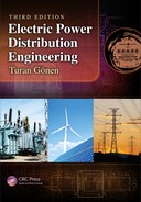
As shown in Figure 9.1, the voltage on a distribution circuit varies from a maximum value at the customer nearest to the source (first customer) to a minimum value at the end of the circuit (last customer). For the purpose of illustration, Table 9.1 gives typical secondary voltage standards applicable to residential and commercial customers. These voltage limits may be set by the state regulatory commission as a guide to be followed by the utility.
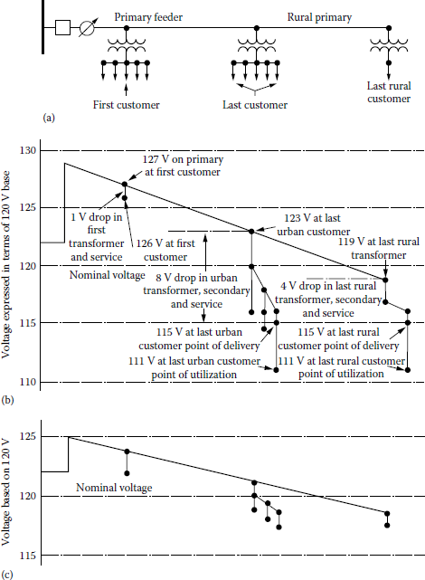
Illustration of voltage spread on a radial primary feeder: (a) one-line diagram of a feeder circuit, (b) voltage profile at peak-load conditions, and (c) voltage profile at light-load conditions.
Typical Secondary Voltage Standards Applicable to Residential and Commercial Customers
Voltage Limits |
|||
|---|---|---|---|
At Point of Delivery |
At Point of Utilization |
||
Nominai Voltage Class |
Maximum |
Minimum |
Minimum |
120/240 V 1ϕ and 240/120 V 3ϕ |
|||
Favorable zone, range A |
126/252 |
114/228 |
110/220 |
Tolerable zone, range B |
127/254 |
110/220 |
106/212 |
Extreme zone, emergency |
130/260 |
108/216 |
104/208 |
208Y/120 V 3ϕ |
|||
Favorable zone, range A |
218Y/126 |
197Y/114 |
191Y/110 |
Tolerable zone, range B |
220Y/127 |
191Y/110 |
184Y/106 |
Extreme zone, emergency |
225Y/130 |
187Y/108 |
180Y/104 |
408Y/277 V 3ϕ |
|||
Favorable zone, range A |
504Y/291 |
456Y/263 |
440Y/254 |
Tolerable zone, range B |
508Y/293 |
440Y/254 |
424Y/245 |
Extreme zone, emergency |
520Y/300 |
432Y/249 |
416Y/240 |
As can be observed in Table 9.1, for any given nominal voltage level, the actual operating values can vary over a large range. This range has been segmented into three zones, namely, (1) the favorable zone or preferred zone, (2) the tolerable zone, and (3) the extreme zone. The favorable zone includes the majority of the existing operating voltages and the voltages within this zone (i.e., range A) to produce satisfactory operation of the customer’s equipment.
The distribution engineer tries to keep the voltage of every customer on a given distribution circuit within the favorable zone. Figure 9.1 illustrates the results of such efforts on urban and rural circuits. The tolerable zone contains a band of operating voltages slightly above and below the favorable zone. The operating voltages in the tolerable zone (i.e., range B) are usually acceptable for most purposes. For example, in this zone, the customer’s apparatus may be expected to operate satisfactorily, although its performance may perhaps be less than warranted by the manufacturer.
However, if the voltage in the tolerable zone results in unsatisfactory service of the customer’s apparatus, the voltage should be improved. The extreme or emergency zone includes voltages on the fringes of the tolerable zone, usually within 2% or 3% above or below the tolerable zone. They may or may not be acceptable depending on the type of application. At times, the voltage that usually stays within the tolerable zone may infrequently exceed the limits because of some extraordinary conditions. For example, failure of the principal supply line, which necessitates the use of alternative routes or voltage regulators being out of service, can cause the voltages to reach the emergency limits.
However, if the operating voltage is held within the extreme zone under these conditions, the customer’s apparatus may still be expected to provide dependable operation, even though not the standard performance. However, voltages outside the extreme zone should not be tolerated under any conditions and should be improved right away. Usually, the maximum voltage drop in the customer’s wiring between the point of delivery and the point of utilization is accepted as 4 V based on 120 V.
9.3 Voltage Control
To keep distribution-circuit voltages within permissible limits, means must be provided to control the voltage, that is, to increase the circuit voltage when it is too low and to reduce it when it is too high. There are numerous ways to improve the distribution system’s overall voltage regulation. The complete list is given by Lokay [1] as
- Use of generator voltage regulators
- Application of voltage-regulating equipment in the distribution substations
- Application of capacitors in the distribution substation
- Balancing of the loads on the primary feeders
- Increasing of feeder conductor size
- Changing of feeder sections from single phase to multiphase
- Transferring of loads to new feeders
- Installing of new substations and primary feeders
- Increasing of primary voltage level
- Application of voltage regulators out on the primary feeders
- Application of shunt capacitors on the primary feeders
- Application of series capacitors on the primary feeders
The selection of a technique or techniques depends upon the particular system requirement. However, automatic voltage regulation is always provided by (1) bus regulation at the substation, (2) individual feeder regulation in the substation, and (3) supplementary regulation along the main by regulators mounted on poles. Distribution substations are equipped with load-tap-changing (LTC) transformers that operate automatically under load or with separate voltage regulators that provide bus regulation.
Voltage-regulating apparatus are designed to maintain automatically a predetermined level of voltage that would otherwise vary with the load. As the load increases, the regulating apparatus boosts the voltage at the substation to compensate for the increased voltage drop in the distribution feeder. In cases where customers are located at long distances from the substation or where voltage drop along the primary circuit is excessive, additional regulators or capacitors, located at selected points on the feeder, provide supplementary regulation. Many utilities have experienced that the most economical way of regulating the voltage within the required limits is to apply both step voltage regulators and shunt capacitors.
Capacitors are installed out on the feeders and on the substation bus in adequate quantities to accomplish the economic power factor. Many of these installations have sophisticated controls designed to perform automatic switching. A fixed capacitor is not a voltage regulator and cannot be directly compared to regulators, but, in some cases, automatically switched capacitors can replace conventional step-type voltage regulators for voltage control on distribution feeders.
9.4 Feeder Voltage Regulators
Feeder voltage regulators are used extensively to regulate the voltage of each feeder separately to maintain a reasonable constant voltage at the point of utilization. They are either the induction type or the step type. However, since today’s modern step-type voltage regulators have practically replaced induction-type regulators, only step-type voltage regulators will be discussed in this chapter.
Step-type voltage regulators can be either (1) station type, which can be single or three phase and which can be used in substations for bus voltage regulation (BVR) or individual feeder voltage regulation; or (2) distribution type, which can be only single phase and used pole-mounted out on overhead primary feeders. Single-phase step-type voltage regulators are available in sizes from 25 to 833 kVA, whereas three-phase step-type voltage regulators are available in sizes from 500 to 2000 kVA.
For some units, the standard capacity ratings can be increased by 25%–33% by forced-air cooling. Standard voltage ratings are available from 2,400 to 19,920 V, allowing regulators to be used on distribution circuits from 2,400 to 34,500 V grounded-wye/19,920 V multigrounded-wye. Stationtype step voltage regulators for BVR can be up to 69 kV.
A step-type voltage regulator is fundamentally an autotransformer with many taps (or steps) in the series winding. Most regulators are designed to correct the line voltage from 10% boost to 10% buck (i.e., ±10%) in 32 steps, with a ⅝ % voltage change per step.
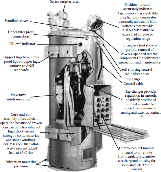
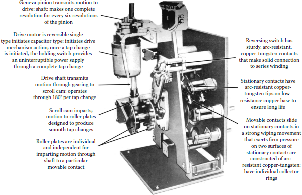
(Note that the full voltage regulation range is 20%, and therefore if the 20% regulation range is divided by the 32 steps, a percent regulation per step is found.) If two internal coils of a regulator are connected in series, the regulator can be used for ±10% regulation; when they are connected in parallel, the current rating of the regulator would increase to 160%, but the regulation range would decrease to ±5%. Figure 9.2 shows a typical single-phase 32-step pole-type voltage regulator; Figure 9.3 shows its application on a feeder with essential components. Figure 9.4 shows typical platform-mounted voltage regulators. Individual feeder regulation for a large utility can be provided at the substation by a bank of distribution voltage regulators, as shown in Figure 9.5.
Typical single-phase 32-step pole-type voltage regulator used for 167 kVA or below.
(McGraw-Edison Company, Belleville, NJ.)
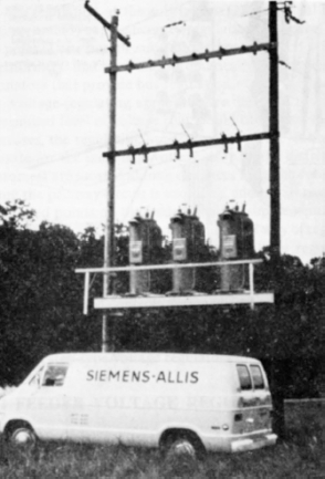
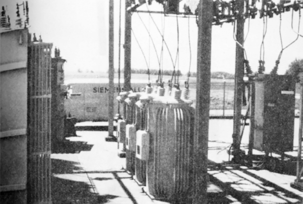
Individual feeder voltage regulation provided by a bank of distribution voltage regulators.
(Siemens-Allis Company.)
In addition to its autotransformer component, a step-type regulator also has two other major components, namely, the tap-changing mechanism and the control mechanism, as shown in Figure 9.2. Each voltage regulator ordinarily is equipped with the necessary controls and accessories so that the taps are changed automatically under load by a tap changer that responds to a voltage-sensing control to maintain a predetermined output voltage. By receiving its inputs from potential transformer (PT) and current transformer (CT), the control mechanism provides control of voltage level and bandwidth (BW).
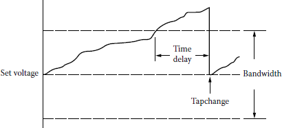
One of such control mechanisms is a voltage regulating relay (VRR), which controls tap changes. As illustrated in Figure 9.6, this relay has the following three basic settings that control tap changes:
- Set voltage: It is the desired output of the regulator. It is also called the set point or band center.
- Bandwidth: Voltage regulator controls monitor the difference between the measured voltage and the set voltage. Only when the difference exceeds one half of the BW will a tap change start.
- Time delay (TD): It is the waiting time between the time when the voltage goes out of the band and when the controller initiates the tap change. Longer TDs reduce the number of tap changes. Typical TDs are 10–120 s.
Furthermore, the control mechanism also provides the ability to adjust line-drop compensation by selecting the resistance and reactance settings, as shown in Figure 9.7. Figure 9.8 shows a standard direct-drive tap changer. Figure 9.9 shows four-step auto-booster regulators. Auto-boosters basically are single-phase regulating autotransformers, which provide four-step feeder voltage regulation without the high degree of sophistication found in 32-step regulators. They can be used on circuits rated 2.4 to 12 kV delta and 2.4/4.16 to 19.92/34.5 kV multigrounded-wye. The auto-booster unit can have a continuous current rating of either 50 or 100 A. Each step represents either 1½% or 2½% voltage change depending on whether the unit has a 6% or 10% regulation range, respectively. They cost much less than the standard voltage regulators.
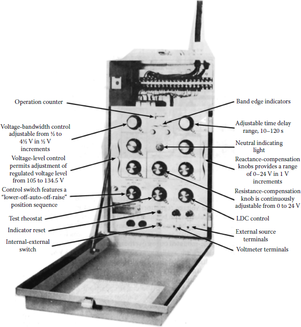
Features of the control mechanism of a single-phase 32-step voltage regulator.
(McGraw-Edison Company, Belleville, NJ.)
Standard direct-drive tap changer used through 150 kV BIL, above 219 A.
(McGraw-Edison Company, Belleville, NJ.)
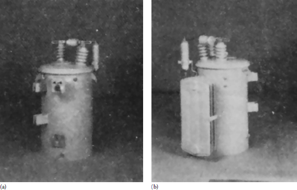
Four-step auto-booster regulators: (a) 50 A unit and (b) 100 A unit.
(McGraw-Edison Company, Belleville, NJ.)
9.5 Line-Drop Compensation
Voltage regulators located in the substation or on a feeder are used to keep the voltage Constant at a fictitious regulation or regulating point (RP) without regard to the magnitude or power factor of the load. The regulation point is usually selected to be somewhere between the regulator and the end of the feeder. This automatic voltage maintenance is achieved by dial settings of the adjustable resistance and reactance elements of a unit called the line-drop compensator (LDC) located on the control panel of the voltage regulator. Figure 9.10 shows a simple schematic diagram and phasor diagram of the control circuit and LDC circuit of a step or induction voltage regulator. Determination of the appropriate dial settings depends upon whether or not any load is tapped off the feeder between the regulator and the regulation point.
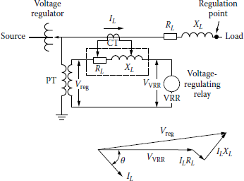
Simple schematic diagram and phasor diagram of the control circuit and line-drop compensator circuit of a step or induction voltage regulator.
(From Westinghouse Electric Corporation, Electric Utility Engineering Reference Book-Distribution Systems, Vol. 3, Westinghouse Electric Corporation, East Pittsburgh, PA, 1965.)
If no load is tapped off the feeder between the regulator and the regulation point, the R dial setting of the LDC can be determined from
Rset=CTpPTN×Reff Ω(9.2)
where
CTP is the rating of the current transformer’s primary
PTN is the potential transformer’s turns ratio = Vpri/Vsec
Reff is the effective resistance of a feeder conductor from regulator station to regulation point, Ω
Reff=ra×ℓ−s12 Ω(9.3)
where
ra is the resistance of a feeder conductor from regulator station to regulation point, Ω/mi per conductor
s1 is the length of three-phase feeder between regulator station and substation, mi (multiply length by 2 if feeder is in single phase)
ℓ is the primary feeder length, mi
Also, the X dial setting of the LDC can be determined from
Xset=CTpPTN×Xeff Ω(9.4)
where Xeff is the effective reactance of a feeder conductor from regulator to regulation point, Ω
Xeff=xL×ℓ−s12 Ω(9.5)
and
xL=xa+xd Ω/mi(9.6)
where
xa is the inductive reactance of individual phase conductor of feeder at 12-in spacing, Ω/mi
xd is the inductive-reactance spacing factor, Ω/mi
xL is the inductive reactance of feeder conductor, Ω/mi
Note that since the R and X settings are determined for the total connected load, rather than for a small group of customers, the resistance and reactance values of the transformers are not included in the effective resistance and reactance calculations.
If load is tapped off the feeder between the regulator station and the regulation point, the R dial setting of the LDC can still be determined from Equation 9.2, but the determination of the Reff is somewhat more involved. Lokay [1] gives the following equations to calculate the effective resistance:
Reff=∑ni=1|VDR|i|IL| Ω(9.7)
and
n∑i−1|VDR|i=|IL,1|× ra,1×l1+|IL,2|× ra,2×l2+⋅⋅⋅+|IL,n|× ra,n×ln(9.8)
where
||VDR||i is the voltage drop due to line resistance of ith section of feeder between regulator station and regulation point, V/section
∑ni=1|VDR|i is the total voltage drop due to line resistance of feeder between regulator station and regulation point, V
||IL|| is the magnitude of load current at regulator location, A
||IL,i|| is the magnitude of load current in ith feeder section, A
ra,i is the resistance of a feeder conductor in ith section of feeder, Ω/mi
ℓi is the length of ith feeder section, mi
Also, the X dial setting of the LDC can still be determined from Equation 9.4, but the determination of the Xeff is again somewhat more involved. Lokay [1] gives the following equations to calculate the effective reactance:
Xeff=∑ni=1|VDX|i|IL| Ω(9.9)
and
n∑i=1|VDX|i=|IL,1|×XL,1×I1+|IL,2|×XL,2×I2+⋅⋅⋅+|IL,n|×XL,n×In(9.10)
where
||VDX||i is the voltage drop due to line reactance of ith section of feeder between regulator station and regulation point, V/section
∑ni=1|VDX|i is the total voltage drop due to line reactance of feeder between regulator station and regulation point, V
XL,1 is the inductive reactance [as defined in Equation 9.6] of ith section of feeder, Ω/mi
Since the methods just described to determine the effective R and X are rather involved, Lokay [1] suggests as an alternative and practical method to measure the current (IL) and voltage at the regulator location and the voltage at the RP. The difference between the two voltage values is the total voltage drop between the regulator and the regulation point, which can also be defined as
VD=|IL|× Reff×cosθ+|IL|×Xeff×sinθ(9.11)
from which the Reff and Xeff values can be determined easily if the load power factor of the feeder and the average R/X ratio of the feeder conductors between the regulator and the RP are known.
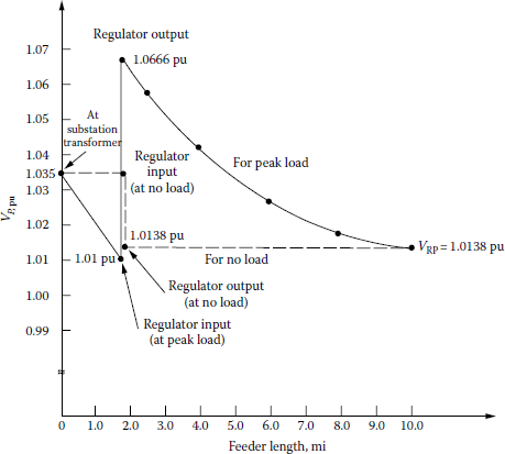
Figure 9.11 gives an example for determining the voltage profiles for the peak and light loads. Note that the primary-feeder voltage values are based on a 120 V base.
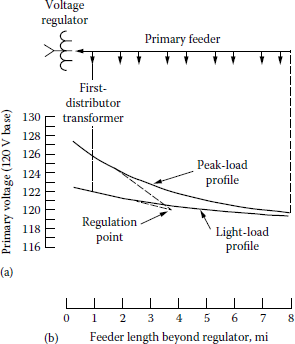
It represents one-line diagram and voltage profiles of a feeder with distributed load beyond a voltage regulator location: (a) one-line diagram and (b) peak- and light-load profiles showing fictitious RP for LDC settings. It is assumed that the conductor size between regulator and first distribution transformer is #2/0 copper conductor with 44-in flat spacing with resistance and reactance of 0.481 and 0.718 2/mi, respectively. The PT and CT ratios of the voltage regulator are 7960: 120 and 200: 5, respectively. Distance to fictitious RP is 3.9 mi. LDC settings are
Rset=200×1207960×0.481×3.9=5.656
Xset=200×1207960×0.718×3.9=8.4428
Voltage-regulating relay setting is 120.1 V. (From [1].)
Example 9.1
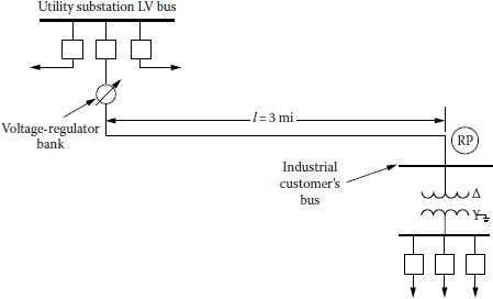
This example investigates the use of step-type voltage regulation (control) to improve the voltage profile of distribution systems. Figure 9.12 illustrates the elements of a distribution substation that is supplied from a subtransmission loop and feeds several radial primary feeders.
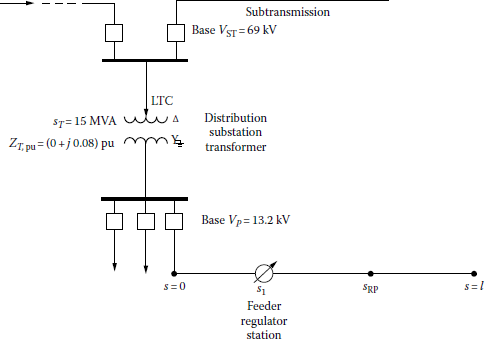
The substation LTC transformer can be used to regulate the primary distribution voltage (VP) bus, holding VP constant as both the subtransmission voltage (VST) and the IZT voltage drop in the substation transformer vary with load. If the typical primary-feeder main is voltage-drop-limited, it can be extended further and/or loaded more heavily if a feeder voltage regulator bank is used wisely. In Figure 9.12, the feeder voltage regulator, indicated with the symbol shaped as a 0 with an arrow going through it, is located at the point s = s1, and it varies its boost and buck automatically to hold a set voltage at the RP, that is, at s = sRP.
Typical LTC and feeder regulator data: The abbreviation VRR stands for voltage-regulating relay (or solid-state equivalent thereof), and it is adjustable within the approximate range from 110 to 125 V. The VRR measures the voltage at the RP, that is, VRP, by means of the LDC.
The LDC has R and X settings, which are both adjustable within the approximate range from 0 to 24 Ω (often called volts because the CTs used with regulators have 1.A secondaries).
The BW of the VRR is adjustable within the approximate range from ±¾ to ±1½ V based on 120 V. The TD is adjustable between about 10 and 120 s.
The location of the RP is controlled by the R and X settings of the LDC. If the R and X settings are set to be zero, the regulator regulates the voltage at its local terminal to the setting of the VRR ± BW. In this example, sRP = s1.
Overloading of step-type feeder regulators ANSI standards provide for regulator overload capacity as listed in Table 9.2 in case the full 10% range of regulation is not required. All modern regulators are provided with adjustments to reduce the range to which the motor can drive the tap-changer switching mechanism.
Overloading of Step-Type Feeder Regulators
Reduced Range of Regulation (%) |
Percent of Normal Load Current |
|---|---|
±10.00 |
100 |
±8.75 |
110 |
±7.50 |
120 |
±6.25 |
135 |
±5.00 |
160 |
Good advantage sometimes can be taken of this designed overload type of limited-range operation. However, if load growth occurs, both a larger range of regulation and a larger regulator size (kilovoltamperes or current) can be expected to be needed. Table 9.3 gives some typical single-phase regulator sizes.
Some Typical Single-Phase Regulator Sizes
Single Phase kVA |
Volts |
Amps |
CTPa |
PTNb |
|---|---|---|---|---|
25 |
2500 |
100 |
100 |
20 |
⋮ |
⋮ |
⋮ |
⋮ |
⋮ |
125 |
2500 |
500 |
500 |
20 |
38.1 |
7620 |
50 |
50 |
63.5 |
57.2 |
7620 |
75 |
75 |
63.5 |
76.2 |
7620 |
100 |
100 |
63.5 |
114.3 |
7620 |
150 |
150 |
63.5 |
167 |
7620 |
219 |
250 |
63.5 |
250 |
7620 |
328 |
400 |
63.5 |
a Ratio of the current transformer contained within the regulator. (Here, the ratio is the high-voltage-side ampere rating because the low-voltage rating is 1.0 A.)
b Ratio of the potential transformer contained within the regulator. (All potential transformer secondaries are 120 V.)
Substation data Make the following assumptions:
- Base MVA3ϕ = 15 MVA
- Subtransmission base VL–L = 69 kV
- Primary base VL–L = 13.2 kV
The substation transformer is rated 15 MVA, 69–7.62/13.2 kV grounded-wye and has a per unit impedance (ZT,pu) of 0 + j0.08 based on its ratings. Its three-phase LTC can regulate ±10% voltage in 32 steps of 5/8% each.
Load flow data: Assume that the maximum subtransmission voltage (max VST) is 72.45 kV or 1.05 pu, which occurs during the off-peak period at which the off-peak kilovoltamperage is 0.25 pu with a leading power factor of 0.95. The minimum subtransmission voltage (min VST) is 69 kV or 1.00 pu, which occurs during the peak period at which the peak kilovoltamperage is 1.00 pu with a lagging power factor of 0.85.
Voltage data and voltage criteria: Assume that the maximum secondary voltage is 125 V or 1.0417 pu V (based on 120 V) and the minimum secondary voltage is 116 V or 0.9667 pu V, and that the maximum voltage drop in secondaries is 0.035 pu V.
Assume that the maximum primary voltage (max VP) is 1.0417 pu V at zero load, and that at annual peak load, the maximum primary voltage is 1.0767 pu V (1.0417 + 0.035) considering the nearest secondary to the regulator and the minimum primary voltage is 1.0017 pu V (0.9667 + 0.035) considering the most remote secondary.
Feeder data: Assume that the annual peak load is 4000 kVA, at a lagging power factor of 0.85, and is distributed uniformly along the 10-mi-long feeder main. The main has 266.8 kcmil all-aluminum conductors (AACs) with 37 strands and 53-in geometric mean spacing. Use 3.88 × 10⁻⁶ pu VD/ (kVA · mi) at 0.85 lagging power factor as the constant K.
Assume that the substation transformer LTC is used for BVR. Use a BW of ±1.0 V or (1 V/120 V) = 0.0083 pu V. Also use rounded figures of 1.075 and 1.000 pu V for the maximum and minimum primary voltages at peak load, respectively.
- Specify the setting of the VRR for the highest allowable primary voltage (VP), BW being considered, then round the setting to a convenient number.
- Find the maximum number of steps of buck and boost that will be required.
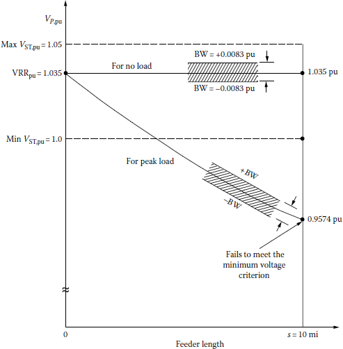
- Sketch voltage profiles of the feeder being considered for zero load and for the annual peak load. Label the significant voltage values on the curves.
Solution
- Since the LDC of the regulator is not used,
Rset=0 and Xset=0
Therefore, the setting of the VRR for the highest allowable primary voltage, BW being considered, occurs at the zero load and is
VPR=(Vp)max−BW=1.0417−0.0083=1.0334 pu V≅1.035 pu V=124.2 V
- To find the maximum number of buck and boost that will be required, the highest allowable primary voltages at off-peak and on-peak have to be found. Therefore, at off-peak,
−Vp, pu=−VST,pu−−Ip, pu×−ZT, pu(9.12)
where
VST,pu is the per unit subtransmission voltage at primary side of the substation transformer = 1.05/∠0° pu V
IP,pu is the per unit no-load primary current at substation (transformer) = 0.2381 pu A = per unit impedance of substation transformer
ZT,pu = 0 + j0.08 pu Ω
Therefore,
VP,pu=1.05−(0.2381)(cos θ+j sin θ)(0+j0.08)=1.05−(0.2381)(0.95+j0.3118)(0+j0.08)=1.0589 pu V
whereas at on-peak,
VP, pu=1.0 - (1.00)(0.85 - j0.53)(0 + j0.08)=0.9602 pu V
Since the LTC of the substation can regulate ±10% voltage in 32 steps of 5/8% volts (or 0.00625 pu V) each, the maximum number of steps of buck required, at off-peak, is
No. of steps=VP, pu−VRRpu0.00625=1.0589−1.0350.00625≅3 or 4 steps(9.13)
and the maximum number of steps of boost required, at peak, is
No. of steps=VP, pu−VRRpu0.00625=1.035−0.96020.00625≅12 steps(9.14)
- To sketch voltage profiles of the primary feeder for the annual peak load, the total voltage drop of the feeder has to be known. Therefore,
∑VDpu=K×S×ℓ2=(3.88×10⁻⁶)(4000 kVA)(10mi2)=0.0776 pu V(9.15)
and thus the minimum primary-feeder voltage at the end of the 10 mi feeder, as shown in Figure 9.13, is
Min VP, pu=VRRpu−∑VDpu=1.035−0.0776=0.9574 pu V(9.16)
At the annual peak load, the rounded voltage criteria are
Max VP,pu=1.075−BW=1.075−0.0083=1.0667 pu V
and
Min VP, pu=1.00+BW=1.00+0.0083=1.0083 pu V
At no-load, the rounded voltage criteria are
and
As can be seen from Figure 9.13, the minimum primary-feeder voltage at the end of the 10 mi feeder fails to meet the minimum voltage criterion at the annual peak load. Therefore, a voltage regulator has to be used.
Example 9.2
Use the information and data given in Example 9.1 and locate the voltage regulator, that is, determine the s1 distance at which the regulator must be located as shown in Figure 9.12, for the following two cases, where the peak-load primary-feeder voltage (VP,pu) at the input to the regulator is
- VP,pu = 1.010 pu V.
- VP,pu = 1.000 pu V.
- What is the advantage of part a over part b, or vice versa?
Solution
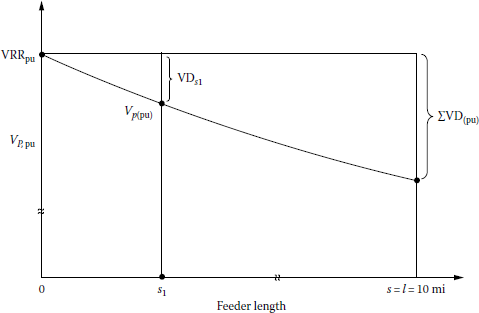
- When VP,pu = 1.010 pu V, the associated voltage drop at the distance s1, as shown in Figure 9.14, is
From Example 9.1, the total voltage drop of the feeder is
Therefore, the distance sl can be found from the following parabolic formula for the uniformly distributed load:
or
from which the following quadratic equation can be obtained:
which has two solutions, namely, 1.75 and 18.23 mi. Therefore, the distance s1, taking the acceptable answer, is 1.75 mi.
- When VP,pu = 1.00 pu V, the associated voltage drop at the distance s1 is
Therefore, from Equation 9.18,
or
which has two solutions, namely, 2.6 and 17.4 mi. Thus, taking the acceptable answer, the distance s1 is 2.6 mi.
- The advantage of part (a) over part (b) is that it can compensate for future growth. Otherwise, the VP, pu might be less than 1.00 pu V in the future.
Example 9.3
Assume that the peak-load primary-feeder voltage at the input to the regulator is 1.010 pu V as given in Example 9.2. Determine the necessary minimum kilovoltampere size of each of three single-phase feeder regulators.
Solution
From Example 9.2, the distance s1 is found to be 1.75 mi. Previously, the annual peak load and the standard regulation range have been given as 4000 kVA and ±10%, respectively.
The uniformly distributed three-phase load at s1 is
Therefore, the single-phase load at s1 is
Since the single-phase regulator kilovoltampere rating is given by
where Sckt is the circuit kilovoltamperage, then
Thus, from Table 9.3, the corresponding minimum kilovoltampere size of the regulator size can be found as 114.3 kVA.
Example 9.4
Use the distance of s1 = 1.75 mi found in Example 9.2 and assume that the distance of the RP is equal to s1, that is, sRP = s1, or, in other words, the RP is located at the regulator station, and determine the following:
- Specify the best settings for the LDC’s R and X, and for the VRR.
- Sketch voltage profiles for zero load and for the annual peak load. Label significant voltage values on the curves.
- Are the primary-feeder voltage (VP,pu) criteria met?
Solution
- The xRP = s1 means that the RP is located at the feeder regulator station. Therefore, the best settings for the LDC of the regulator are when settings for both R and X are zero and
- The voltage drop occurring in the feeder portion between the RP and the end of the feeder is
Thus the primary-feeder voltage at the end of the feeder for the annual peak load is
Note that the VP,pu used at the regulator point is the no-load value rather than the annual peak-load value. If, instead, the 1.0667 pu value is used, then, for example, television sets of those customers located at the vicinity of the RP might be damaged during the off-peak periods because of the too-high VRP value.
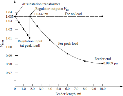
As can be seen from Figure 9.15, the peak-load voltage profile is not in linear but in parabolic shape. The voltage-drop value for any given point s between the substation and the regulator station can be calculated from
where
- K is the percent voltage drop per kilovoltampere-mile characteristic of feeder
- S3ϕ is the uniformly distributed three-phase annual peak load, kVA
- ℓ is the primary feeder length, mi
- s is the distance from substation, mi
Therefore, from Equation 9.20,
For various values of s, the associated values of the voltage drops and VP,pu can be found, as given in Table 9.4.
For Annual Peak Load
s (mi)
VDs (pu V)
Vp,pu (pu V)
0.0
0.0
1.035
0.5
0.0076
1.0274
1.0
0.0071
1.0203
1.5
0.0068
1.0135
1.75
0.025
1.010
The voltage-drop value for any given point s between the substation and the regulator station can also be calculated from
where
IL is the load current in feeder at substation end
r is the resistance of feeder main, Ω/mi per phase
x is the reactance of feeder main, Ω/mi per phase
Therefore, the voltage drop in per units can be found as
The voltage-drop value for any given point s between the regulator station and the end of the feeder can be calculated from the following equation:
where = uniformly distributed three-phase annual peak load at distance s1, kVA
s1 is the distance of feeder regulator station from substation, mi Therefore, from Equation 9.25,
For various values of s, the corresponding values of the voltage drops and VP,pu can be found, as given in Table 9.5.
For Annual Peak Load
s (mi)
VDs (pu V)
Vp,pu (pu V)
0.00
0.00
1.0337
0.75
0.0092
1.0245
2.25
0.0157
1.0088
4.25
0.0155
0.9933
6.25
0.0093
0.9840
8.25
0.0031
0.9809
The voltage profiles for the annual peak load can be obtained by plotting the VP,pu values from Tables 9.4 and 9.5. Since there is no voltage drop at zero load, the VP,pu remains Constant at 1.035 pu. Therefore, the voltage profile for the zero load is a horizontal line (with zero slope
- The minimum VP,pu criterion of 1.0083 pu V is not met even though the regulator voltage has been set as high as possible without exceeding the maximum voltage criterion of 1.035 pu V.
Example 9.5
Assume that the regulator station is located at a distance sl as found in part (a) of Example 9.2, but the RP has been moved to the end of the feeder so that sRP = I = 10 mi.
- Determine good settings for the values of VRR, R, and X so that all VP,pu voltage criteria will be met, if possible.
- Sketch voltage profiles and label the values of significant voltages, in per unit volts.
Solution
- From Table A.4 of Appendix A, the resistance at 50°C and the reactance of the 266.8 kcmil AAC with 37 strands are 0.386 and 0.4809 Ω/mi, respectively. From Table A.10, the inductive-reactance spacing factor for the 53-in geometric mean spacing is 0.1802 Ω/mi. Therefore, from Equation 9.6, the inductive reactance of the feeder conductor is
From Equations 9.3 and 9.5,
and
From Table 9.3, for the regulator size of 114.3 kVA found in Example 9.3, the primary rating of the CT and the PT ratio are 150 and 63.5, respectively. Therefore, from Equations 9.2 and 9.4, the R and X dial settings can be found as
based on 120 V and
Assume that the voltage at the RP (VRP) is arbitrarily set to be 1.0138 pu V using the R and X settings of the LDC of the regulator so that the VRP is always the same for zero load or for the annual peak load. Therefore, the output voltage of the regulator for the annual peak load can be found from
Here, note that the regulator regulates the regulator output voltage automatically according to the load at any given time in order to maintain the RP voltage at the predetermined voltage value.
Table 9.6 gives the VP,pu values for the purpose of comparing the actual voltage values against the established voltage criteria for the annual peak and for zero load.
Actual Voltages vs. Voltage Criteria at Peak and Zero Loads
Actual Voltage (pu V)
Voltage Criteria (pu V)
Voltage
At Peak Load
At Zero Load
At Peak Load
At Zero Load
Max VP,pu
1.0666
1.0138
1.0667
1.0337
Min VP,pu
1.0138
1.0138
1.0083
1.0083
Values Obtained
s (mi)
VDs (pu V)
VP,pu (pu V)
0.00
0.00
1.0666
0.75
0.0092
1.0574
2.25
0.0157
1.0417
4.25
0.0155
1.0262
6.25
0.0093
1.0169
8.25
0.0031
1.0138
As can be observed from Table 9.6, the primary voltage criteria are met by using the R and X settings.
- The voltage profiles for the annual peak load and zero load can be obtained by plotting the VP,pu values from Tables 9.6 and 9.7 (based on Equation 9.26), as shown in Figure 9.16.
Example 9.6
Consider the results of Examples 9.4 and 9.5 and determine the following:
- The number of steps of buck and boost the regulators will achieve in Example 9.4.
- The number of steps of buck and boost the regulators will achieve in Example 9.5.
Solution
- For Example 9.4, the number of steps of buck is
thus it is either zero or one step. The number of boost is
therefore it is either three or four steps.
- For Example 9.5, the number of steps of buck is
hence, it is either three or four steps. The number of steps of boost is
therefore, it is either 9 or 10 steps.
Example 9.7
Consider the results of Examples 9.4 and 9.5 and answer the following:
- Can reduced range of regulation be used gainfully in Example 9.4? Explain.
- Can reduced range of regulation be used gainfully in Example 9.5? Explain.
Solution
- Yes, the reduced range of regulation can be used gainfully in Example 9.4 since the next-smaller-size regulator, that is, 76.2 kVA, at ±5% regulation range can be selected. This ±5% regulation range would allow the capacity of the regulator to be increased to 160% (see Table 9.2) so that
which is much larger than the required capacity of 110 kVA. It would allow the user ±8 steps of buck and boost, which is more than the required one step of buck and four steps of boost.
- No, the reduced range of regulation cannot be used gainfully in Example 9.5 since the required steps of buck and boost are 4 and 10, respectively. The reduced range of regulation at ±6.25% would provide the ±10 steps of buck and boost, but it would allow the capacity of the regulator to be increased only up to 135% (see Table 9.2) so that
which is smaller than the required capacity of 110 kVA.
Example 9.8
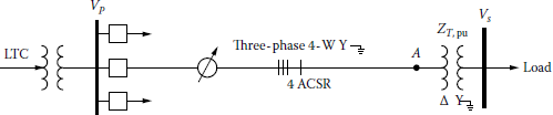
Figure 9.17 shows a one-line diagram of a primary feeder supplying an industrial customer. The nominal voltage at the utility substation low-voltage bus is 7.2/13.2 kV three-phase wye-grounded. The voltage regulator bank is made up of three single-phase step-type voltage regulators with a PT ratio of 63.5 (7620:120).
The industrial customer’s bus is located at the end of a 3 mi primary line with a resistance of 0.30 Ω/mi and an inductive reactance of 0.80 Ω/mi.
The customer’s transformer is rated 5000 kVA in three phase with a 12,800 V primary connected in delta (taps in use) and a 2400/4160 V secondary connected in grounded-wye. The transformer impedance is 0 + j0.05 pu Ω based on the rated kilovoltamperes and tap voltages in use. Assume that the bases to be used are 5,000 kVA, 2,400/4,160 V, and 7,390/12,800 V.
Assume that the customer asks that the low-voltage bus be regulated to 2450/4244 V and determine the following:
- Find the necessary setting of the voltage-setting dial of the VRR of each single-phase regulator in use.
- Assume that the ratio of the CT in each regulator is 250:1 A and find the necessary R and X dial settings of LDCs.
Solution
- The voltage at the RP, which is located at the customer’s bus, is
Therefore,
Thus,
or, alternatively,
- The applicable impedance base is
therefore, the transformer impedance is
Since here the R and X settings are determined for only one customer, the resistance and reactance values of the customer’s transformer have to be included in the effective resistance and reactance calculations. Therefore,
and
Thus, the R dial setting of the LDC is
and the X dial setting is
Example 9.9
Consider the 10 mi feeder of Example 9.1. Assume that the substation has a bus voltage regulator (BVR) with transformer LTC and that the primary feeder voltage (VP) has been set on the VRR to be 1.035 pu V.
Assume that the main feeder is made up of 266.8 kcmil with 37 strands and 53-in geometric mean spacing. It has been found in Example 9.5 that the main feeder has an inductive reactance of 0.661 Ω/mi per conductor. Assume that the annual peak load is 4000 kVA at a lagging power factor of 0.85 and distributed uniformly along the main or, in other words, the uniformly distributed load is
Assume that, as found in Example 9.1, the total voltage drop of the feeder is
and the reactive load factor is 0.40. Use the given data and determine the following:
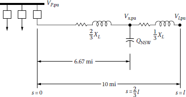
- Design a fixed, that is, nonswitched (NSW)-capacitor bank for the maximum loss reduction.
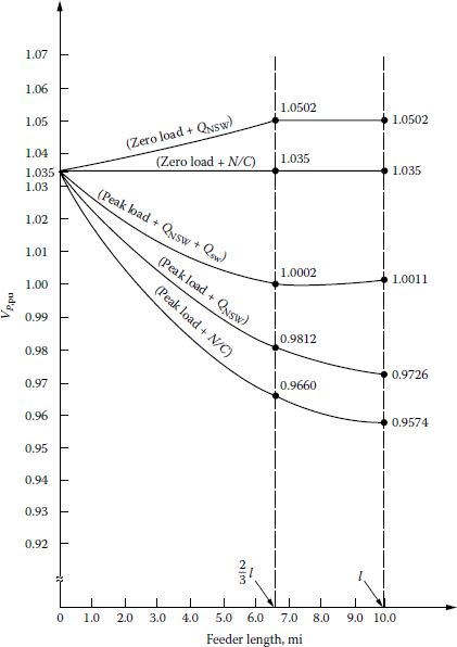
- Sketch the voltage profiles when there is no-capacitor (N/C) bank installed and when there is a fixed-capacitor bank, that is, QNSW installed.
- Add a switched-capacitor bank for voltage control on the feeder. Locate the switched-capacitor bank, that is, Qsw, at the end of the feeder for the feeder at the annual peak load is 1.000 pu V. Sketch the associated voltage profiles.
Solution
- From Figure 8.31, the corrective ratio (CR) for the given reactive load factor of 0.40 is found to be 0.27. Therefore, the required size of the NSW-capacitor bank is
Thus, two single-phase standard 100-kvar-size capacitor units are required to be used on each phase and located on the feeder at a distance of
for the optimum result, as shown in Figure 9.18.
Therefore, the per unit voltage rise (VRPpu) due to the NSW-capacitor bank is
- When there is N/C bank installed, the voltage drop for the uniformly distributed load at a distance of s = 2/3 ℓ can be found from Equation 9.18 as
or
from which
Therefore, the feeder voltage at the 2/3 l distance is
When there is a fixed-capacitor bank installed, the new voltage at the 2/3 l distance due to the voltage rise is
When there is N/C bank installed, the voltage at the end of the feeder is
When there is a fixed-capacitor bank installed, the new voltage at the end of the feeder due to the voltage rise is
The associated voltage profiles are shown in Figure 9.19.
- Since the new voltage at the end of the feeder due to the Qsw installation is 1.000 pu V at the annual peak load, the required voltage rise is
Therefore, the required size of the switched-capacitor bank can be found from
or
Hence, the possible combinations of the single-phase standard-size capacitor units to make up the capacitor bank are
- Fifteen single-phase standard 50 kvar capacitor units, for a total of 750 kvar
- Six single-phase standard 100 kvar capacitor units, for a total of 600 kvar
- Nine single-phase standard 100 kvar capacitor units, for a total of 900 kvar For example, assume that the first combination, that is,
is selected. The resultant new voltage rises at the distance of I and s = s = 2/3 ℓ are
and
Therefore, at the peak load when both the NSW- (i.e., fixed) and the switched-capacitor banks are on, the voltage at two-thirds of the line and at the end of the line are
and
respectively. At zero load when there is N/C bank installed, the voltages at two-thirds of the line and at the end of the line are the same and equal to 1.035 pu V. The associated voltage profiles are shown in Figure 9.19.
Example 9.10
Consider Example 9.8 and assume that the industrial load at the annual peak is 5000 kVA at 80% lagging power factor. Assume that the customer wishes to add some additional load, is currently paying a monthly power-factor penalty, and the single-phase voltage regulators are approaching full boost. Select a proper three-phase capacitor-bank size (in terms of the multiples of three-phase 150 kvar capacitor units) to be connected to the 4 kV bus that will (1) produce a voltage rise of at least 0.020 pu V on the 4 kV bus and (2) raise the on-peak power factor of the present load to at least 88% lagging power factor.
Solution
The presently existing load is
or
at 80% lagging power factor. When a properly sized capacitor bank is connected to the bus to improve the on-peak power factor to 88%, the real power portion will be the same but the reactive power portion will be different. In other words,
from which
therefore
and hence the magnitude of the new apparent power is
Therefore, the minimum size of the capacitor bank required to raise the load power factor to 0.88 is
Thus, if a 900-kvar-capacity bank is used, the resultant voltage rise from Equation 9.39 is
where
hence
which is larger than the given voltage-rise criterion of 0.020 pu V. Therefore, it is proper to install six 150 kvar three-phase units as the capacitor bank to meet the criteria.
9.6 Distribution Capacitor Automation
Today, intelligent customer meters can now monitor voltage at key customer sites and communicate this information to the utility company. Thus, system information can be fine-tuned based on the actual measured values at the end point, rather than on projected values, combined with var information integrated into the control scheme.
The distributed capacitor automation takes advantage of distributed-processing capabilities of electronic meters, capacitor controllers, radios, and substation processors. It uses an algorithm to switch field and substations’ capacitors on and off remotely, using voltage information from meters located at key customer sites, and var information from the substation, as illustrated in Figure 9.20.
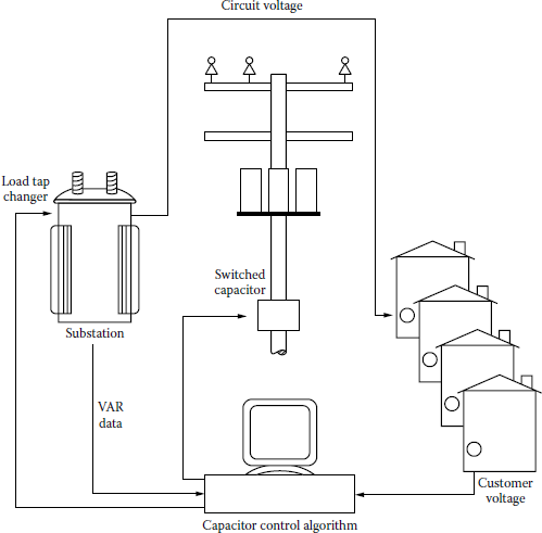
A distribution capacitor automation algorithm switches capacitors on and off remotely and automatically, using voltage information from customer meters and var information from the substation.
In the past, capacitors on distribution system were switched on and off mainly by stand-alone controllers that monitored circuit voltage at the capacitor. Various control strategies, including temperature and/or time bias settings on capacitor controllers, were used to ensure operation during predicted peak loading conditions. While this system provided adequate peak voltage/var support, it necessarily involved overcompensation to ensure that all customers were receiving adequate voltage service. Also, capacitors operated independently and were not integrated into a system-wide control scheme.
Distribution capacitor automation integrates field and substation capacitors into a closed-loop control scheme, within a structure that operates as follows:
- Intelligent customer meters provide exception reporting on voltages out of set BWs. They also report 5-min average voltages when polled.
- Meters communicate via power-line carrier to the nearest packed radio, and via radio-frequency packet communication, to the designed capacitor controller.
- Each capacitor controller-automation programmed to receive meter voltages (received from several meters) to a substation processor.
- The distribution capacitor automation program algorithm, running on an industrial-grade processor at the substation, determines the optimal capacitor-switching pattern and communicates control instructions to capacitor controllers.
Customer meters are strategically placed to provide a consistent sample of lower voltage customers. The system aims to maintain every customer’s voltage within a tighter BW targeted at a minimum of 114 V.
Substation reactive power flow is optimized by using control BW set points in the processor. For example, the operator may set a desired power factor as measured at the substation transformer, and the algorithm would act accordingly, choosing the pattern of capacitor switching to both maintain minimum customer voltage and at the same time meet the substation var requirements. In cases where distribution substations have load-tap changing (LTC) transformers, the control algorithm calculates optimal bus voltage in order to produce unity power factor, and the processor issues commands to the LTC controller to hold to this optimal voltage level [19].
To control subtransmission reactive power flow, the transmission substation processor interfaces with distribution substation processors to derive a subtransmission voltage level for minimum var flow and customer voltages.
9.7 Voltage Fluctuations
In general, voltage fluctuations and lamp flicker on distribution systems are caused by a customer’s utilization apparatus. Lamp flicker can be defined as a sudden change in the intensity of illumination due to an associated abrupt change in the voltage across the lamp. Most flickers are caused by the starting of motors. The large momentary inrush of starting current creates a sudden dip in the illumination level provided by incandescent and/or fluorescent lamps since the illumination is a function of voltage.
Therefore, a utility company tries not to endanger other customers, from the quality-of-service point of view, in the process of serving a new customer who could generate excessive flicker by the company’s standards. Thus, the distribution circuits are checked to determine whether or not the flicker caused by the new customer’s load in addition to the existing flicker-generating loads will meet the company’s voltage-fluctuating standards.
The decision to serve such a customer is based on the load location, load type, service voltage, frequency of the motor starts, the motor’s horsepower rating, and the motor’s NEMA code considerations. Momentary, or pulsating, loads are considered for both their starting requirements and the change in power requirements per unit time. Often, more severe flickers result due to the running operation of pulsating loads than the starting loads. Usually, the pulsating loads, such as grinders, hammer mills, rock crushers, reciprocating pumps, and arc welders, require additional study.
The annoyance created by lamp flicker is a very subjective matter and differs from person to person. However, in certain cases, the flicker can be very objectionable and can create great discomfort. In general, the degree of objection to lamp flicker is a function of the frequency of its occurrence and the rate of change of the voltage dip. The voltage changes resulting in lamp flicker can be either cyclic or noncyclic in nature. Usually, cyclic flicker is more objectionable.
Figure 9.21 shows a typical curve used by the utilities to determine the amount of voltage flicker to be allowed on their system. As indicated in the figure, flicker values located above the curve are likely to be objectionable to lighting customers. For example, from the figure, it can be observed that 5 V dips, based on 120 V, are satisfactory to lighting customers as long as the number of dips does not exceed 3/h.
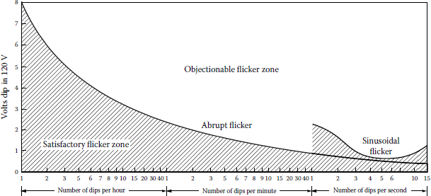
Thus, more frequent dips of this magnitude are in the objectionable-flicker zone, that is, they are objectionable to the lighting customers. The curve for sinusoidal flicker should be used for the sinusoidal voltage change caused by pump compressors and equipment of similar characteristics. Each utility company develops its own voltage-flicker-limit curve based on its own experiences with customer complaints in the past.
Distribution engineers strive to keep voltage flickers in the satisfactory zone by securing compliance with the company’s flicker standards and requirements, and by designing new extensions and rebuilds that will provide service within the satisfactory-flicker zone. Flicker due to motor starting can be reduced by the following remedies:
- Using a motor that requires less kilovoltamperes per horsepower to start
- Choosing a low-starting-torque motor if the motor starts under light load
- Replacing the large-size motor with a smaller-size motor or motors
- Employing motor starters to reduce the motor inrush current at the start
- Using shunt or series capacitors to correct the power factor
As mentioned at the start of this section, distribution engineers try every reasonable means to satisfy the motor-start flicker requirement. After exhausting other alternatives, they may choose to satisfy the flicker condition by installing shunt or series capacitors.
Shunt capacitors compensate for the low power factor of the motor during start. They are removed from the circuit when the motor reaches nominal running speed. At start and for a very short time, not to exceed 10 s, capacitors rated at line-to-neutral voltage are often connected line-to-line, that is, at a voltage greater than their rating by a factor of . Thus, the momentary effective kilovar rating of the capacitors becomes equal to three times the rated kilovars since (VL–L/VL–N)2 = 3.
If series capacitors are used, they should be installed between the substation transformer and the residential or lighting tap, as shown in Figure 9.22. Installing the capacitor between the residential load and the fluctuating load would not reduce the flicker voltage since it would not reduce the impedance between the source and the lighting bus.
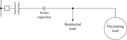
Installation of series capacitor to reduce the flicker voltage caused by a fluctuating load.
Since series capacitors are permanently installed in the primary feeder, they require special devices to protect them against overvoltage and resonance conditions. Therefore, a typical series-capacitor installation costs three or four times as much as shunt-motor-start capacitors. Series capacitors correct the power factor of the system, not the motor. The position of the series capacitors in the circuit is especially important if there are other customers along the line.
9.7.1 Shortcut Method to Calculate the Voltage Dips due to a Single-Phase Motor Start
If the starting kilovoltamperage of a single-phase motor is known, the motor’s starting current can be found as
and the voltage dip based on 120 V can be calculated from
where
Substituting Equations 9.45 and 9.47 into Equation 9.46, the voltage dip can be expressed as
where
- VDIP is the voltage dip due to single-phase motor start expressed in terms of 120 V base, V Sstart is the starting kVA of single-phase motor, kVA
- If,L–G is the line-to-ground fault current available at point of installation and obtained from fuse coordination, A
- VL–N is the line-to-neutral voltage, kV
Example 9.11
Assume that a 10-hp single-phase 7.2 kV motor with NEMA code letter “G” starting 15 times per hour is to be served at a certain location. If the starting kilovoltamperes per horsepower for this motor is given by the manufacturer as 6.3, and the line-to-ground fault at the installation location calculated to be 1438 A, determine the following:
- The voltage dip due to the motor start, in volts
- Whether or not the resultant voltage dip is objectionable
Solution
- Since the starting kilovoltamperes per horsepower is given as 6.3, the starting kilovoltamperes can be found as
Therefore, the voltage dip due to the motor start, from Equation 9.48, can be calculated as
- From Figure 9.21, it can be found that the voltage dip of 0.73 V with a frequency of 15 times/h is in the satisfactory-flicker zone and therefore is not objectionable to the immediate customers.
9.7.2 Shortcut Method to Calculate the Voltage Dips due to a Three-Phase Motor Start
If the starting kilovoltamperes of a three-phase motor is known, its starting current can be found as
and the voltage dip based on 120 V can be calculated from
where
Substituting Equations 9.50 and 9.52 into Equation 9.51, the voltage dip can be expressed as
where
- VDIP is the voltage dip due to three-phase motor start expressed in terms of 120 V base, V Sstart is the starting kVA of three-phase motor, kVA
- I3ϕ is the three-phase fault current available at the point of installation and obtained from fuse coordination, A
- VL–L is the line-to-line voltage, kV
Example 9.12
Assume that a 100-hp three-phase 12.47 kV motor with NEMA code letter "F" starting three times per hour is to be served at a certain location. If the starting kilovoltampere per horsepower for this motor is given by the manufacturer as 5.6, and the three-phase fault current at the installation location calculated to be 1765 A, determine the following:
- The voltage dip due to the motor start
- Whether or not the resultant voltage dip is objectionable
Solution
- Since the starting kilovoltampere per horsepower is given as 5.6, the starting kilovoltampere can be found from Equation 9.49 as
Therefore, the voltage dip due to the motor start, from Equation 9.53, can be calculated as
- From Figure 9.21, it can be found that the voltage dip of 1.72 V with a frequency of three times per hour is in the satisfactory-flicker zone and therefore is not objectionable to the immediate customers.
Problems
- 9.1 Derive, or prove, Equation 9.18.
- 9.2 Derive, or prove, Equation 9.20.
- 9.3 Repeat Example 9.1, assuming 336.4 kcmil ACSR conductors and annual peak load of 5000 kVA at a lagging-load power factor of 0.90.
- 9.4 Repeat Example 9.2, assuming 336.4 kcmil ACSR conductors and annual peak load of 5000 kVA at a lagging-load power factor of 0.90.
- 9.5 Repeat Example 9.3, assuming 336.4 kcmil ACSR conductors and annual peak load of 5000 kVA at a lagging-load power factor of 0.90.
- 9.6 Repeat Example 9.4, assuming 336.4 kcmil ACSR conductors and annual peak load of 5000 kVA at a lagging-load power factor of 0.90.
- 9.7 Repeat Example 9.5, assuming 336.4 kcmil ACSR conductors and annual peak load of 5000 kVA at a lagging-load power factor of 0.90.
- 9.8 Repeat Example 9.6, assuming 336.4 kcmil ACSR conductors and annual peak load of 5000 kVA at a lagging-load power factor of 0.90.
- 9.9 Assume that a subtransmission line is required to be designed to carry a contingency peak load of 2 × SIL. A 60% series compensation is to be used, that is, the capacitive reactance (Xc) of the capacitor bank required to be installed is equal to 60% of the total series inductive reactance per phase of the transmission line. Assume that each phase of the series-capacitor bank is to be made up of series and parallel groups of two-bushing 12 kV 150 kvar shunt power-factor-correction capacitors. Assume that the three-phase SIL of the line is 416.5 MVA and its inductive line reactance is 117.6 Ω/phase. Specify the necessary series–parallel arrangement of capacitors for each phase.
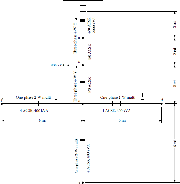
- 9.10 In this problem, design improvements of the designer choice to correct the undervoltage conditions are investigated on the radial system shown in Figure P9.10.
The voltage at the distribution substation low-voltage bus is kept at 1.04 pu V with bus-voltage regulation. The per unit voltages at annual peak-load values at the points a, b, c, d, e, and f are 1.0049, 0.9815, 0.9605, 0.8793, 0.8793, and 0.8793, respectively. Use the nominal operating voltage of 7,200/12,470 V of the three-phase four-wire wye-grounded system as the base voltage. Assume that all given kilovoltampere loads are annual peak values at 85% lagging-load power factor. The load between the substation bus and point a is a uniformly distributed load of 2000 kVA. The loads on the laterals c, d, c–e, and c–f are also uniformly distributed, each with 400 kVA. There is a lumped load of 800 kVA at point b .
The line data for the #4/0 and 4 ACSR conductors are given in Table P9.10.
Table for Problem P9.10
Conductor Size
R, Ω/(phase · mi)
X, Ω/(phase · mi)
K, pu VD/(kVA · mi)
4/0
0.592
0.761
5.85 × 10⁻⁶
4
2.55
0.835
1.69 × 10⁻⁵
To improve voltage conditions, consider any or all combinations of the following design remedies:
- Installation of shunt capacitor bank(s)
- Installation of 32-step voltage regulators with a maximum regulation range of ±10%
- Addition of new phase conductors
Using these remedies attempt to meet the following primary-voltage criteria:
- Maximum primary voltage must be 1.040 pu V at zero load.
- Maximum primary voltage must be 1.07 pu V at peak load.
- Minimum primary voltage must be 1.00 pu V at peak load.
If the installation of the capacitor alternative is chosen, determine the following:
- The rating of the capacitor bank(s) in three-phase kilovars.
- The location of the capacitor bank(s) on the given system.
- Whether or not voltage-controlled automatic switching is required.
If the installation of the voltage-regulator alternative is chosen, determine the following:
- The location of the regulator bank(s)
- The standard kilovoltampere rating of each single-phase regulator
- The location of the RP on the system
- The setting of the voltage-regulating relay (VRR)
- The R and X settings of the LDC
- 9.11 Repeat Example 9.9. Assume that the annual peak load is 5000 kVA at a lagging power factor of 0.80 and that the reactive load factor is 0.60.
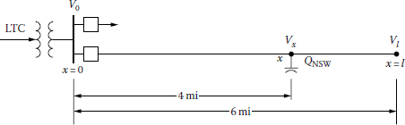
- 9.12 Figure P9.12 shows an open-wire primary line with many laterals and uniformly distributed load. The voltage at the distribution substation low-voltage bus is held at 1.03 pu V with BVR. When there is N/C bank installed on the feeder, that is, QNSW = 0, the per unit voltage at the end of the line at annual peak load is 0.97. Use the nominal operating voltage of 7.97/13.8 kV of the three-phase four-wire wye-grounded system as the base voltage. Assume that the off-peak load of the system is about 25% of the on-peak load. Also assume that the line reactance is 0.80 Ω/(phase · mi), but the line resistance is not given and determine the following:
- When the shunt-capacitor bank is not used, find the Vx voltages at the times of peak load and off-peak load.
- Apply an NSW-capacitor bank and locate it at the point of x = 4 mi on the line, and size the capacitor bank to yield the per unit voltage of 1.05 at point x at the time of zero load. Find the size of the capacitor (QNSW) in three-phase kilovars. Also find the per unit voltage of Vx and V1 at the time of peak load.
- 9.13 Figure P9.13 shows a system that has a load connected at the end of a 3.5 mi #4 ACSR open-wire primary line. The load belongs to an important scientific equipment installation, and it varies from nearly zero to 1000 kVA. The load requires a closely regulated voltage
at the Vs bus. The consumer requests the voltage Vs to be equal to 1.000 ± 0.010 pu and offers to compensate properly the supplying utility company for such high-quality voltage-regulated service.
A junior engineer proposes to build the 3.5 mi #4 ACSR line to a nearby distribution substation and to place the feeder voltage regulators there in order to render the service requested. His wire size is generous for ampacity. He proposes a BW setting of ±1.0 V based on 120 V.
There is BVR at the substation, but at times the BVR equipment is disconnected and bypassed for maintenance and repair. Therefore, the substation bus voltage VP,pu is as follows. When BVR is in use,
When BVR is out,
The nominal and base voltage at the distribution substation low-voltage bus is 7,200/12,470 V for the three-phase four-wire wye-grounded system. The nominal and base voltage at the consumer’s bus is 277/480 V for the three-phase four-wire wye-grounded service. Assume that the regulator bank is made up of three single-phase 32-step feeder voltage regulators with ±10% regulation range. The feeder impedance is given as 2.55 + j0.835 Ω/(mi × phase). Assume that the precalculated K constant of the line is 1.69 x10⁻⁵ pu VD/(kVA × mi) at 85% power factor. The consumer’s transformer is rated as 1000 kVA, three phase, with 12,470 V high-voltage rating. It has an impedance of 0 + j0.055 pu based on the transformer ratings.
Using the given information and data, determine and state whether or not the young engineer’s proposed design will meet the consumer’s requirements. (Check for both cases, that is, when BVR is in use and BVR is not in use.)
- 9.14 Repeat Example 9.11, assuming 20 starts per hour and a line-to-ground current of 350 A.
- 9.15 Repeat Example 9.12, assuming 10 starts per hour and a three-phase fault current of 750 A.
- 9.16 Resolve parts (a) and (b) of Example 9.1 by using MATLAB. Assume that all the quantities remain the same.
References
1. Westinghouse Electric Corporation: Electric Utility Engineering Reference Book-Distribution Systems, Vol. 3, Westinghouse Electric Corporation, East Pittsburgh, PA, 1965.
2. ANSI C84.1-1977: Voltage Ratings for Electric Power Systems and Equipment, American National Standards Institute.
3. McCrary, M. R.: Regulating voltage on a major power system, The Line, 81(1), 1981, 2–8.
4. Hopkinson, R. H.: Recap $ computer program aids voltage regulation studies. Electr. Forum. 4(4), 1978, 20–23.
5. Fink, D. G. and H. W. Beaty: Standard Handbook for Electrical Engineers, 11th edn., McGraw-Hill, New York, 1978.
6. Gönen, T. et al.: Development of AdvancedMethods for Planning Electric Energy Distribution Systems, U.S. Department of Energy, October 1979. Available from the National Technical Information Service, U.S. Department of Commerce, Springfield, VA.
7. Oklahoma Gas and Electric Company: Engineering Guides, Oklahoma Gas and Electric Company, Oklahoma City, OK, January 1981.
8. Bovenizer, W. N.: New ‘Simplified’ regulator for lower-cost distribution voltage regulation, The Line, 75(1), 1975, 25–28.
9. Bovenizer, W. N.: Paralleling voltage regulators, The Line, 75(2), 1975, 6–9.
10. Sealey, W. C.: Increased current ratings for step regulators, AIEE Trans., 74(pt. III), August 1955, 737–742.
11. Lokay, H. E. and D. N. Reps: Distribution system primary-feeder voltage control: Part I-A new approach using the digital computer, AIEE Trans., 77(pt. III), October 1958, 845–855.
12. Reps, D. N. and G. J. Kirk, Jr.: Distribution system primary-feeder voltage control: Part II-digital computer program, AIEE Trans., 77(pt. III), October 1958, 856–865.
13. Amchin, H. K., R. J. Bentzel, and D. N. Reps: Distribution system primary-feeder voltage control: Part III-computer program application, AIEE Trans., 77(pt. III), October 1958, 865–879.
14. Reps, D. N. and R. F. Cook: Distribution system primary-feeder voltage control: Part IV-A supplementary computer program for main-circuit analysis, AIEE Trans., 78(pt. III), October 1958, 904–913.
15. Chang, N. E.: Locating shunt capacitors on primary feeder for voltage control and loss reduction, IEEE Trans. Power Appar. Syst., PAS-88(10), October 1969, 1574–1577.
16. Gönen, T. and F. Djavashi: Optimum shunt capacitor allocation on primary feeders, IEEE MEXICON-80 International Conference, Mexico City, Mexico, October 22–25, 1980.
17. Ku, W. S.: Economic comparison of switched capacitors and voltage regulators for system voltage control, AIEE Trans., 76(pt. III), December 1957, 891–906.
18. Gönen, T. and F. Djavashi: Optimum loss reduction from capacitors installed on primary feeders, The Midwest Power Symposium, Purdue University, West Lafayette, IN, October 27–28, 1980.
19. Williams, B.R. and D.G. Walden: Distribution automation strategy for the future, IEEE Comp. Appl. Power, 7(3), July 1994, 16–21.