Chapter 13
Distributed Generation and Renewable Energy
Simplicity is the most deceitful mistress that ever betrayed man.
Henry Brooks Adams
It was involuntary. They sank my boat.
John F. Kennedy. 1965 (Remark when asked how he become a hero.)
13.1 Introduction
Renewable energy is of many types, including wind, solar, hydro, geothermal (earth heat), and biomass (waste material). All renewable energy with the exception of tidal and geothermal power, and even the energy of fossil fuels, ultimately comes from the sun. About 1%–2% of energy coming from the sun is converted into wind energy. Today, the most prevalent renewable energy resources are wind and solar that will be reviewed briefly in this chapter.
13.2 Renewable Energy
Renewable energy* is also a naturally distributed resource, that is, it can provide energy to remote areas without the requirement for elaborate energy transportation systems. However, it needs to be pointed out that it is not always a requirement that the renewable energy has to be converted into electricity. Solar water heating and wind-powered water pumping are good examples for it.
Presently, the largest renewable energy technology application (with the exception of hydro) has taken place is wind power, with 95 GW, worldwide by the end of 2007. In 2003, renewable energy contributed 13.5% of the world’s total primary energy (2.2% hydro, 10.8% combustible renewables and waste, and 0.5% geothermal, solar, and wind). Even though the combustible renewables are used for heat, the contributions for electric generation were somewhat different: hydro contributed 15.9% and geothermal, solar, wind, and combustibles contributed 1.9%.
The capacity of the world’s hydro plant is over 800 GW, and the capacity of fast-developing wind energy has sustained a 25% compound growth for well over a decade and was about 60 GW by the end of 2005. Also, in 2003, the world’s electricity production from hydro was about 2654 TWh and all other renewables provided 310 TWh.
It is known that the world’s primary energy demand almost doubled between 1971 and 2003. Furthermore, it is projected to increase by another 40% by 2020. It is also known that in the last 30 years, there has been a considerable shift away from oil and toward the natural gas. The natural gas accounted for 21% of primary energy and 19% of electricity generation, worldwide, in 2003. The impetus for this change has primarily been the increasing concerns over global warming due to carbon dioxide emissions.
13.3 Impact of Dispersed Storage and Generation
Following the oil embargo and the rising prices of oil, the efforts toward the development of alternative energy sources (preferably renewable resources) for generating electric energy have been increased. Furthermore, opportunities for small power producers and cogenerators have been enhanced by recent legislative initiatives, for example, the Public Utility Regulatory Policies Act (PURPA) of 1978, and by the subsequent interpretations by the Federal Energy Regulatory Commission (FERC) in 1980.
The following definitions of the criteria affecting facilities under PURPA are given in Section 201 of PURPA:
- A small power production facility is one that produces electric energy solely by the use of primary fuels of biomass, waste, renewable resources, or any combination thereof. Furthermore, the capacity of such production sources together with other facilities located at the same site must not exceed 80 MW.
- A cogeneration facility is one that produces electricity and steam or forms of useful energy for industrial, commercial, heating, or cooling applications.
- A qualified facility is any small power production or cogeneration facility that conforms to the previous definitions and is owned by an entity not primarily engaged in generation or sale of electric power.
In general, these generators are small (typically ranging in size from 100 kW to 10 MW and connectable to either side of the meter) and can be economically connected only to the distribution system, as shown in Figure 13.1. They are defined as dispersed storage and generation (DSG) devices. If properly planned and operated, DSG may provide benefits to distribution systems by reducing capacity requirements, improving reliability, and reducing losses. Examples of DSG technologies include hydroelectric and diesel generators, wind electric systems, solar electric systems, batteries, storage space and water heaters, storage air conditioners, hydroelectric pumped storage, photovoltaics (PVs), and fuel cells.

13.4 Integrating Renewables into Power Systems
Before going any further, it might be appropriate to define some terminologies including the terms grid, grid connected, and national grid. The term grid is usually used to describe the totality of the electric power network. The term grid connected means connected to any part of the power network. On the other hand, the term national grid usually means the extra-high voltage (EHV) transmission network.
The physical connection of a generator to the network is defined as integrated. But it is required that the necessary attention must be given to the secure and safe operation of the system and the control of the generator to achieve optimality in terms of the energy resource usage.
In general, the integration of the generators powered by the renewable energy sources essentially is the same as fossil fuel-powered generators and is based on the same methodology. However, renewable energy sources are very often variable and geographically dispersed.
A renewable energy generator can be defined as stand-alone or grid-connected. A stand-alone renewable energy generator provides for the greater part of the demand with or without other generators or storage. On the other hand, in a grid-connected system, the renewable energy generator supplies power to a large interconnected network that is also supplied power by other generators. Here, the power supplied by the renewable energy generator is only a small portion of the power supplied to the grid with respect to power supplied by other connected generators. The connection point is called the point of common coupling* (PCC).
13.5 Distributed Generation
It appears that there is a general consensus that by the end of this century the most of our electric energy will be provided by renewable energy sources. As said previously, small generators cannot be connected to the transmission system due to high cost of high-voltage transformers and switchgear.
Thus, small generators must be connected to the distribution system network. Such generation is known as distributed generation (DG) or dispersed generation. It is also called embedded generation since it is embedded in the distribution network.
Power in such power systems may flow from point to point within the distribution network. As a result, such unusual flow pattern may create additional challenges in the effective operation and protection of the distribution network.
Due to decreasing fossil fuel resources, poor energy efficiency, and environmental pollution concerns, the new approach for generating power locally at distribution voltage level by employing nonconventional/renewable energy sources such as natural gas, wind power, solar PV cells, biogas, cogeneration systems [which are combined heat and power (CHP) systems, Stirling engines, and microturbines.]
These new energy sources are connected to (or integrated into) the utility distribution network. As aforementioned, such power generation is called DG and its energy resources are known as distributed energy resources (DERs). Furthermore, the distribution network becomes active with the integration of DG and thus is known as active distribution network. The properties of DG include the following:
- It is normally less than 50 MW.
- It is neither centrally dispatched nor centrally planned by the power utility.
- The distributed generators or power sources are generally connected to the distribution systems, which typically have voltages of 240 V up to 34.5 kV.
The development and integration of the DG were based on the technical, economic, and environmental benefits that include the following:
- Reduction of environmental pollution and global warming concerns, as dictated by the Kyoto Protocol, and use of the nonconventional/renewable energy resources as a viable solution.
- As a result of rapid load growth, the fossil fuel reserves are increasingly depleted. Therefore, the use of nonconventional/renewable energy resources is increasingly becoming a requirement. Also, the use of DERs is to produce clean power without the associated pollution of the environment.
- DERs are usually modular units of small capacity because of their lower energy density and dependence on geographical conditions of a region.
- The overall power quality and reliability improves due to contributions of the stand-alone and grid-connected operations of DERs in generation augmentation. Such DG integration further increases due to deregulated environment and open access to the distribution network.
- The overall plant energy efficiency increases and also associated thermal pollution of the environment decreases because of the use of the DG such as cogeneration or CHP plants.
Furthermore, it is possible to connect a DER separately to the utility distribution network, or it may be connected as a microgrid due to the fact that the power is produced at low voltage. Thus, the microgrid can be connected to the utility’s network as a separate semiautonomous entity.
13.6 Renewable Energy Penetration
The proportion of electric energy or power being supplied from wind turbines or from other renewable energy sources is usually referred to as the penetration. It is usually given in percentage. The average penetration is defined by the following equation;
Average penetration=(Annual energy from renewableenergy powered generators(kWh))(Total annual energydelivered to loads(kWh))(13.1)
The term average penetration is used when fuel or CO2-emission savings are being considered.
However, for other purposes, including system control, use the following definition:
Instantaneous penetration=(Power from renewable energypowered generators (kW))(Power from renewable energypowered generators (kW)Total power deliveredto loads(kW))(13.2)
In general, the maximum instantaneous penetration is much greater than the average penetration.
13.7 Active Distribution Network
It is also called “generation embedded distribution network.” In the past, distribution networks had a unidirectional electric power transportation. That is, distribution networks were stable passive networks.
Today, the distribution networks are becoming active by the addition of DG that causes bidirectional power flows in the networks. Today’s distribution networks started to involve not only demand-side management but also integration of DG.
In order to have good active distribution networks that have flexible and intelligent operation and control, the following should be provided:
- Adaptive protection and control
- Wide-area active control
- Advanced sensors and measurements
- Network management apparatus
- Real-time network simulation
- Distributive penetrating communication network
- Knowledge and data extraction by intelligent methods
- New and modern design of transmission and distribution systems
13.8 Concept of Microgrid
A microgrid is basically an active distribution network and is made up of a collection of DG systems and various loads at distribution voltage level. They are generally small low-voltage combined heat loads of a small community. The examples of such small community include university or school campuses, a commercial area, an industrial site, a municipal region or a trade center, a housing estate, or a suburban locality.
The generators or microsources used in a microgrid are generally based on renewable/nonconventional distribution energy resources. They are integrated together to provide power at distribution voltage level. In order to introduce the microgrid to the utility power system as a single controlled unit that meets local energy demand for reliability and security, the microsources must have power electronic interfaces (PEIs) and controls to provide the necessary flexibility to the semiautonomous entity so that it can maintain the dictated power quality and energy output.
A microgrid is different than a conventional power plant. The differences include the following:
- Power generated at distribution voltage level and can thus be directly provided to the utility’s distribution system.
- They are of much smaller capacity with respect to the large generators in conventional power plants.
- They are usually installed closer to the customers’ locations so that the electric/heat loads can be efficiently served with proper voltage level and frequency and ignorable line losses.
- They are ideal for providing electric power to remote locations.
- The fundamental advantage of microgrids to a power grid is that they can be treated as a controlled entity within the power system.
- The fundamental advantage of microgrids to customers is that they meet the electric/heat requirements locally. This means that they can receive uninterruptable power, reduced feeder losses, improved local reliability, and local voltage support.
- The fundamental advantage to the environment is that they reduce environmental pollution and global warming by utilizing low-carbon technology.
However, before microgrids can be extensively established to provide a stable and secure operation, there are a number of technical, regulatory, and environmental issues that need to be addressed that include the establishment of standards and regulations for operating the microgrids in synchronism with the power utility, low energy content of the fuels involved, and the climate-dependent nature of the production of the DERs.
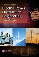
Figure 13.2 shows a microgrid connection scheme. Microgrid is connected to the medium voltage (MV) utility “main grid” through the PPC circuit breaker. Microsource and storage devices are connected to the feeders B and C through microsource controllers (MCs). Some loads on feeders B and C are considered to be priority loads (i.e., needing uninterruptable power supply), while the rest are non-priority loads. On the other hand, feeder B had only non-priority electric loads.
The microgrid has two modes of operations: (1) grid-connected and (2) stand-alone. In the first mode, the microgrid imports or exports power from or to the main grid. In the event of any disturbance in the main grid, the microgrid switches aver to stand-alone mode but still supply power to the priority loads. This is achieved by opening the necessary circuit breakers. But feeder A will be left alone so that it can ride through the disturbance.
The main functions of central controller (CC) include energy management module (EMM) and protection coordination module (PCM). The EMM supplies the set points for active and reactive power output, voltage, and frequency to each microgrid controller (MC). This is done by advanced communication and artificial intelligent techniques, whereas the PCM answers to microgrid and main grid faults and loss of grid situations so that proper protection coordination of the microgrid is achieved.
Chowdhuri et al. [1] define the functions of the CC in the grid-connected mode and in the standalone mode. The functions of the CC in the grid-connected mode include the following:
- Monitoring system diagnostics by gathering information from the microsources and loads
- Performing state estimation and security assessment evaluation, economic generation scheduling and active and reactive power control of the microsources, and demand-side management functions by employing collected information
- Ensuring synchronized operation with the main grid maintaining the power exchange at priori contract points
The functions of the CC in the stand-alone mode are as follows:
- Performing active and reactive power control of the microsources to keep stable voltage and frequency at load ends
- Adapting load interruption/load-shedding strategies using demand-side management with storage device support for maintaining power balance and bus voltage
- Beginning a local “cold start” to ensure improved reliability and continuity of service
- Switching over the microgrid to grid-connected mode after main grid supply is restored without hindering the stability of either grid
Chowdhuri et al. [1] list the following technical and economic advantages of microgrid for the electric power industry:
- Reducing environmental problems and issues
- Reducing some operational and investment issues
- Improving power utility and reliability
- Increasing cost savings
- Solving market issues
13.9 Wind Energy and Wind Energy Conversion System
Besides home wind electric generation, a number of electric utilities around the world have built larger wind turbines to supply electric power to their customers. In 2009, worldwide more than 1,000,000 windmills of about 120 GW installed power generation capacity were in operation, as given in Table 13.1. This was based on the understanding that ultimately, additional energy sources causing less pollution are necessary. Due to favorable tax regulations in the 1980s, about 12,000 wind turbines providing power ranging from 20 kW to about 200 kW were installed in California.
Installed Wind Power Capacity Worldwide, as of 2009
Rated Capacity (MW) |
Share Worldwide (%) | |
|---|---|---|
United States |
25,200 |
21 |
Germany |
23,900 |
20 |
Spain |
16,800 |
14 |
China |
12,200 |
10 |
India |
9,600 |
8 |
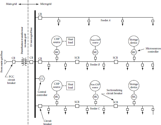
Germany had the leadership in wind turbine applications in the past. But, since then, the United States has taken over the leadership. (Figure 13.3 shows solar and wind applications in the city of Kassel in the state of Hessen in Germany. Figure 13.4 shows solar and wind turbine applications in the state of Rheinland-Pfalz in Germany. Figure 13.9 shows solar and wind turbine applications in the state of Rheinland-Pfalz in Germany.) The average commercial size of wind energy conversion system (WECS) was 300 kW until the mid-1990s. Today, there are wind turbines with a capacity of up to 6 MW that have been developed and installed. Since 1973, prices have dropped as performance has improved. Today, the cost of a wind turbine is below $2/W of installed capacity, and large wind farms with several hundred megawatt capacities are being developed over several months. For example, it is now quite common for wind power plants (wind farms) with collections of utility-scale turbines to be able to sell electricity for fewer than four cents per kWh. Early developments in California were basically in the form of wind farms, with tens of wind turbines, even up to 100 or more in some cases. The reasons for this development include the economies of scale that can be achieved by building wind farms, especially in construction and grid connection costs, and even possibly by getting quantity discounts from the turbine manufacturers. It is interesting to point out that the market introduction of wind energy is being done.
Solar and wind applications in the city of Kassel in the state of Hessen, Germany.
(SMA Solar Technology AG.)

Solar and wind turbine applications in the state of Rheinland-Pfalz in Germany.
(SMA Solar Technology AG.)
The European accessible onshore wind resource has been estimated at* 4800 TWh/year taking into account typical wind turbine efficiencies, with the European offshore resource in the region of 3000 TWh/year although this is very dependent on the assumed allowable distance from the shore. According to a recent report [1], by 2030 the EU could be generating 965 TWh from onshore and offshore wind, amounting to 22.6% of electricity requirements. The world onshore resource is approximately 53,000 TWh/year, considering siting constraints. Note the annual electricity demand for the United Kingdom and the United States are 350 and 3500 TWh, respectively.
13.9.1 Advantages and Disadvantages of Wind Energy Conversion Systems
The wind energy is the fastest growing energy source in the world due to many advantages that it offers. Continuous research efforts are being made even further to increase the use of wind energy.
13.9.2 Advantages of a Wind Energy Conversion System
- It is one of the lowest-cost renewable energy technologies that exist today.
- It is available as a domestic source of energy in many countries worldwide and not restricted to only few countries, as in case of oil.
- It is energized by naturally flowing wind; thus, it is a clean source of energy. It does not pollute the air and cause acid rain or greenhouse gases.
- It can also be built on farms or ranches and hence can provide the economy in rural areas using only a small fraction of the land. Thus, it still provides opportunity to the landowners to use their land. Also, it provides rent income to the landowners for the use of the land.
13.9.3 Disadvantages of a Wind Energy Conversion System
- The main challenge to using wind as a source of power is that the wind is intermittent and it does not always blow when electricity is needed. It cannot be stored; not all winds can be harnessed to meet the timing of electricity demands. At the present time, the use of energy storage in battery banks is not economical for large wind turbines.
- Despite the fact that the cost of wind power has come down substantially in the past 10 years, the technology requires a higher initial investment than the solutions using fossil fuels. Hence, depending on the wind profile at the site, the wind farm may or may not be as cost competitive as a fossil fuel-based power plant.
- It may have to compete with other uses for the land, and those alternative uses may be more highly valued than electricity generation.
- It is often that good sites are located in remote locations, far from cities where the electricity is needed. Thus, the cost of connecting remote wind farms to the supply grid* may be prohibitive.
- There may be some concerns over the noise generated by the rotor blades and esthetic problems that can be minimized through technological developments or by correctly siting wind plants [2].
13.9.4 Categories of Wind Turbines
Wind turbines turn the kinetic energy of the moving air into electric power or mechanical work. There are various WECSs. They can be classified as (1) horizontal-axis converters, (2) vertical-axis converters, and (3) upstream power stations.
Figure 13.5 shows three-blade wind energy converter that is the most common type of horizontal-axis converter for generating electricity worldwide. It shows the front and side views of a threeblade horizontal-axis wind energy converter. It has only a few rotor blades. Another conventional (older) type of horizontal-axis rotor is the multiblade wind converter. The horizontal-axis converters are of two types: with fast rotation or slow rotation.

The vertical axis converters are of two types: (1) Darrieus and (2) Savonius. The Darrieus converter has a vertical axis construction. They do not depend on the direction of the wind. But they have a low starting torque. Because of this, they need the help of a generator working as a motor or the help of Savonius rotor installed on top of the vertical axis.
The wind velocity increases substantially with height; as a result, the horizontal-axis wheels on towers are more economical. In the 1980s, a large number of Darrieus converters were installed in California, but a further expansion into a higher power range and their application worldwide has not happened. The Savonius rotor is used as a measurement device especially for wind velocity. However, it is used for power production for very small capacities under 100 W. The last technique mentioned previously is also known as “upstream power station” or thermal tower. It is a mix between a wind converter and a solar collector, poor efficiency, only about 1%.
Note that the terms “wind energy converters,” “windmills,” or “wind turbines” represent the same thing. The first one is the technical name of the system, whereas the other two are popularly used terms. Today, there are various types of wind energy converters that are in operation, as shown in Figure 13.6. Figure 10.7 shows eight different classes of wind turbines used in the Altamont pass in California.


Eight categories of wind turbines used in the Altamont Pass in California.
(From Orloff, S. and Flannery, A., Wind turbine effects on avian activity, habitat use, and mortality in altamont pass and Solano County wind resource areas: 1989-1991, California Energy Commission Report, No. P700-92,002; Stanon, C., Wind farm visual impact and its assessment, Wind Directions, BWEA, August 1995, pp. 8-9.)
Over the last 25 years, the size of the largest commercial wind turbines has increased from approximately 50 kW to 2 MW, with machines up to 6 MW under design. Figure 13.7 shows the main subsystems of a typical horizontal design. Figure 13.8 shows the main subsystems of a typical horizontal-axis wind turbine. These include the rotor, including the blades and supporting hub; the drive train, which includes the rotating parts of the wind turbine (except the rotor), including shafts gearbox, coupling, a mechanical brake, and the generator; the nacelle and main frame, including wind turbine housing, bedplate, and the yaw system; the tower and the foundation; and the machine controls, the switchgear, transformers, and possibly electronic power converters.

There are a number of options in wind machine design and construction. These options include the number of blades (normally two or three); the blade material, construction method, and profile; the rotor orientation, downward or upward of tower; hub design, rigid, teetering, or hinged; fixed or variable rotor speed; orientation by self-aligning action (free yaw) or direct control (active yaw); power control via aerodynamic control (stall control) or variable pitch blades (pitch control); synchronous or induction generator; and gearbox or direct-drive generator.
Almost all wind turbines use either induction or synchronous generators. Both of these designs entail a constant or nonconstant rotational speed of the generator when the generator is directly connected to a utility network. The majority of wind turbines installed in grid-connected applications use induction generators. An induction generator operates within a narrow range of speeds slightly higher than a narrow range of speeds slightly higher than its synchronous speed. The main advantage of induction generators is that they are rugged, inexpensive, and easy to connect to an electric network. An induction generator is much simpler to connect to the grid than a synchronous generator.
The nacelle of horizontal-axis turbine contains a bedplate on which the components are mounted. There is a main shaft with main bearings, a generator, and a yaw motor that turns the nacelle and rotor into the wind. The nacelle cover protects the contents from the weather. Nacelle and yaw system include the wind turbine housing, the machine bedplate or main frame, and the yaw orientation system. The main frame provides for the mounting and proper alignment of the drive train components.
A yaw orientation system is needed to keep the rotor shaft properly aligned with the wind. The main component is a large bearing that connects the main frame to the tower. An active yaw drive, generally used with an upwind turbine, has one or more yaw motors, each of which drives a pinion gear against a bull gear attached to the yaw bearing. This mechanism is controlled by an automatic yaw control system with its wind direction sensor usually mounted on the nacelle of the wind turbine. Sometimes yaw brakes are used with this type of design to hold the nacelle of the wind turbine. Free yaw systems are normally used on downwind wind machines. They can self-align with the wind. The control system of a wind turbine includes sensors, controllers, power amplifiers, and actuators.
13.9.5 Types of Generators Used in Wind Turbines
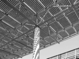
There are three types of electrical machines that can convert mechanical power into electric power, which are the direct current (dc) generator, the synchronous alternator, and the induction generator. In the past, the shunt-wound dc generators were commonly used in small battery charging wind turbines. In these generators, the field is on the stator and the armature is on the rotor. A commutator on the rotor rectifies the generated power to dc.
By regulating the speed of the generator (i.e., wind turbine) and/or its field, the dc voltage can be maintained with a specified range. Speed regulation is usually performed by changing the pitch of the propeller blades. If the dc voltage is sensed, the field strength can be varied according to the control of the generated voltage. As illustrated in Figure 13.9a, a transmission that increases the rotating blade speed to that required for the generator has to be included.
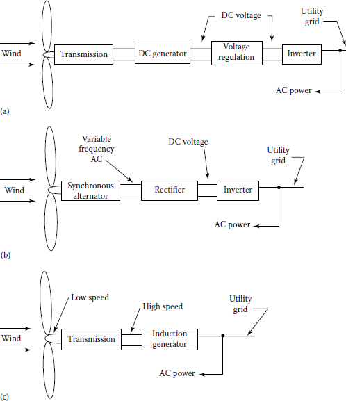
Block diagram of a WECS: (a) using a dc generator, (b) using a synchronous alternator, and (c) using induction generator.
The field current and thus magnetic field increase with operating speed. The armature voltage and electrical torque also increases with speed. The actual speed of the turbine is determined by a balance between the torque from the turbine rotor and the electrical torque. Since the wind speed is variable over a wide range, some regulation method must be used, as shown in Figure 13.10.

A wind machine typically rotates at a speed in the range of 50–100 rpm (i.e., about 5–10 rad/s). Depending on the generator, this has to be geared up to 1000–2000 rpm (i.e., about 100–200 rad/s). The net efficiency of the energy conversion system is a function of the efficiency of the blades, transmission, generator, regulating circuitry, and inverter. However, dc generators of this type are seldom used today because of high costs and maintenance requirements (due to the commutators).
Permanent magnet generators are used in most small wind turbine generators, up to at least 10 kW. Here, permanent magnets provide the magnetic field. Hence, there is no need for field windings, or supply current to the field, nor there is any need for commutators, slip rings, or brushes. The permanent magnet generator is quite rugged since the machine construction is so simple. Their operating principles are similar to that of synchronous machines, with the exception that they are run asynchronously. In other words, they are not generally connected directly to the alternating current (ac) network. The power produced by the generator is initially variable voltage and frequency ac. This ac variable voltage is often rectified immediately to dc. The resultant dc power then either directed to dc loads or battery storage, or else it is inverted to ac with a fixed frequency and voltage.
Synchronous machines operate at constant speed, with only the power angle changing as the torque varies. Synchronous machines hence have a very “stiff” response to fluctuating conditions. An alternator produces an ac voltage whose frequency is proportional to shaft speed. Even with speed regulation, there will still be enough of a variation in frequency and phase to prevent connection of the alternator directly to the utility grid.
Therefore, the alternator is permitted to turn at different speeds, producing a variable-frequency output. The alternator output is then rectified, converting it to dc, as shown in Figure 13.9b. The magnitude will be constant since the alternator field is constant. It is usually a permanent magnet alternator. The dc is now fed to a synchronous inverter, whose line frequency output can be connected directly to the utility grid. Here, the need for transmission is eliminated and the alternator can be connected directly to the wind wheel.
The induction generator is well suited for a wind energy system provided that utility power is available. But in order for the induction machine to operate as a generator, a separate source of reactive power is necessary to excite the machine. Also, the induction generator must be driven slightly faster than synchronous speed. However, it is not necessary for the speed to be constant, merely to maintain a negative slip. Rated power and peak efficiency are generally achieved at about -3% slip, not the speed of its rotor.
The only components required for this WECS are a transmission to gear the speed of the blades up to that necessary for the negative slip and the induction generator, as represented in Figure 12.9c. However, in the event of a loss of utility, power automatically disables the WECS since the field excitation no longer exists. The net system efficiency depends on the efficiency of the blades, transmission, and generator. But some means of speed regulation is required to maintain the required slip.
Note that when a constant torque is applied to the rotor of an induction machine, it will operate at a constant slip. If the applied torque is varying, then the speed of the rotor will vary as well. This relationship can be described by the following equation:
Jdωrdt=Qe−Qr(13.3)
where
- J is the moment of inertia of the generator rotor
- ωr is the angular speed of the generator rotor (rad/s)
- Qe is the applied electrical torque
- Qr is the torque applied to the generator rotor.
Induction machines are somewhat “softer” in their dynamic response to changing conditions than are synchronous machines. This is due to the fact that induction machines undergo a small but significant speed change (slip) as the torque in or out changes.
Induction machines are designed to operate at a specific operating point. This operating point is usually defined as the rated power at a specific frequency and voltage. However, in wind turbine applications, there may be a number of cases when the machine may run at off-design conditions. These conditions include starting, operation below rated power, variable-speed operation, and operation in the presence of harmonics. The operation below rated power, but at rated frequency and voltage, is a common occurrence. It normally presents few problems. But efficiency and power factor are generally both lower under such conditions.
In general, there are a number of benefits of running a wind turbine rotor at variable speed. A wind turbine with an induction generator can be run at variable speed if the electronic power converter of approximate design is included in the system between the generator and the rest of the electric network.
Such converters operate by changing the frequency of the ac supply at the terminals of the generator. These converters also have to vary the applied voltage. It is due to the fact that an induction machine performs best when the ratio between frequency and voltage, that is, “volts to hertz ratio,” of the supply is constant or almost constant. When that ratio departs from the design value, a number of problems can take place. For example, currents may be higher, causing higher losses and possible damage to the generator windings.
Finally, operation in the presence of harmonics can take place, if there is a power electronic converter of significant size on the system to which the induction machine is connected. Also, harmonics may cause bearing and electrical insulation damage and may interfere with electrical control or data signal as well.
13.9.6 Wind Turbine Operating Systems
Depending on controllability, wind turbine operating systems are categorized as (1) constant-speed wind turbines and (2) variable-speed wind turbines.
13.9.6.1 Constant-Speed Wind Turbines
They operate at almost constant speed as predetermined by the generator design of gearbox ratio. The control schemes are always aimed at maximizing either energy capture by controlling the rotor torque or the power output at high winds by regulating the pitch angle. Based on the control strategy, constant-speed wind turbines are again subdivided into (1) stall-regulated turbines and (2) pitch-regulated turbines.
Constant-speed stall-regulated turbines have no options for any control input. Its turbine blades are designed with a fixed pitch to operate near the original tip speed ratio (TSR) for a given wind speed. When wind speed increases, it causes a reduced rotor efficiency and limitation of the power output. The same result can be achieved by operating the wind turbine at two distinct constant operating speeds by either changing the number of poles of the induction generator or changing the gear ratio.
The stall regulation has the advantage of simplicity. But it has the disadvantage of not being able to capture wind energy in an efficient manner at wind speeds other than the design speed. They use pitch regulation for staring up. They have the following advantages:
- They have a simple, robust construction and electrically efficient design.
- They are highly reliable since they have fewer parts.
- No current harmonics are produced since there is no frequency conversion.
- They have a lower capital cost in comparison to variable-speed wind turbines.
On the other hand, their disadvantages include the following:
- They are aerodynamically less efficient.
- They are prone to mechanical stress and are noisier.
13.9.6.2 Variable-Speed Wind Turbines
Figure 13.10 shows a typical variable-speed pitch-regulated wind turbine system. It has two methods for controlling the turbine operation in terms of speed changes and blade pitch changes. The control strategies that are usually used are power optimization strategy and power limitation strategy.
Power optimization strategy is used when the wind speed is below the rated value. It optimizes the energy capture by keeping the speed constant based on the optimum TSR. However, if speed is changed because of load variation, the generator may be overloaded for wind speeds above nominal value. In order to prevent this, methods like generator torque control are employed to control the speed.
On the other hand, the power limitation strategy is used for wind speeds above the rated value by changing the blade pitch to reduce the aerodynamic efficiency. The advantages of the variablespeed wind turbine systems include the following:
- They are subjected to less mechanical stress and they have high energy capture capacity.
- They are aerodynamically efficient and have low transient torque.
- They require no mechanical damping systems since the electric system can effectively provide the damping.
- They do not suffer from synchronization problems or voltage sags because they have stiff electrical controls.
The disadvantages of the variable-speed wind turbine systems include the following:
- They are more expensive.
- They may require complex control strategies.
- They have lower electrical efficiency.
In general, in order to indicate how much wind power there is in a country, the total installed capacity is used as a measure. Every wind turbine has a rated power (maximum power) that can vary from a few hundred watts to 5000 kW (5 MW). The number of turbines does not give any information on how much of wind power they can produce.
How much wind a wind turbine can produce depends not only on its rated power but also on the wind conditions. In order to get an indication of how much a certain amount of installed (rated) power will produce per year, use the following rule of thumb: “1 MW wind power produces 2 GWh per year on land and 3 GWh per year offshore.”
13.9.7 Meteorology of Wind
The fundamental driving force of air is a difference in air pressure between two regions. This air pressure is governed by various physical laws. One of them is known as Boyle’s law. It states that the product of pressure and volume of a gas at a constant temperature must be constant. Thus,
p1ν1=p2ν2(13.4)
Another law is Charles’ law. It states that for a constant pressure, the volume of a gas varies directly with absolute temperature. Hence,
ν1T1=ν2T2(13.5)
Therefore, at -273.15°C or 0 K, the volume of a gas becomes zero.
The laws of Charles and Boyle can be combined into the ideal gas law. That is,
pν=nRT(13.6)
where
- p is the pressure in pascal (N/m2)
- ν is the volume of gas in cubic meters
- n is the number of kilomoles of gas
- R is the universal gas constant
- T is the temperature in kelvin
At standstill conditions (i.e., 0°C and 1 atm), 1 kmol of gas occupies 22.414 m3 and the universal gas constant is 8314.5 J/(kmol · K), where J represents a joule or newton meter of energy. The pressure of 1 atm at 0°C is then
p=[8314.5 J/(kmol⋅K)](273.15 K)22.414 m3=101,325 Pa=101.325 kPa(13.7)
The mass of 1 kmol of dry air is 28.97 kg. For all ordinary purposes, dry air behaves like an ideal gas.
The density ρ of a gas is the mass m of 1 kmol divided by the volume v of that kilomole:
ρ=mv(13.8)
The volume of 1 kmol varies with pressure and temperature as defined by Equation 13.6. By inserting Equation 13.8 into Equation 13.9, the density can be expressed by the following equation:
ρ=mpRT=3.484pRTkg/m3(13.9)
where
- p is in kilopascal (kPa)
- T is in kelvin (K)
This expression yields a density for dry air at standard conditions of 1.293 kg/m3.
The common unit of pressure used in the past for meteorological work has been the bar (i.e., 100 kPa) and the millibar (100 Pa). A standard atmosphere is 1.01325 bar or 1013.25 millibar.
Atmospheric pressure has also been given by the height of mercury in an evacuated tube. This height is 29.92 in. or 760 mm of mercury for a standard atmosphere. Also note that the chemist uses 0°C as standard temperature, whereas engineers have often used 68°F (20°C) or 77°F (25°C) as standard temperature. Therefore, here standard conditions are always defined to be 0°C and 101.3 kPa pressure.
Most wind-speed measurements are made about 10 m above the ground. Typically, small wind turbines are mounted 20–30 m above ground level, while the propeller tip may read a height of more than 100 m on the large turbines. Thus, an estimate of wind-speed variation with height is needed. Here, let us examine a property that is known as atmospheric stability in the atmosphere.
Pressure decreases quickly with height at low attitudes, where density is high, and slowly at high altitudes where density is low. At sea level and a temperature of 273 K, the average pressure is 101.3 kPa. A pressure of half this value is reached at about 5500 m.
A temperature decrease of 30°C will often be related to a pressure increase of 2–3 kPa. The atmospheric pressure tends to be a little higher in the early morning than in the middle of the afternoon. Winter pressure tends to be higher than summer pressures.
The power output of a wind turbine is proportional to air density, which in turn is proportional to air pressure. Hence, a wind speed produces loss power from a given wind turbine at higher elevations, due to the fact that the air pressure is less. A wind turbine located at an elevation of 1000 m above sea level will produce only about 90% of the power it would produce at sea level, for the same wind speed and air temperature.
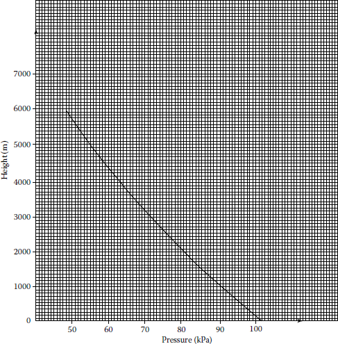
However, there are many good wind sites in the United States at elevations above 1000 m. The air density at a proposed wind turbine site is estimated by determining the average pressure at that elevation from Figure 13.11 and then using Equation 12.7 to find density. The ambient temperature must be used in the equation.
Example 13.1
Consider a wind turbine that is rated at 100 kW in a 10 m/s wind speed in air at standard conditions. If power output is directly proportional to air density, determine the power output of the wind turbine in a 10 m/s wind speed at a temperature of 20°C at a site that has the elevation of
- 1000 m above sea level
- 2000 m above sea level
Solution
- From Figure 13.11, the average pressure at the 1000 m elevation is 90 kPa, and from Equation 13.9, the density at 20°C = 293 K is
ρ=3.484pT=3.484(90)293=1.070
Thus, the power output at the conditions is just the ratio of this density to the density at standard conditions times the power at standard conditions:
Pnew=Pold(ρnewρold)=100(1.0701.293)=82.75 kW
- From Figure 13.11, the average pressure of the 2000 m elevation is 80 kPa, and since the temperature is still 20°C = 293 K, the density is
ρ=3.484pT=3.484(80)293=0.951
Hence, the power at the 2000 m elevation is
Pnew=Pold(ρnewρold)=100(0.9511.293)=73.55 kW
Note that the power output has dropped from 100 to 82.75 kW at the same wind speed at the 1000 m elevation and to 73.55 kW at the 2000 m elevation due to the fact that there are lesser air densities at the higher elevations.
13.9.7.1 Power in the Wind
The wind speed is always fluctuating, and thus, the energy content of the wind is always changing. The variation depends on the weather and on local surface conditions and obstacles to the wind flow. Power output from a wind turbine will vary as the wind varies, even though the most rapid variations will to some extent be compensated for by the inertia of the wind turbine rotor.
It is common knowledge around the globe that it is windier during the daytime than at night. This variation is mostly as a result of temperature differences that tend to be larger during the day than at night.
Furthermore, the wind is also more turbulent and tends to change direction more frequently during the day than at night. Therefore, forecasting the amount of electric energy that can be harnessed over a period of time is extremely difficult.
Consider the wind turbine shown in Figure 13.5 and assume that the wind blows perpendicularly through a circular cross-sectional area. A wind generator will capture only the wind power caught by the given swept area A that can be expressed in watts in SI system as
P=12ρaAv3(13.10)
where
- ρa is the mass density of air (and is relatively constant)
- A is the circular cross-sectional area in m2 (i.e., A = πr2)
- r is the radius of the circular cross-sectional area in m
- ν is the wind velocity in m/s
For the average mass density of air, ρa = 1.24 kg/m3 or in British system in ft.lb/s as
P=12ρaAv3(746550)(13.11a)
or
P=0.678 ρaAv3(13.11b)
where
= 0.0024 lb · s2/ft4
A is in ft2
ν is in ft/s
Note that since the wind speed is usually given in miles per hour (mph), it needs to be converted into ft/s by using
vft/s=1.47vmph(13.12)
The following equation gives an improved version of the previous equation to determine the power in the wind in watts,
P=12ρaAv3Cp(13.13)
where Cp is the turbine power coefficient, which represents the power conversion efficiency of wind turbine. It gives a measure of the amount of power extracted by the turbine rotor. Its value varies with rotor design and the TSR.
TSR is the relative speed of the rotor and the wind and has a maximum practical value of about 0.4. The ratio of the tip speed of the machine turbine blades to wind speed is found from
λ=r×Ωv(13.14)
where
- r is the radius of the circular cross-sectional area (i.e., turbine radius)
- Ω is the tip speed of the machine turbine blades
- ν is the wind speed
Figure 13.12 shows various tip speed diagrams for various types of wind energy converters.

TSR diagrams for various types of wind energy converters.
(The power coefficient gives a measure of how large a share of the wind’s power a turbine can utilize. The theoretical maximum of the value is 16/27 = 0.5926. The diagram shows the relation between TSR and power coefficient for different types of wind turbines: (a) windmill, (b) modern turbine with three blades, (c) vertical-axis Darrieus turbine, and (d) modern turbine with two blades.)
Here, the TSR (λ) is the relation between the speed νtip and undisturbed wind speed ν0 and is signified by λ. Thus,
λ=tangential velocity of blade tipwind speed(13.15a)
or
λ=vtipv0(13.15b)
Previously, the power present in a wind for a given velocity and swept area was given by Equation 13.10 or 13.11b. However, all of this power cannot be collected by wind turbine. The theoretical maximum fraction of available wind power that can be collected by a wind turbine is given by the Betz coefficient.
The energy in the wind is kinetic energy. In order to capture this energy, the blades of a wind turbine have to slow down as it passes through them. Hence, after the wind has passed through the wind turbine, its velocity (thus, its kinetic energy) is less than it originally had. Here, the energy it lost has been converted to the kinetic energy of the rotating blades. If after passing through the blades, the wind speed has decreased to one-third of its initial value, the blades will have theoretically captured a maximum fraction of the available wind energy. This maximum energy is given by
Beta coefficient=0.5926
This means that the actual power input for a wind turbine will be (at best) 59% of the power provided by Equation 13.10 or 13.11b. The actual blade efficiency is somewhat less than the Betz coefficient. It is a function of a quantity called the TSR λ, as explained in Equation 13.14. The power coefficient Cp gives a measure of how large portion of the wind’s power a turbine can utilize. The theoretical maximum value of Cp is 16/27 = 0.5926. The curves in Figure 13.12 show the relation between TSR and power coefficient for different types of wind turbines: (1) windmill, (2) modern turbine with three blades, (3) vertical-axis Darrieus turbines, and (4) modern turbine with two blades. Note that the turbine power coefficient Cp is maximum at the λ optimal. Also note that the wind turbine system uses induction generators that are independent of torque variation while speed varies between 1% and 2%. In general, there is a great amount of power in the wind. However, this mechanical power when it is converted to electric power is reduced substantially. A typical WECS has an efficiency of 20%–30%.
Example 13.2
Determine the amount of power that is present in a 10 m/s wind striking a windmill whose blades have a radius of 5 m.
Solution
The area swept by the blades of the wind turbine is
A=πr2=π(5 m)2≅78.54 m2
Thus, the power that is present in the wind is
If the turbine power coefficient (Cp) is 0.20, then the amount that will be converted to usable electric power is
which is considerably lesser than the power that is preset in the wind.
13.9.8 Effects of a Wind Force
In any WECS, the support of the tower on which the wind generator is mounted must be considered; when a wind blows on a wind turbine, it applies a force on the blades. This wind force applied to the blades is determined in SI or British system from
Additionally, the wind force applied on the tower (Ft) carrying the wind turbine has to be considered. The resultant effect of these forces is to develop a moment about the tower base in the clockwise direction. This overturning moment is a function of the wind speed, size of the blades, and the height of the wind turbine.
Because of this, large wind turbines mounted on high towers must be properly supported. Also, many wind turbines have an automatic high-wind shutdown feature. This feature automatically turns the blades so that they become parallel to the wind and it can escape any damage to the WECS system.
13.9.9 Impact of Tower Height on Wind Power
As general rule, a taller tower is expected to result in higher-speed winds to the wind turbine. However, surface winds can also be affected by the irregularities or roughness of the earth’s surface or by the existing forest and/or buildings in the vicinity. The relationship between the wind speed and the height of the wind turbine can be expressed as
where
- ν is the wind speed at height H
- ν0 is the reference (or known) wind speed at reference height of H0
- α is the roughness (friction) sufficient
In Europe, the relationship in Equation 13.17 is modified as
There are many factors that affect wind, for example, elevation, contour of the ground in the surrounding areas, tall buildings, and trees. The average wind speed will be probably different at different tower heights. In the event that the average wind speed at different heights is the same, the location with shorter height should be considered since such application results in less expensive tower.
Furthermore, at a higher elevation having greater wind, it is possible to use a smaller wind turbine with shorter blade diameter, rather than using a large turbine with larger blade diameter at a lower elevation for obtaining the same amount of power.
The value of the exponent α in Equation 13.17 depends on the roughness of the terrain given in Table 13.2
Roughness Coefficient for Various Class Types of Terrain
Roughness Class |
Terrain Description |
Roughness Coefficient (α) |
|---|---|---|
Class 0 |
(Open water) |
α = 0.1 |
Class 1 |
(Open plain) |
α = 0.15 |
Class 2 |
(Countryside with farms) |
α = 0.2 |
Class 3 |
(Villages and low forest) |
α = 0.3 |
Example 13.3
If the average wind speeds on an open plain (roughness class 1) is known to be 6 m/s at 10 m height, determine the wind speed at 50 m height.
Solution
From Table 13.2, α = 0.15 and using Equation 13.15,
or
Thus, at 50 m height,
Example 13.4
Assume that the average wind speed at a point A is 6 m/s, while at point B 7 m/s. In order to capture 2 kW, determine the blade diameter d for a wind turbine operating
- At point A
- At point B
Solution
- Using Equation 13.12, the given wind speed needs to be converted to ft/s as
and
From Equation 13.11b, at point A,
Since
then
- At point B,
Thus,
Therefore, a smaller (cheaper) wind turbine could be employed at point A and provide the same power as a larger wind turbine at point B.
13.9.10 Wind Measurements
Wind measurement equipment usually consists of an anemometer, which measures wind speed, and a wind vane, which measures wind direction. In most countries, a national meteorological institute has measured and collected data on the winds since the nineteenth century. They register wind speed, wind direction, temperature, and other kinds of meteorological data several times a day (every 4 h, day and night) all year around. These data are reported daily to a central institution.
Nowadays, wind data are registered automatically. These observations make up the basis for the wind statistics that are used to describe wind climate in different regions and to create so-called wind atlas data that are used to calculate how much wind turbines can be expected to produce at different sites.
However, in the past, weather observers read the anemometer every 4 h, day and night. They observed the anemometer for a couple of minutes and recorded the average wind speed for that period. However, wind-speed data are affected by the anemometer height, the human factor in reading the wind speed, and the quality and maintenance of the anemometer.
A typical wind-cup anemometer works with a diametric flow of air. As the wind blows, the anemometer rotates at a speed proportional to the wind speed. Typically, a permanent magnet dc generator is connected to the rotating shaft. A voltage is thus produced that is proportional to the wind speed at every instant of time. The second instrument that is required is a wind data compilator. It is an electronic instrument that is connected to the anemometer and records the wind speed continuously.
Example 13.5
Consider a wind turbine that has blades with 8 ft radius. At its location where it is mounted, data were taken and it was discovered that the wind speed was 3 mph for 3 h and 12 mph for another 3 h time period. Determine the amount of energy that can be intercepted by the wind turbine.
Solution
The energy needs to be determined independently for each 3 h period.
During the first 3 h time period,
the average wind speed is
By using Equation 13.11b,
where
During the second 3 h time period,
the average wind speed is
By using Equation 13.11b,
Therefore, the total energy generated during the total period is
Hence, total energy is
13.9.11 Characteristics of a Wind Generator
The most important characteristic of a wind generator is its power curve. Normally, it is a graph provided by the manufacturer of a particular wind turbine. It shows the approximate power output as a function of wind speed. Figure 13.13 shows a typical power curve for a wind turbine rated 3 kW/25 mph. The power curve of a wind generator provides important information. In addition, to provide information for the obtainable power output at any given wind speed, it provides information about the cut-in speed, the rated power, the rated speed, and the shutdown speed.

Here, the minimum wind speed required to start the blades turning and producing a useful output is defined as the cut-in speed. The maximum power output that the wind turbine will produce is called the rated power.
The minimum wind speed needed for the wind turbine to produce rated power is known as the rated speed. The shutdown speed is also called the furling speed. It is the maximum operational speed of the wind turbine. Beyond this speed, in order to prevent damage to the system from high winds, the blades are either folded back or turned to a high-pitch position.
Example 13.6
Consider the wind turbine whose power curve of its generator is shown in Figure 13.13. It is rated 3 kW/25 mph, as indicated in the figure. Assume that during an 8 h period, the wind had the following average speeds: 6 mph for 2 h duration, 10 mph for 3 h duration, 15 mph for 2 h duration, and 20 mph for 1 h duration. Determine the resultant electric output for the 8 h period.
Solution
The energy is calculated for each of the four wind speeds and time intervals:
At 6 mph, it is below the cut-in speed in Figure 13.13; thus, the output is zero.
At 10 mph, the output from the curve is 0.35 kW:
At 15 mph, the output from the curve is 0.85 kW:
At 20 mph, the output from the curve is 1.65 kW:
Thus, the total energy for 8 h duration is
13.9.12 Efficiency and Performance
How much energy a wind turbine can produce is a function of a number of factors: the rotor swept area, the hub height, and how efficiently the wind turbine can convert the kinetic energy of the wind. Also the additional factors include the mean wind speed and the frequency distribution at the site where the wind turbine is installed.
The power of the wind that is available to a turbine is proportional to the rotor swept area A and the cube of the wind speed v. Over the years, the rotor swept area of wind turbines has increased steadily and thus so has the rated power of the wind turbines, as given in Table 13.3. Note that the production figures given in the table are based on a site with average wind resources. It appears that since the 1980s, the power of wind turbines has doubled every 4–5 years on the average.
Development of Wind Turbine Size, 1980–2005
Year |
1980 |
1985 |
1990 |
1995 |
2000 |
2005 |
|---|---|---|---|---|---|---|
Power (kW) |
50 |
100 |
250 |
600 |
1000 |
2500 |
Diameter (m) |
15 |
20 |
30 |
40 |
55 |
80 |
Swept area (m2) |
177 |
314 |
706 |
1256 |
2375 |
5024 |
Production (MWh/year) |
90 |
150 |
450 |
1200 |
2000 |
5000 |
Source: From Wizelius, T., Developing Wind Power Projects: Theory and Practice, Earthscan, London, U.K., 2007.
Example 13.7
Assume that a wind generator whose power curve is shown in Figure 13.13 has a blade diameter of 16 ft. If its power output is at 120 V at 60 Hz, determine the net efficiency of this WECS at a wind speed of 20 mph.
Solution
First, it is necessary to convert the wind speed from mph to ft/s by using Equation 13.12:
The input power is found from Equation 13.11b as
From Figure 13.13, the output power at 20 mph is
Thus, the efficiency of the system is
Example 13.8
Assuming that the wind turbine with three blades in Example 13.7 is rotating at 100 rpm, find the blade efficiency at a wind speed of 20 mph.
Solution
The circumference that the blade tip traces out is
The blade tip speed is
From Equation 13.15b,
From Figure 13.12, for λ = 2.85, the blade efficiency is about 13%. Note that the share of power in the wind that can be utilized by the rotor is called the power coefficient, Cp.
Example 13.9
Assume that a WECS shown in Figure 13.9c uses a three-phase six-pole induction machine. The line frequency is 60 Hz and the average wind speed is 12 mph. The blades have a 30 mph diameter and peak efficiency when the TSR is 8.3. If the generator efficiency is a maximum at a negative lip of 3.3%, determine the transmission gear ratio for the peak system efficiency.
Solution
At first, the speeds required for the blades and generator have to be found. Then the transmission will be selected to match the two speeds. The required generator speed is
From Equation 13.12, the average wind speed is
From Equation 13.15b, the blade tip speed is
The circumference traced out by the blade tip is
Hence, the blade tip speed must be
Converting this to rpm,
Therefore, the transmission must gear up from 93.21 rpm to 1239.6 rpm. Hence, the required gear ratio is
13.9.13 Efficiency of a Wind Turbine
In order to calculate the efficiency of a wind turbine, the efficiency of its components has to be calculated at first.
13.9.13.1 Generator Efficiency
A wind turbine can never utilize all the power in the wind. The amount of power that can be utilized by a wind turbine is given by the power coefficient Cp. It is known that (based on Bets’ law) the maximum value of this coefficient is 0.59. It varies with the wind speed. For most wind turbines, the maximum value varies between 0.45 and 0.50 at a wind speed of 8–10 m/s for most wind turbines.
In order to convert the power in the wind from the revolving rotor to electric power, it is passed through a gearbox and a generator or, for direct-drive turbines, through a generator and an inverter. In this conversion process, some power will be lost. Also, the efficiency of the individual components will vary with the wind speed.
It is known that a generator is most efficient when it is running at its nominal power. On a wind turbine, most of the time the generator is operating on partial load, that is, it runs on lower power when the wind speed is lower than the nominal wind speed. As a result, the standard generator efficiency will then be reduced, as given in Table 13.4.
There is also a relationship between the physical size of a generator and efficiency. That is, efficiency increases with the size of the generator, since losses to heat are reduced, as given in Table 13.5.
Relationship between Size and Efficiency
Nominal Power (kW) |
5 |
50 |
500 |
1000 |
|---|---|---|---|---|
Efficiency |
0.84 |
0.89 |
0.94 |
0.95 |
For example, a 1 MW wind turbine running at 20% of its nominal power (200 kW) has an efficiency of 0.95 × 0.90 = 85%. Note that the relationship between efficiency, size, and partial load can also differ between different models and manufacturers.
13.9.13.2 Gearbox
Typically on a large modern wind turbine, the rotor has a rotational speed of 20–30 rpm, while the generator will need to rotate at 1520 rpm. In order to increase the speed, a gearbox is used. If the turbine rotor runs at 30 rpm, a gear change of 30:1520 = 1:50.7 is required. That is, 1 rev of the main shaft has to be increased to 50.7 rev on the secondary shaft that is connected to the generator.
Generally, a gearbox has several steps; thus, the rotational speed is increased stepwise. Losses can be estimated at 1% per step. In wind turbines, three-step gearboxes are usually used and the efficiency of the gearbox will then be about 97%.
However, wind turbines with a direct-drive generators and variable speed do not need any gearbox. Instead the frequency and voltage of the electric current will vary with the rotational speed. Thus, the current has to be rectified to dc and then converted by an inverter to ac with the same frequency and voltage as the grid. The efficiency of such an inverter is also about 97%.
13.9.13.3 Overall Efficiency
In summary, the overall efficiency ηtotal l of a wind turbine is the product of the turbine rotor’s power coefficient Cp and the efficiency of the gearbox (or inverter) and generator
Often Cp is set to 0.59 and μrotor (or μr) is used to show how large a share of the theoretically available power the rotor can utilize. For example, if the power coefficient Cp = 0.49, the rotor turbine charges is then
The efficiency of a wind turbine changes with the wind speed. When the wind speed is below the nominal wind speed, the efficiency of the generator will decrease, and if the turbine has a fixed rotational speed, the TSR will change, that is, the ever smaller share of the power in the wind will be utilized and Cp will decrease successfully. Since the wind turbines are used to convert wind power to electric power, and thus another coefficient is used, Cp, which indicates the turbine rotor’s power coefficient.
13.9.13.4 Other Factors to Define the Efficiency
In order to estimate efficiency, the following factors are also often used:
Availability is the technical reliability of a wind turbine. If the wind turbine is out of operation due to faults or scheduled service and maintenance for 5 days a year, the technical availability is 98.6%. (A year is normally taken as 360 days for such calculations.)
It means that the turbine could produce power for 98.6% of the time, if there was always enough wind to make the run. The technical lifetime for a turbine is estimated at 20–25 years. However, its economic lifetime can be shorter due to increased maintenance costs as the turbine gets old.
There is another factor that is used to indicate the capacity factor. It is called annual load factor and defined as
Here, the significance of load duration is that it expresses that number of hours for which the wind turbine can be considered to be virtually operating at its rated capacity in 1 year.
In general, in order to indicate how much wind power there is in a country, the total installed capacity is used as a measure. Every wind turbine has a rated power (maximum power) that can vary from a few hundred watts to 5000 kW (5 MW). The number of turbines does not give any information on how much of wind power they can produce.
How much wind a wind turbine can produce depends not only on its rated power but also on the wind conditions. In order to get an indication of how much a certain amount of installed (rated) power will produce per year, use the following rule of thumb: “1 MW wind power produces 2 GWh per year on land and 3 GWh per year offshore.”
Example 13.10
Consider a 4 MW wind turbine that is under maintenance for 400 h in 1 year; out of 8760 h of 1 year. If it actually produced 8000 MWh due to fluctuations in wind availability, determine the following:
- The availability factor of the wind turbine
- The capacity factor of the wind turbine
- The annual load duration of the wind turbine
Solution
- The availability factor of the wind turbine is
- The capacity factor of the wind turbine is
- The annual load duration for the wind turbine is
However, the capacity factor of 0.4566 (or 45.66%) does not mean that the wind turbine is only running less than half of the time. Rather, a wind turbine at a typical location would normally run for about 65%–90% of the time. But, much of the tie, it will be generating at less than full capacity, causing its capacity factor lower.
13.9.14 Grid Connection
The term grid is often used loosely to describe the totality of the network. Specifically, grid connected means connected to any part of the network. The term national grid usually means the EHV transmission network.
Integration particularly means the physical connection of the generator to the network with due regard to the secure and safe operation of the system and the control of the generator so that the energy resource is utilized optimally. The integration of generator power from wind turbine (or any other renewable energy sources) is basically similar to that of fossil fuel-powered generator and is based on the same principles. However, renewable energy sources are often variable and geographically dispersed. The connection point is referred to as the PCC.
Wind power can be classified as small and non-grid connected, small and grid connected, large and non-grid connected, and large and grid connected. The small and non-grid-connected type of wind turbine can be used in a location that is not served by a utility. It can be improved by adding batteries to level out supply and demand. The cost will be high about $0.50/kWh. The small and grid-connected wind turbine is usually not economically feasible.
The economic feasibility can be improved, if the local utility is willing to provide an arrangement that is called net metering. In such system, the meter runs backward when the turbine is generating more than the owner is consuming at the moment. The owner pays a monthly charge for the wires to his home.
In general, utilities want to buy at wholesale and sell at retail. It is often that the owner might pay $0.08–$0.15/kWh and get paid $0.02/kWh for the wind-generated electricity that is far from enough to economically justify a wind turbine.
Wind speed is the main factor in determining electricity cost, in terms of influencing the energy yield, and approximately, at the locations with wind speeds of 8 m/s, it will yield electricity at onethird of the cost for a 5 m/s site. Wind speeds of approximately 5 m/s can typically be found at the locations away from the coastal areas. However, wind energy developers usually intend to find higher wind speeds. Levels at about 7 m/s can be found in many coastal regions.
The large and non-grid-connected wind turbines are installed on islands or in some native villages where it is virtually impossible to connect to a large grid. In such places, one or more wind turbines can be installed in parallel with the diesel generators so that the wind turbines can act as fuel savers when the wind is blowing. This system can operate easily. In general, the justification for having the small or the large wind turbines must be based on whether or not it will result in a lower net cost to society, including the environmental benefits of wind generation. Today, wind turbines with ratings near 1 MW or more are now common.
However, this is still small compared to the needs of a utility, so clusters of turbines are placed together to form wind farms or wind plants with total ratings of 10–100 MW, or even more. Presently, Southern California Edison (SCE) Company is working on Tehachapi Renewable Transmission Project (TRTP) of 500 kV. The purpose of the proposed TRTP project is to provide the electrical facilities necessary to integrate levels of new wind generation in excess of 700 MW and up to approximately 4500 MW in the future in the Tehachapi Wind Resource Area (TWRA) in Southern California.
The voltage level of large wind turbines, in general, is 600 V, so-called industrial voltage. Therefore, they can be connected to a factory without a transformer. Smaller wind turbines, up to 300 kW, which were common in the near past, have a voltage of 480 V and can be connected directly via a feeder cable to a farm or a house. However, usually wind turbines are connected to the power grid through a transformer that increases the voltage level from 480 or 600 V to the higher voltage, normally 10 or 20 kV, in the distribution grid. A suitable transformer is installed on the ground next to the tower for smaller- and medium-sized wind turbines. But in large wind turbines, the transformer is often a component of the turbine itself.
In modern wind turbines, the power that is supplied into the power grid can be converted by power electronics to achieve the phase angle and reactive power that the grid needs at the point where the wind turbine is connected to improve power quality in the grid. However, the power electronic equipment can cause a main problem, namely, harmonics, that is, currents with frequencies that are multiples of 60 Hz, and has a negative effect on power quality. Such “dirt” can, to some extent, be “cleaned of” by different kinds of filters. Unfortunately, such equipment is expensive and seldom takes care of all the “dirt.”
13.9.15 Some Further Issues Related to Wind Energy
In general, integration of wind power plants into the electric power system presents challenges to power system planners and operators. Wind plants naturally operate when the wind blows, and their power levels vary with the strength of the wind. Thus, they are not dispatchable in the traditional sense. Wind is primarily an energy source. Its main function is displacement of fossil fuel combustion in existing generating units.
These units maintain system balance and reliability, so no new conventional generation is required as “backup” for wind plants. Wind also provides some effective load-carrying capability and therefore contributes to planning reserves but not day-to-day operating reserves. Wind’s variability and uncertainty do increase the operating costs of the non-wind portion of the power system, but generally by modest amounts.
Nowadays, wind studies in the United States employ sophisticated atmospheric (mesoscale numerical weather prediction) models to develop credible wind power time series for use in the integration analysis. Today, it is in general accepted that integration studies should use this type of data, synchronized with load data, when actual wind data are not available [5].
According to Smith et al. [5], wind-integration studies performed in recent years have provided important new insights into the impact wind’s variability and uncertainty will have on system operation and operating costs. Their conclusions include the following:
- Several studies of very high penetrations of wind (up to 25% energy and 35% capacity) have concluded that the power system can handle these high penetrations without compromising system operation.
- The importance of detailed wind resource modeling has been clearly demonstrated.
- The importance of increased flexibility in the non-wind portion of the generating mix has been clearly demonstrated.
- The value of good wind forecasting has been clearly demonstrated to reduce unit commitment costs in the day-ahead time frame.
- The difficulties of maintaining system balance under light-load conditions with significant wind variability constitute a serious problem.
- Even though wind is mainly an energy resource, it does provide modest amounts of additional installed capacity for planning-reserve purposes.
- There is a great value sharing balancing functions over large regions with a diversity of loads, generators, and wind resources.
13.9.16 Development of Transmission System for Wind Energy in the United States
In the United States, existing wind farms are in remote areas with respect to load centers. Transmission system owners have been unable to build new high-voltage transmission lines to remote areas where there may be a high-potential wind energy source but little existing generation or load.
Also, it is uneconomic to build transmission capacity to the peak power capacity of wind farms. But if transmission capacity is built to a number lower than the peak, it can lead to congestion when wind production is greater than the transmission capacity. That is, wind developers may find it economical to build wind capacity even though they know that congestion may develop and remains for a period of time.
When it comes to building new transmission lines, it appears that, due to limited funds, the emphasis is on the eliminating bottlenecks in high-load corridors. Also, in the past, new transmission lines have been approved only if there is a proven need for improved system reliability. Because of these concerns, the utility companies that are interested in building wind farms have not been able to build new power plants in remote but wind-rich areas if there is no transmission line that has the capacity to transfer the plant output to major load centers. As a result, this chicken-and-egg dilemma delays the development of new wind plants and transmission lines to deliver the wind energy to load centers.
However, there has been some progress in California, Texas, and Colorado. For example, in California, the Tehachapi region has the potential for more than 7000 MW (7 GW) of new wind generation, but the opportunity to develop it was stalled because there was no way to fund the necessary expansion of the bulk 500 kV transmission system. SCE received the California Independent System Operator’s (CALISO) approval for the $1.4 billion Tehachapi Transmission project in 2007. Some transmission segments are now under construction, and a few more are in the proposal stage. The project completion date is given as 2013.
13.9.17 Energy Storage
When wind production exceeds the transmission system capacity or congestions takes place on the system, storage can capture the “lost” energy and then discharges back to the grid when the congestion eases. Here, the main idea is to use storage to increase the effective capacity of the wind farm.
The unconstrained wind farm output is known as potential capacity factor. It is the total capacity if transmission capacity is built to wind peak. Whereas the actual capacity factor defines the real capacity in case the transmission constraint restricts the output, the effective capacity factor is defined as the capacity that can be achieved through the use of storage.
If there is unlimited storage capacity, the effective capacity factor would equal the potential full capacity factor of the wind farm. But other factors such as cost and size force wind developers to establish a balance between the maximum (unconstrained) and minimum (take no action) capacity factors. The economics of such application is a function of the wind farm power duration, the transmission congestion duration, and the ratio of the storage capacity to wind farm capacity (both in terms of power and duration) [6].
Succinctly put, wind is not a constant resource. Wind velocities follow regular diurnal patterns; that is, wind does not blow consistently throughout the day, but rather reaches peaks at specific and typical times and declines in the same manner. In the plains, wind velocities might be greatest at night time.
In mountain regions, on the other hand, wind velocity might be greatest in the early morning and late afternoon as well as early evening and lowest during the daytime or in the middle of the night. Offshore wind is typically more reliable; still, the pattern throughout the day varies.
According to Fioravanti et al. [6], although emerging storage technologies are making great progress, the megawatt capacity needed to shift the potential generation of wind farms tends to outsize the capabilities of the storage technologies.
There are basically two main technologies that have the capacity to perform in this application: pumped hydro and compressed air energy storage (CAES). There are other storage technologies that include batteries, flywheels, ultra-capacitors, and to some extent PVs.
Most of these technologies are best suited for power quality and reliability enhancement applications, due to their relative energy storage capabilities and power density characteristics, even though some large battery installations could be used for peak shaving.
All of the storage technologies have a power electronic converter interface and can be used together with other distributed utility (DU) technologies to provide “seamless” transitions when power quality is a requirement.
The earliest known use of pumped hydro technology was in Zurich, Switzerland, in 1982. The relative, low-efficiency, and low-cost pumped hydro is more often than compensated by the ability to avoid expensive peaking power. When available, pumped hydro plants are excellent solutions to solve the diurnal problems. But there are presently limited siting possibilities for new pumped hydro resources.
An alternative is the CAES. In such system, the off-peak electric energy is used to run meters and compressors to pump air into a limestone cavern. At times of the need that is during peak, the pressured air is let through a recuperator–turbine–generator system. The produced electric energy is returned to the power system at the time of peak. This system of CAES has been developed by the Electric Power Research Institute (EPRI) over the years.
However, CAES is not a pure storage system since natural gas is added to the compressed air going through the turbine to boost power production and overall efficiency. Without this injection, the overall efficiencies of the cycle would be low—about 70%–80%.
CAES is a peaking gas turbine power plant that consumes less than 403 of the gas used in a combined-cycle gas turbine to produce the same amount of electric output power.
This is accomplished by blending compressed air to the input fuel to the turbine. By compressing air during off-peak periods when energy prices are very low, the plant’s output can produce electricity during peak periods at lower costs than conventional stand-alone gas turbines can achieve.
Today, the EPRI has an advanced CAES system designed around a simpler system using advanced turbine technology. It is developed for plants in the 150–400 MW range with underground storage reservoirs of up to 10 h of compressed air at 1500 lb/in.2
Depending on the reservoir size, multiple units can be deployed. The largest plant under construction in the United State would have an initial rating of 800 MW. EPRI is also studying an aboveground CAES alternative with high-pressure air stored in a series of large pipes. These smaller systems are targeted at ratings of up to 15 MW for 2 h. CAES has the potential to be very large scale when underground storage is used. The first commercial CAES was a 290 MW unit built in Huntorf, Germany, in 1978 [6].
13.9.18 Wind Power Forecasting
Wind power forecasting plays a key role in dealing with the challenge of balancing the system supply and demand, given the uncertainty involved with the wind plant output. According to Smith et al. [5], wind forecasting is a prerequisite for the integration of a large share of wind power in an electricity system, as it links the weather-dependent production with the scheduled production of conventional power plants and the forecast of the electricity demand, the latter being predictable with reasonable accuracy.
The essential application of wind power forecasting is to reduce the need for balancing energy and reserve power, which are needed to integrate wind power into the balancing of supply system and demand in the electricity supply system (i.e., to optimize the power plant scheduling). This leads to lower integration costs for wind power, lower emissions from the power plants used for balancing, and subsequently a higher value of wind power.
A second application is to provide forecasts of wind power feed-in for grid operation and grid security evaluation, as wind farms are often connected to remote areas of the transmission grid. In order to forecast congestion as well as losses due to high physical glows, the grid operator required to know the current and future wind power feed-in at each grid connection point [5].
Therefore, as wind power capacity rapidly increases, forecast accuracy becomes increasingly important. This is especially true for large onshore or offshore wind farms, where an accurate forecast is crucial due to the high concentration of capacity in a small area.
Luckily, in recent years, the forecasting accuracy has improved steadily and will be more likely even better in the future. It has been discovered that if many wind farms are forecasted together, the forecast error decreases. The larger the involved regions, the more accurate the resultant forecast since the forecast errors of different regions will partially cancel each other out.
Today, utility companies study not only wind-integration costs but also operational savings due to disputed fuel and emissions. Since 2006, wind-integration studies have evolved to consider higher wind penetration and larger regions, which leads to a greater focus in new transmission needs. According to Corbus et al. [7], such a regional study approach dictates that additional questions to be answered include the following:
- How do local wind resources compare with higher capacity factor wind that requires more transmission?
- How does the geographic diversity of wind power reduce wind-integration costs (i.e., by spreading the wind over a larger region and thereby “smoothing out” some of the variability)?
- How does offshore wind compare with on shore wind?
- How does balancing area consolidation or cooperation affect wind power integration costs?
- How much new transmission is needed to facilitate high penetration of wind power?
- What is the role and value of wind forecasting?
- What role do shorter scheduling intervals have to play?
- What are the wind power integration costs spread over large market footprints and regions?
- What additional operating reserves are needed for large wind power developments?
According to Ackermann et al. [8], experience with the integration of high amounts of wind generation into power systems around the world has shown no incidents in which wind generation has directly or indirectly caused unmanageable operational problems. The key elements for the successful integration of high penetration levels of wind power are as follows:
- There must be well-functioning markets over large geographic areas—combining a number of balancing areas—that enable an economical way of sharing balancing resources. This situation also enables aggregation of a more diverse portfolio of wind plants, which reduces the output variability. Well-functioning markets must also offer a range of scheduling periods, (i.e., day ahead, hour ahead, and real time) to accommodate the uncertainty in wind plant forecasts. The basic requirement for such a well-functioning market over large geographic areas is an appropriately designed transmission system to interconnect the different network areas.
- Advanced wind-forecasting systems based on a variety of weather input and their active integration into power system operation are needed.
- New simulation tools are necessary to evaluate the impact of wind power on the security of supply and load balancing in near real time.
- The corresponding “right to curtail” wind power, when necessary from the system security point of view.
13.10 Solar Energy
13.10.1 Solar Energy Systems
Even though solar energy is a very small portion of the energy system today, the size of the resource is enormous. The average intensity of light outside the atmosphere (known as the solar constant) is about 1353 W/m2. In order to produce a gigawatt of power, an area of about 5 km2 would be needed, assuming a conversion of 20%. The earth receives more energy from the sun in 1 h than the global population uses in an entire year. Figure 13.14 shows wind and solar applications in the city of Huleka in South Africa.
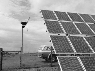
Wind and solar application in the city of Huleka in South Africa.
(SMA Solar Technology AG.)
Furthermore, the solar PV industry is growing very fast, sustaining an annual growth rate of more than 40% for the last decade. Because of this fast growth, decreasing costs, and a vast technical potential, solar energy is becoming an important alternative for the future energy needs. With increasing applications of distributed and utility-scale PV as well as concentrating solar power (CSP), solar technologies start to play an important role in meeting the world’s energy demand.
The term photovoltaic describes the conversion process to convert light energy directly to electric energy. The developments in semiconductor technology cause the invention of the PV cell (also known as solar cell) in the early 1950s.
PV and CSP technologies both use the sun to generate electricity. However, they do it in different ways. The earth’s surface receives sunlight in either a direct or diffuse form. Direct sunlight is solar radiation whose path is directly from the sun’s disk and shines perpendicular to the plane of a solar device. This is the form used by CSP systems and concentrating PV systems, in which the reflection or focusing of the sun’s light is essential to the electricity-generating process. Flat-plate or non-concentrating, PV systems can also use direct sunlight. Figure 13.15 shows solar applications on the roof of Oregon State Capital in Salem, Oregon. Figure 13.16 shows solar installations at Montalto di Castro in Italy. Figure 13.17 shows solar applications on the rooftop of a barn in Bayern, Germany. Figure 13.18 shows solar module used in the city of Kassel in the state of Hessen, Germany. Figure 13.19 shows solar and wind turbine applications in the state of Rheinland-Pfalz in Germany.

Solar applications on the roof of Oregon State Capital, Salem, Oregon, United States.
(SMA Solar Technology AG.)


Solar applications on the rooftop of a barn in Bayern, Germany.
(SMA Solar Technology AG.)

Solar module used in the city of Kassel in the state of Hessen, Germany.
(SMA Solar Technology AG.)

Solar and wind turbine applications in the state of Rheinland-Pfalz in Germany.
(SMA Solar Technology AG.)
PV (or solar electric) systems use semiconductor solar cells to convert sunlight directly into electricity. In contrast, CSP (or solar thermal electric) systems use mirrors to concentrate sunlight and exploit the sun’s thermal energy. This energy heats a fluid that can be used to drive a turbine or piston, hence producing electricity. Succinctly put, PV uses the sun’s light to produce electricity directly, whereas CSP uses the sun’s heat to produce electricity indirectly. Again, PV and CSP both use the sun to produce electricity. However, they use different forms of the sun’s radiation.
Other solar radiation is diffuse, meaning the sunlight reaches the earth’s surface after passing through thin cloud cover or reflecting off of particles or surfaces. Global radiation is the sum of the direct and diffuse components of sunlight. This global radiation, as well as direct or diffuse radiation alone, can be used by flat-plate PV systems to generate electricity.
As said before, PV and CSP are different forms of solar technologies. Similarly, there are different PV materials and designs for generating electricity, which include crystalline silicon, thin films, concentrating PV, and future-generation PV, in addition to associated balance of systems components.
The new technologies, such as depositing solar modules onto a flexible plastic substrate or using solar “inks” (e.g., copper indium gallium selenide) and a “printing” process to produce film solar panels, are ready to drastically reduce the cost of solar power plants to less than $1/W.
Solar power plants can be built where they are most needed in the grid because siting PV arrays is usually much easier than siting a conventional power plant. Also, unlike conventional power plants, modular PV plants can be expanded incrementally as demand increases. It is expected that municipal solar power plants with few megawatt capacity built close to load centers will become common during the next decade.
13.10.2 Crystalline Silicon
Silicon was one of the very first materials that were used in early PV devices, and it still has more than 90% of the market share in today’s commercial solar cell market. The silicon-based cells are known as first-generation PV. Pure silicon is mixed with very small amounts of other elements such as boron and phosphorous, which become positive- and negative-type semiconductor materials, respectively. Putting the two materials in contact with one another creates a built-in potential field.
Thus, when this semiconductor device is subject to the sunlight, the energy of the sunlight frees electrons that then move out of the cell, because of the potential field, into wires that form an electric circuit. Such “PV” effect needs no moving parts and does not use up any of the material in the process of generating electricity. Figure 13.20 shows solar applications on a building in the city of Laatzen in the state of Niedersachsen, Germany. Figure 13.21 shows solar applications in a sports stadium in the city of Mainz in the state of Rheinland-Pfalz in Germany. Figure 13.22 shows solar application in a German school in San Salvador (SMA Solar Technology AG). Figure 13.23 shows solar rooftop applications in the state of Baden-Wurttemberg, Germany.

Solar applications on a building in the city of Laatzen in the state of Niedersachsen, Germany.
(SMA Solar Technology AG.)

Solar applications in a sports stadium in the city of Mainz in the state of Rheinland-Pfalz in Germany.
(SMA Solar Technology AG.)


Solar rooftop applications in the state of Baden-Wurttemberg, Germany.
(SMA Solar Technology AG.)
A typical solar cell has a glass or plastic cover or other encapsulated cover, an antireflective surface layer, a front contact to permit electrons to enter a circuit, and a black contact to permit the semiconductor layers where the electrons start and finish their flow. The thickness of a crystalline silicon (c-Si) cell may be 170–200 pm (10–6).
Figure 13.24 shows a typical 3 in. diameter cell. It will produce a voltage of 0.57 V when sunlight shines upon it under open-circuit conditions. This voltage would be the same regardless of how big the size of the cell is. But its current supply is directly proportional to its surface area. In that sense, a solar cell can be considered a constant current source as well as a voltage source. The solar cell is a nonlinear device and its performance is subject to its characteristic curve.

Figure 13.25 shows a typical I–V characteristic for a PV cell. Note that when the current is zero (i.e., no load), the voltage (i.e., the open-circuit voltage Voc) is about 0.6 V. As the load resistance increases, causing the voltage output of the cell to increase, the current remains relatively constant until the “knee” of the curve is reached. The current then drops off quickly, with only a small increase in voltage, until the open-circuit condition is reached. At this point, the open-circuit voltage is obtained and no current is drawn from the device.
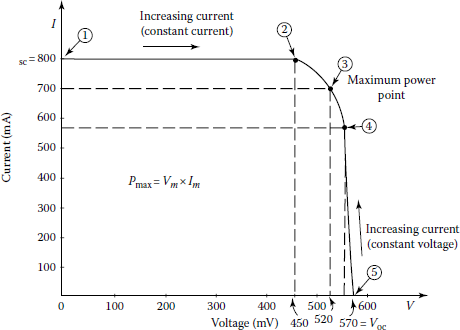
A solar cell will produce a voltage of 0.57 V when the sunlight shines upon it under open-circuit conditions. This voltage would be the same regardless of how big the size of the cell is. But its current supply is directly proportional to its surface area. In that sense, a solar cell can be considered a constant current source as well as a voltage source. The solar cell is a nonlinear device and its performance is subject to its characteristic curve.
The power output of any electrical device, including a solar cell, is the output voltage times the output current under the same conditions. The open-circuit voltage is a point of no power, that is, the current is zero. Similarly, the short-circuit condition produces no power because the voltage is zero. The maximum power point is the best combination of voltage and current. This is the point at which the load resistance matches the solar cell internal resistance.
The power into the cell is a function of the cell area and the power density of light. Once these are fixed, the peak efficiency takes place when the power output is maximum. Thus, the maximum power point should be selected as the operating point of the cell. The maximum power out takes place somewhere around the center of the knee of the curve.
The power into the solar cell is a function of the cell area and the power density of the light. Hence, for a given cell, the peak efficiency takes place when the power output is a maximum. The voltage and current can then be changed electrically to their desired values. In general, the solar cell responds well to all forms of visible light. Thus, they can operate indoors from incandescent or florescent lamps.
The peak power current changes proportionally to the amount of sunlight, but the voltage drops only slightly with large changes in the light intensity. Hence, a solar cell system can be designed to extract enough usable power to trickle-charge a storage battery even on a cloudy day.
It is estimated that the sun is constantly emitting 1.7 × 10²³ kW of power. A very small portion of this (about 8.5 × 10²³ kW) reaches the earth. About 30% of this is lost and 70% (about 6 × 10¹³ kW) penetrates our atmosphere. The amount of power per unit area that is received from the sum is defined as power density. When the sun is directly overhead on a clear day, the power density of sunlight is about 100 mW/cm2. The power density of sunlight is also defined with a unit called the sun. Hence,
On a cloudy day, the power density of sunlight might be
Energy density is another quantity that is also used to measure sunlight. Its unit is the Langley.
Example 13.11
Determine the energy density in Langleys, if the strength of sunshine is 1 sun for a period of 2 min.
Solution
To determine the energy density, use Equation 13.28:
Example 13.12
Assume that the solar cell whose characteristic is shown in Figure 13.25 is connected to a resistive load. Determine the required value of load resistance RL to obtain at each of the operating points of 1, 2, 3, 4, and 5 on the following characteristics:
Solution
At point 1: |
V = 0, |
I = Isc = 800 mA |
At point 2: |
V = 450 mV, |
I = 800 mA |
At point 3: |
V = 700 mV, |
I = 520 mA |
At point 4: |
V = 570 mV, |
I = 550 mA |
At point 5: |
V = 570 mV, |
I = 0 mA |
Example 13.13
Determine the electric power (output power) that can be obtained from the solar cell at each of the points in Example 13.12.
Solution
At point 1: |
P = (0 mV)(800 mA) = 0 W |
At point 2: |
P = (450 mV)(800 mA) = 0.36 W |
At point 3: |
P = (700 mV)(520 mA) = 0.364 W |
At point 4: |
P = (570 mV)(550 mA) = 0.313 W |
At point 5: |
P = (570 mV)(0 mA) = 0 W |
Notice that a good power output is obtained between points 2 and 3. In fact, maximum power output is obtained at the point 3, that is, the maximum power point.
Example 13.14
Determine the energy density in langley, if the strength of sunlight is 1/2 sun for a period of 2 min.
Solution
By using Equation 13.28, the energy density in Langley is
It can be seen that still the same amount of energy density is obtained, but it would take twice as long at 1/2 sun.
Example 13.15
Consider the rooftop of a home measuring 12 m × 15 m that is all covered with PV cells to provide the electric energy requirement by that home. Assume that the sun is at its peak (i.e., having strength of 1 sun) for 3 h every day and the efficiency of a solar cell is 10%. (i.e., 10% of the sunlight power that falls on the cell is converted to electric power.) Determine the average daily electric energy converted by the rooftop.
Solution
The area of the roof is
The amount of power collected by the rooftop is
Since the cells are 10% efficient, the electric power converted by the cells will be
Assuming that a peak sun exists for 2 h every day, the average daily energy is
Example 13.16
Consider the results of Example 13.15 and assume that the cost of electric energy to the homeowner is $0.10/kWh charged by the utility company. If the cost of solar roof is about $5000, determine the following:
- The amount of electric energy produced by solar cells per year
- The amount of savings on electric energy to the homeowner per year
- The break-even period for the solar panels to pay for themselves in months
Solution
- The amount of electric energy produced by the solar panels per year is
- The amount of savings to the homeowner due to electric energy produced by the solar panels per year is
- The break-even time for the solar panels to pay for themselves is
13.10.3 Effect of Sunlight on Solar Cell's Performance
The I–V characteristic given in Figure 13.22 is based on the assumption that the solar cell is operating under a bright noontime sun. In the event that the power density of the sunlight decreases, the output of the cell decreases accordingly. The reasons for such decrease may include the following: The sun is not shining directly on the cell due to the fact that it is just rising or setting; the sun is not shining on the cell because it is winter. (In the northern hemisphere, the sun has a southern exposure. On the other hand, in the southern hemisphere, the opposite is true, that is, in winter, the sun has a northern exposure.) There may exist tall trees or structures that cast a shadow on the cell, during certain times of the day; it is a cloudy or overcast day.
The angular position on the earth’s surface north or south of the equator is defined as the latitude. The equator itself has 0° latitude and divides the earth into two equal hemispheres. For every 69 miles north or south of the equator, the latitude increases by 1°. For instance, the north pole has a latitude of 90° north and the south pole has a latitude of 90° south. Table 13.6 gives the latitudes of selected cities around the world.
Latitudes of Selected Cities around the World
Location |
Latitude |
Location |
Latitude |
|---|---|---|---|
Athens, Greece |
38° N |
Madrid, Spain |
40° N |
Berlin, Germany |
53° N |
Miami, Florida |
26° N |
Bogota, Columbia |
2° N |
Montreal, Canada |
46° N |
Bombay, India |
20° N |
Moscow, Russia |
55° N |
Buenos Aires, Argentina |
20° N |
Munich, Germany |
48° N |
Cairo, Egypt |
30° N |
Oslo, Norway |
60° N |
Edinburgh, Scotland |
56° N |
Paris, France |
49° N |
Entebbe, Uganda |
0° |
Quito, Ecuador |
0° |
Honolulu, Hawaii |
20° N |
Rio de Janeiro, Brazil |
23° S |
Houston, Texas |
30° N |
Rome, Italy |
42° N |
Kansas City, Missouri |
39° N |
Seattle, Washington |
47° N |
Las Vegas, Nevada |
36° N |
Sydney, Australia |
35° S |
Lima, Peru |
12° S |
Thule, Greenland |
77° N |
London, England |
52° N |
Tokyo, Japan |
36° N |
Los Angeles, California |
34° N |
Valparaiso, Chile |
36° N |
Sun’s position varies at a given time. For example, at noontime, the sun’s position varies about 40° from its highest position in June to its lowest position in December. In March and September (equinox), the sun’s center is directly over the equator. Its apparent position in the sky then is approximately equal to your latitude. Thus, in New York City, the noontime sun will appear to be 40° south of vertical during the equinox. In June, it will be 20° (40°–20°) south of vertical, and in December, 60° (40° + 20°) south of vertical.
For maximum energy absorption from the sun, a solar cell should be tilted south (in the northern hemisphere) by the angle of the latitude of the location on the earth.
Example 13.17
At what angle a solar cell should be tilted to get the most energy from the sun if it is located in
- Quito, Ecuador?
- Athens, Greece?
- Valparaiso, Chile?
Solution
It is illustrated in Figure 13.26 below.
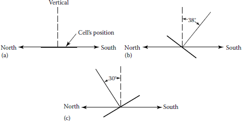
13.10.4 Effects of Changing Strength of the Sun on a Solar Cell
It is often that characteristics of a solar cell include the effects of a variation in power density. The current output of a cell is directly proportional to the sunlight.
Thus, under a very weak sun, the cell puts out very little current. However, its voltage is still quite high. Thus, one can conclude that under open-circuit conditions, the voltage is relatively independent of sunlight. But the effect of the load on the operating point as the power density varies is more important.
Example 13.18
Assume that a fixed resistive load selected to force the solar cell shown in Figure 13.27 operates at the point where maximum power conversion takes place.

- If that point has full sunlight (1 sun), determine the value of the load resistance RL at the maximum power point a in Figure 13.27.
- Determine the value of the power that can be obtained at such point a.
- Let's say due to passing by cloud now, the power density drops to 0.5 sun, and as a result, the operating point of the cell changes. At the corresponding lower sun curve (with the current output of 300 mA and the fixed load resistance), determine the value of the voltage.
- Correspondingly, the new operating point is at b in Figure 13.27. Determine the power at this point.
- Find the new load resistance that is necessary to achieve this.
- As it can be observed from Figure 13.27 that the solar cell is no longer operating at the knee of the curve, consequently, the maximum power is not being converted. To achieve the maximum power conversion, the operating point has to be moved to the point c in Figure 13.27. As a result, there has to be a new load resistance. Determine its value.
- Determine the corresponding power at the point c. (Note that the power at the point c is one-half the power at the point a.)
Solution
- The value of the load resistance is
- The value of the power at such point a is
- The value of the voltage at point a is
- Thus, the power at the new point b is
Consequently, the maximum power is not being converted.
- In order to find the new load resistance that is necessary to achieve the maximum power, the operating point has to be moved to the point c in Figure 13.27.
- As a result, there has to be a new load resistance. Hence,
- Hence, the corresponding power at point c becomes,
Note that the power at the point c is one-half the power at the point a.
Therefore, it can be concluded that the current output is directly proportional to the sunlight (i.e., power density). However, the power will not be proportional unless the load is changed as the intensity of the light varies. Accordingly, the maximum power output of solar cell is a function of not only sunlight but also the load. Because of this, inverters employed for solar energy conversion systems have special tracking circuitry that continuously adjusts the loading on the solar cells while monitoring power output.
The predictability of how much power can be obtained from the sun from hour to hour or day to day is a very serious problem from the scheduling point of view. This problem is also caused by the variation in sunlight. Because of this, it is often that the average data on sunlight are used.
Example 13.19
In order to determine how much energy can be received from the sun by one solar cell in a city in California, data were collected on a sunny day and the data are given in Table 13.7. During the day, the sun rises at 7 AM and sets at 7 PM.
Data for Example 13.19
Power Density (Suns) |
Time (h) |
Energy Density (Sun-Hours) |
|---|---|---|
0.2 |
1 |
0.2 |
1.0 |
1 |
1.0 |
0.9 |
2 |
1.8 |
1.0 |
3 |
3.0 |
0.9 |
2 |
1.8 |
0.3 |
1 |
0.3 |
0.2 |
1 |
0.2 |
0.1 |
1 |
0.1 |
Total = 8.4 sun-h |
Solution
Since from Table 13.7, the total energy density for the day is 8.4 sun-h, it is equivalent to having a full or peak sun (i.e., 1 sun) for 8.4 h. Keeping this in mind and using the power calculated in part (c) for 1 sun power density in Example 13.17,
Thus, the total energy* that can be produced by one solar cell can be found as
13.10.5 Temperature's Effect on Cell Characteristics
The ratings of solar cells are based on the minimum current they supply at 0.45 V under a full sun at 25°C (77°F). Its output is a function of its cell temperature. As temperature increases, the current will increase, while the voltage will decrease by about 2.1 mV/°C. As a result, its power output and consequently its cell efficiency decrease.
The opposite takes place as the temperature decreases; that is, cell operates more efficiently when they are cooler. Because of this, commercially manufactured solar panels, that is, groups of interconnected cells, have a metal (usually, aluminum) that plays the role of a heat sink. Otherwise, in areas of low latitude, the temperatures of a solar cell can reach 80°C (i.e., 176°F) without a heat sink. At other temperatures, the voltage and the current of the cell can be determined from
and
where
- ER and IR are the cell ratings in volts and milliamperes, respectively, at 25°C
- E0 and I0 will be the cell voltage and current at the new temperature T in degrees Celsius
- A is the cell area in square centimeter
Example 13.20
Assume that a solar cell is rated 600 mA, 0.45 V, at 25°C, and that the cell area is 30 cm2. If as the cell is under a full sun and providing maximum power, the temperature increases to about 50°C, determine the following:
- Its power output at 25°C
- Its voltage, current, and power output at 50°C
- The amount of percentage drop in power output due to the increased temperature Solution
Solution
- Its power output at 25°C can be found from its rated voltage and current values as
- From Equation 13.29, its new voltage is
And from Equation 13.30, the new current is
Hence, the new power output of the cell is
- The amount of drop power output in percentage is
Temperature effects have to be considered when a PV system is designed. In general, the power estimate is increased by about 10% to take into account the loss due to increased cell temperature.
13.10.6 Efficiency of Solar Cells
In general, solar cell efficiency is defined as the ratio of the electric power output to the sunlight power it receives. The maximum theoretical efficiency of a silicon solar cell is about 25%. Today’s cells have rated efficiencies of 10%–16%.
The efficiency of a cell is a function of number of things, including the number and thickness of the wires connected to the top of the cell and light reflected from the surface of the cell. Also, when cells are connected together to form panels, the panel efficiency will be based on the cell’s shape. Figure 13.20 shows solar rooftop applications in the state of Baden-Wurttemberg, Germany.
Example 13.21
Consider a circular cell that has a diameter of 2.5 in. If it has a rating at 25°C of 1200 mA and 0.45 V in a full sun, determine the cell's efficiency.
Solution
In order to determine the cell's efficiency, first, let us find the cell area. Since the radius of the cell is
or
then
Since 1 sun = 100 mW/cm2,
Thus, the efficiency is
13.10.7 Interconnection of Solar Cells
Typical solar cell output is 800 mA at 0.45 V. But most everyday applications dictate more than 800 mA at 0.45 V. However, solar cells can be treated just like batteries. The net voltage can be increased by connecting them in series, and the net current can be increased by connecting them in parallel. For instance, if 12 identical cells each rated 1 A and 0.45 V in a full sun are connected, as shown in Figure 13.28, the net output of the system will be 3 A at 1.8 V. For each parallel path, the current increases by 1 A, and for each cell in series, the voltage increases by 0.45 V.
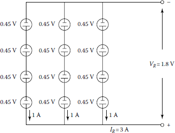
It may be of an interest that solar cells are more flexible than batteries in that they can be broken into pieces to get odd ratings. The voltage output from a piece of a cell will still be the rated voltage of the whole cell. But the current will be proportional to the area of the piece of cell. It is a common practice to cut the circular cells in halves and quadrant cells. If many solar cells are connected in series and parallel to form a permanent unit, it is called a solar panel.
However, the current produced by a series connection of multiple cells will be the minimum of all the cells. For example, if three cells each rated 1 A are connected in series with a half of the same cell (rated 0.5 A), the current will be 0.5 A. In practice, solar panels are manufactured in different sizes and ratings. Such panels can be interconnected to form solar arrays or modules.
Example 13.22
Consider a solar panel that is rated 20 W at 1.0 V. Determine the following:
- How many of these panels are needed to supply 1 A of current at 120 V?
- How should they be connected?
- The value of the necessary load resistance.
- The total power that can be obtained from this array of solar cells.
Solution
- Since each panel produces 12 V, to get 120 V, the number of panels required in series is
- The current rating of each panel can be found from panel's power and voltage ratings. Hence,
Thus, each path, of seriously connected panels, will provide 2 A. Therefore,
Hence, five parallel paths each having 12 panels in series are required to form an array to meet the power requirement. The resultant panel arrangement is shown in Figure 13.29.
- The value of the required load resistance is found as
This input resistance facilitates the maximum power conversion in a full sun. However, as the lighting changes, this input impedance needs to be changed in order to get the maximum power conversion.
- The total power that can be obtained from this solar array is
Alternatively,

13.10.8 Overall System Configuration
PV cells and modules are configurable from 1 to 5 MW. A solar generator has basically two possible fundamental configurations. The first one is a stand-alone system, as shown in Figure 13.30a. It can be used in the location where there is no utility power available. During peak sun-hours, the solar array supplies all the ac power needs and keeps the storage batteries fully charged. The storage batteries have to have the capability of storing enough energy to supply the power required when the sun goes down.

Two fundamental solar generator configurations: (a) stand-alone system and (b) supplemental or cogeneration system.
In the second system, shown in Figure 13.30b, the solar generator is connected to the utility grid. Here, there is no need for the storage batteries. The dc power from the solar array gets inverted to ac power. The inverter output provided the ac power needs, during peak sun-hours. In the event that these needs are low, the power will be fed back into the utility grid for credit. On the other hand, during nighttime hours, the ac power requirements are met by the power supplied by the utility grid. Figure 13.30 only shows the overall system configuration, without the necessary circuit breakers and/or meters.
The overall system frequency must take into account of the effectiveness of all other components (such as inverter, batteries, and any additional circuitry) in addition to the efficiency of the solar array. Figure 13.31 shows a solar module used in the city of Kassel in the state of Hessen, Germany.

Solar module used in the city of Kassel in the state of Hessen, Germany.
(SMA Solar Technology.)
A given solar energy system is designed based on the size of the solar array requirement (for a given specific location and electric energy needs for that location) and the amount of electric energy that the array can supply. After the location and solar array size and its rating are known, the energy output from the system can be easily determined.
Example 13.23
Smith lives in Miami, Florida (with yearly average of 4.7 peak sun-hours per day), and is considering placing a PV array on his south-facing roof. The roof is unshaded and has a size of 25 by 44 ft. The electric power produced is to be converted to ac and used in his home. Any excess power produced will be back into the local utility company's grid system. Analyze the system configuration and determine how much energy Smith can expect to get from the solar installation.
Solution
The system configuration will be like the one shown in Figure 13.30b. But, in addition, there will be a circuit breaker and an ac watt-hour meter will be placed between the inverter and the utility grid. The amount of energy that will be sold to the utility company through the grid connection will be measured by the watt-hour meter. The local utility company by law (PURPA Act of 1078) is obliged to pay for this energy.
The solar panel chosen for this application is rated 16.2 V, 2.4 A, and 39 W and has 10% efficiency at 25°C in full sun. Its dimensions are 1 by 4 ft. At 50°C, the ratings of the solar panel become 14.7 V, 2.27 A, and 55 W. If about 4 ft is permitted at the edges of the roof for a work area, 63 solar panels can easily be placed on the roof. They could be placed end to end with seven in a row (9 × 4 = 36 ft) and nine rows total (9 × 1 = 9 ft), as illustrated in Figure 13.32. Hence, the maximum power output will be

A 3.2 kW single-phase inverter will be employed. Its maximum input current is specified as 25 A, and the input voltage can vary from 60 to 120 V dc. The output voltage is 120 V ac. The seven panels in each row will be connected in series. This will provide a range of voltage (from 25°C to 50°C) of
to
which is within the range of the inverter. The nine rows will be connected in parallel. Hence, the peak current from the solar array (at 50°C) will be
which is within the inverter limit. The panel should be tilted 26° toward south. Since in Miami, Florida, one can expect an average of 4.7 peak sun-hours per day, multiplying it by the peak power output at 50°C will provide the average daily supplied by the solar array. Hence,
If the inverter efficiency is 95%, the average energy produced by the system per day will be
By multiplying this by 30 days, or
or
At 10 cents/kWh, Smith will save about $343/year in electric bills. The solar array would cost
Thus, the break-even point for this investment is
Smart will recover his initial investment in 9.2 years. But if the cost of solar array drops down to $0.50/peak watt (as predicted previously), the investment cost would be
Thus,
At this price, Smart will recover his investment in less than 5 years.
13.10.9 Thin-Film PV
Second-generation PV devices are a more recent development. They are made of layers of semiconductor materials that are much thinner than those in silicon cells. The thickness of a cell is on the order of only 2–3 μm thick,
In the event that silicon is used, it is typically in the form of amorphous (i.e., not crystallized) silicon (a-Si), which has no discernible crystal structure. Also, microcrystalline silicon thin-film devices are being developed. In addition, other thin-film materials have also been developed and commercialized, including cadmium telluride (CdTe) and copper indium gallium diselenide (CIGS). These PV devices need much less material than traditional c-Si devices.
According to Kroposki et al. [9], thin films generally have lower solar conversion efficiency than the c-Si cells. Here, the conversion efficiency is defined as the percentage of the sun’s power shining on the cell. For instance, if 1000 W of solar power illuminates a cell and 150 W of electricity is generated, then the cell has a solar conversion efficiency of 15%.
A commercial silicon cell may have an efficiency of about 20%, whereas a commercial CdTe cell’s efficiency is about 11%. The thin-film cell uses less material and can be deposited with a method that is much less energy intensive than silicon. Less material also causes lighter weight.
Also, some thin-film technologies do not use rigid wafers; instead, they can be deposited on flexible layers of stainless steel or plastic. Depending on the application, such flexibility might be highly desirable. In general, thin-film PV is less expensive to manufacture and easier to implement [8].
13.10.10 Concentrating PV
There is another type of second-generation PV device that is based on high-efficiency multifunction cell that uses compounds from the group III and group V elements of the periodic table of elements. For example, such multifunction solar cell design has three layers, each of which absorbs a different portion of the solar spectrum to use in generating electricity.
The top layer may be made of gallium indium phosphide and the bottom layer of germanium. This type of design may have a high efficiency of about 40%. This is due to the fact that each layer in this design is designed to absorb and use a different portion of the solar spectrum.
But such design is expensive since the group III and V materials are costly to produce. However, the cost can go down substantially, if a relatively inexpensive lens or mirror can be employed to focus sunlight on just a small area of cells [9]. For instance, if a 10 × 10 in. lens focuses this area of incident sun onto a 0.5 × 0.5 in. cell, the concentration factor becomes 400×, that is, 100 m2/0.25 in.2 Thus, such cell with the lens can produce as much power as a 10 × 10 in. cell with lens, but at about 1/400 of the cell cost. Even though, they are not suitable for small projects, concentration systems could be very effective in large power generation for several homes.
13.10.11 PV Balance of Systems
Balance of systems compromises all of the components of a PV system beyond the actual PV module that produces the power. A frame structure is also required toward the sun, to stabilize it in the outer elements, including wind and snow.
PV systems produce dc electricity. Hence, if ac is needed, the balance of systems has to include an inverter. But the inverter decreases the overall system efficiency by an additional 5%-10%. However, the system efficiency can be improved by connecting a tracking system to the solar modules. The trackers can be of single axis or dual axis.
The single-axis trackers aligned with the axis in a north–south direction permit the module to trade the sun’s progress across the sky from east to west during the day. Dual-axis trackers further improve the module’s orientation, permitting the sun to always illuminate the cells perpendicular to the plane of the module. The result is the maximum energy output from the system.
In general, residential and commercial PV systems are directly connected to the grid without energy storage. Including battery energy storage would increase the reliability of the system. Hence, the batteries store excess power that is generated from the PV array to be used later. Figure 13.33 shows solar applications in a sports stadium in the city of Mainz in the state of Rheinland-Pfalz in Germany. Figure 13.34 shows solar application in the Ineco airport in the city of Valencia, Spain.

Solar applications in a sports stadium in the city of Mainz in the state of Rheinland-Pfalz in Germany.
(SMA Solar Technology AG.)

Solar application in the INECO airport in the city of Valencia, Spain.
(SMA Solar Technology AG.)
13.10.12 Types of Conversion Technologies
There are two primary technologies for the conversion of sunlight into electricity. PV cells depend on the use of semiconductor devices for the direct conversion of the solar radiation into electric energy. The typical efficiencies of such commercial crystalline PV cells are in the range of 12%–18%, even though there have been experimental cells built that are capable of over 30%.
The second type of technology is based on solar thermal systems. It is known as CSP. It involves intermediate conversion of solar energy into thermal energy in the form of steam, which in turn is employed to drive a turbogenerator. To have high temperatures, thermal systems invariably use concentrators by the use of mirrors either in the form of parabolic troughs or thermal towers.
But, presently, generation of electricity by either technology is considerably more expensive than traditional means. The CSP systems are essentially categorized based on how the systems collect solar energy. The three basic systems are the linear, tower, and disk systems.
13.10.13 Linear CSP Systems
In such systems, CSP collectors capture the sun’s energy with large mirrors that reflect and focus the sunlight onto a linear receiver tube. Inside the receiver, there is a fluid that is heated by the sunlight and then employed to create superheated steam that causes a turbine to rotate in order to drive a generator to produce electricity.
It is also possible to produce the steam directly in the solar field. Here, no heat exchanger is employed, but the system uses expensive high-pressure piping system in the entire solar field. It has a lower operating temperature.
Essentially, concentrating collector fields in such systems are made of a large number of collectors in parallel rows that are usually aligned in north–south orientation to increase both summertime and annual energy collection. Using its single-axis sun-tracking system, the system facilitates the mirrors to track the sun from east to west during the day, causing the sun to reflect continuously onto the receiver tubes.
Such trough designs can use thermal storage. In that case, the collector field is built oversized in order to heat a storage system during the day that in the evening can be used to produce additional steam to generate electricity.
It is also possible to design the parabolic trough plants as hybrid systems that fuel to supplement the solar output during periods of low solar radiation. In such applications, usually a natural gasfired heater or gas–steam boiler/reheater is used [9].
13.10.14 Power Tower CSP Systems
In such system, several large, flat, sun-tracking mirrors, which are called heliostats, focus sunlight onto a receiver at the top of a tower. The receiver has a heat-transfer fluid that is heated to produce steam. The heated steam in turn is employed in a typical turbine generator to generate electricity. The heat-transfer fluid is usually water/steam although in advanced designs replaced by molten nitrate salt due to its better heat-transfer and energy storage capabilities. Presently, such systems have been developed to produce up to 200 MW of electricity.
13.10.15 Dish/Engine CSP Systems
According to Kroposki et al. [9], these systems generate relatively small amounts (3–25 kW) of electricity with respect to other CSP technologies. Here, a solar concentrator (or dish) collects the solar energy radiating directly from the sun. The resultant beam of concentrated sunlight is reflected onto a thermal receiver that collects the solar heat. The dish is attached on a structure that tracks the sun continuously throughout the day to reflect the highest percentage of sunlight that is possibly onto the thermal receiver.
The power conversion unit is made of the thermal receiver and the engine/generator. The thermal receiver is the interface between the dish and the engine/generator. Its function is to absorb the concentrated beams of solar energy and, after converting them to heat, to transfer this heat to the engine/generator.
The thermal receiver can be made of a bank of tubes with a cooling fluid (hydrogen or helium) that is used as a transfer medium. Other thermal receivers are made of heat pipes, where the boiling and condensing of an intermediate fluid transfers the heat to the engine.
The engine/generator system is the subsystem of the dish/engine CSP system. It takes the heat from the thermal receiver and uses it to produce electricity. Most commonly, a Stirling engine is used as the heat engine. It uses a heated fluid to move pistons and create mechanical power to rotate the shaft of the generator to produce electric power.
The last subsystem of the CSP system is thermal energy storage system. It provides a solution for the curtailed energy production when the sun sets or is blocked by the clouds.
13.10.16 PV Applications
PV cells were first used in power satellites. By the end of the 1990s, PV electric generation was cost competitive with the marginal cost of production with gas turbines. As a result, a number of utilities have introduced utility-interactive PV systems to supply portion of their total customer demand. Figure 13.24 shows solar application in the INECO airport in the city of Valencia, Spain.
Some of these systems have been residential and commercial rooftop systems and other systems have been larger ground-mounted systems. PV systems are classified as utility-interactive (gridconnected) or stand-alone systems.
13.10.16.1 Utility-Interactive PV Systems
Utility-interactive PV systems are categorized by IEEE Standard 929 as small, medium, or large PV systems. Small systems are less than 10 kW, medium systems range from 10 to 500 kW, and large systems are larger than 500 kW. Each size dictates different consideration for the utility interaction.
Since the output of PV modules is dc, it is, of course, necessary to convert this output to ac before connecting it to the grid; it is done by an inverter. It is also called a power conditioning unit (PCU). A typical small utility system of a few kilowatts consists of an array of modules selected by either a total cost or an available roof area. The modules are connected to produce an output voltage ranging from 48 to 300 V, as a function of the dc input requirements of the PCU. One or two PCUs are used to interface the PV output to the utility at 120 V or 120/240 V.
The point of utility connection is the load side of the circuit breaker in the distribution panel of the building of the PV system that is connected on the customer side of the revenue meter. However, medium- and large-scale utility-interactive systems differ from small-scale systems only in the possibility that the utility may dictate different interfacing conditions with respect to disconnect and/ or power quality.
13.10.16.2 Stand-Alone PV Systems
They are used when it is not possible to connect to the utility grid. Examples include water-pumping systems, PV-powered fans, power systems for remote installations, and portable highway signs. Some of them include battery storage to operate the system under sun or no-sun situations.
Problems
- 13.1 Consider a wind turbine that is rated at 100 kW in a 10 m/s wind speed in air at standard conditions. If power output is directly proportional to air density, what is the power output of the wind turbine in a 10 m/s wind speed at an elevation of 2000 m above sea level at a temperature of 20°C?
- 13.2 Consider Example 13.4 and assume that the average wind speed at point a is 10 mph, while at point b is 8 mph. In order to capture 2 kW, determine the blade diameter (d) for a wind turbine operating:
- At point a
- At point b
- 13.3 Consider a wind turbine with blades of 10 ft radius. At the location, wind speed was 5 mph for 3 h and 15 mph for another 3 h time period. Determine the amount of energy that can be intercepted by the wind turbine.
- 13.4 Consider the wind turbine given in Example 13.10 and assume that the wind turbine is 2 MW and is under maintenance 200 h in 1 year out of a total of 8760 h of 1 year. If it is actually produced 4000 MWh due to fluctuations in wind availability, determine the following:
- The availability factor of the wind turbine
- The capacity factor of the wind turbine
- The annual load duration of the wind turbine
- 13.5 Consider Example 13.6 and assume that during an 8 h period, the wind had the following average speeds: 4 mph for 2 h duration, 12 mph for 2 h duration, 17 mph for 1 h duration, and 23 mph for 3 h duration. Determine the resultant electric output for the 8 h period.
- 13.6 Assume that a wind generator whose power curve is shown in Figure 13.9 has a blade diameter of 18 ft. If its power output is at 120 V and 60 Hz, determine the net efficiency of the WECS at a wind speed of 15 mph.
- 13.7 Assume that the wind turbine with three blades in Problem 13.6 has been replaced by one with two blades that is rotating at 90 rpm; find the blade efficiency at a wind speed of 16 mph.
- 13.8 A WECS has a eight-pole 60 Hz three-phase synchronous alternator driven at synchronous speed. The blades have an 8 m diameter and a peak efficiency when the TSR = 5. Determine the transmission gear ratio for peak system efficiency at a wind speed of 6 m/s?
- 13.9 A WECS uses a 6-pole 60 Hz three-phase induction generator. It is excited by a three-phase 60 Hz power line. The blades have 11 m diameter and peak efficiency when the TSR = 6. If the generator efficiency is a maximum at a slip of -3.3%, what should the transmission gear ratio be for peak system efficiency at a wind speed of 5 m/s?
- 13.10 Assume that the WECS shown in Figure 12.9c uses a four-pole three-phase induction machine. The line frequency is 60 Hz and the average wind speed is 15 mph. The blades have a 32 ft diameter and peak efficiency when the TSR = 6. If the generator efficiency is a maximum at a negative slip of 3.3%, determine the transmission gear ratio that is necessary for the peak system efficiency.
- 13.11 Determine the energy density in langleys, if the strength of sunlight is 1 sun for a period of 15 min.
- 13.12 Consider a type of rooftop of a home measuring 15 m × 20 m that is all covered with PV cells to provide the electric energy requirement by that home. If the peak sun per day is 4 h and the efficiency of solar cell is 10%, find the average daily electric energy converted by the rooftop.
- 13.13 Consider the results of Problem 13.12, and assume that the cost of electric energy to the homeowner is $0.19/kWh that is changed by the utility company. If the cost of solar roof is about $5000, determine the following:
- The amount of electric energy produced by the solar cells per year
- The amount of savings on electric energy produced by the solar cells per year
- The break-even period for the solar panels to pay for themselves in months
- 13.14 Consider a circular solar cell that has a 4 in. diameter that is rated 2.0 A at 0.45 V. If a certain application dictates 1.8 V and draws 0.5 A, how can the cell be modified to satisfy the requirements of such application?
- 13.15 A circular cell has a diameter of 3 in. If it has a rating at 25°C of 800 mA and 0.45 V in a full sun, determine its efficiency.
- 13.16 A circular cell has a diameter of 3 in. If it has a rating at 25°C of 1200 mA and 0.45 V in a full sun, determine its efficiency.
- 13.17 Assume that Smart owns a vacation cottage in Napa Valley. He is considering installing a solar system to meet the electricity needs at the cottage. Table P17.1 gives the energy demands at the cottage. Assume that there is five peak sun-hours per day at the location of the cottage.
Necessary Energy Data for the Cottage
Appliance
Current (A)
Time (h)
Battery Drain (A A)
Power (W)
Energy (W · h)
Refrigerator
2
22
44
25
550
Miscellaneous (radio, TV, lighting, toaster, etc.)
5
4
20
75
300
Total
64
100
850
All the electric equipment requires 12 V dc. Design the system and determine the following:
- Design the solar system
- The changing current of the battery for every hour of peak sun
- The size of the battery that is needed
- The peak power of the panels
- If the cost is $1/peak watt, find the cost of panels alone
- 13.18 Consider a solar module rated 5.3 V, 38 W. If it is used to provide power to an application that needs 30 V and 25 A current, determine the following:
- The total number of solar modules required
- The type of connection that is needed in terms of series and parallel connected modules
- The necessary load resistance value to get the rated power
- 13.19 Assume that a roof measures 12 m × 18 m and that the solar array under consideration is 10% efficient and that is tilted 30° toward the south and the yearly average peak sun-hours per day in Dallas, Texas, and Sacramento, California, is 4.7 peak sun-hours and 5 peak sun-hours, respectively. Determine the average daily electric energy converted by the rooftop array, if the house is located at
- Dallas, Texas
- Sacramento, California
References
1. Manwell, J.F., J.G. McGowan, and A.L. Rogers: Wind Energy Explained: Theory, Design, and Application, Wiley, West Sussex, England, 2003.
2. Orloff, S. and A. Flannery: Wind turbine effects on avian activity, habitat use, and mortality in altamont pass and Solano County wind resource areas: 1989–1991, California Energy Commission Report, No. P700–92,002.
3. Stanon, C.: Wind farm visual impact and its assessment, Wind Directions, BWEA, August 1995, pp. 8–9.
4. Wizelius, T.: Developing Wind Power Projects: Theory and Practice, Earthscan, London, U.K., 2007.
5. Smith, J.C. et al.: A mighty wind, IEEE Power Energy Mag., 7(2), March/April 2009, 41–57.
6. Fioravanti, R., V. Khoi, and W. Stadlin: Large-scale solutions, IEEE Power Energy Mag., 7(4), July/ August 2009, 48–57.
7. Grant, W. et al.: Change in the air, IEEE Power Energy Mag., 7(6), November/December 2009, 36–46.
8. Key, T.: Finding a bright spot, IEEE Power Energy Mag., May/June 2009, 34–44.
9. Kroposki, B., R. Margolis, and D. Ton: Harnessing the sun, IEEE Power Energy Mag., May/June 2009, 22–33.
10. Wind Energy: A Vision for Europe in 2030, Report from TPWind Advisory Council, European Wind Energy technology Platform, 2007.
11. Wagner, H.J. and J. Mathur: Introduction to Wind Energy Systems, Springer, Berlin, Germany, 2009.
12. Stanon, C.: Wind farm visual impact and design of wind farms in the landscape, Wind Energy Conversion, 1994, BWEA, pp. 249–255.
13. Gönen, T.: Electric Power Distribution System Engineering, 2nd edn., CRC Press, Boca Raton, FL, 2008, pp. 47–64.
General References
Ackermann, T. et al.: Where the wind blows, IEEE Power Energy Mag., 7(5), November/December 2009, 65–75.
ANSI/IEEE P929, IEEE recommended practice for utility interface of residential and intermediate photovoltaic (PV) systems, IEEE Standards Coordinating Committee 21, Photovoltaics, Draft 10, February 1999.
Babic, J., Walling, R., O’Brien, K., and B. Kroposki: The sun also rises, IEEE Power Energy Mag., May/June 2009, 45–54.
Buresch, M.: Photovoltaic Energy Systems: Design and Installations, McGraw-Hill, New York, 1953.
Denholm, P. and R.M. Margolis: Evaluating the limits of solar photovoltaics (PV) in electric power systems utilizing energy storage and other enabling technology, Energy Policy, 35(9), 2007a, 4424–4433.
Denholm, P. and R.M. Margolis: Evaluating the limits of solar photovoltaics (PV) in traditional electric power systems, Energy Policy, 35(5), 2007b, 3852–2861.
Jha, A.R.: Solar Cell Technology and Applications, CRC Press, Boca Raton, FL, 2010.
Key, T.: Finding a bright spot, IEEE Power Energy Mag., May/June 3009, 34–44.
Komp, R.: Practical Photovoltaics: Electricity from Solar Cells, 3rd edn., Aatec Publications, Ann Arbor, MI, 2002.
Komp, R.J.: Practical Photovoltaics-Electricity from Solar Cells, 2nd edn., Aatce Publications, Ann Arbor, MI, 1984.
Manwell, J.F., J.G. McGowan, and A.L. Rogers: Wind Energy Explained: Theory, Design, and Application, Wiley, West Sussex, England, 2003.
Maycook, P.D. and E.N. Stirewalt: Photovoltaics: Sunlight to Electricity in One Step, Brick House Publishing Company, Andover, MA, 1981.
Mehos, M., Kabel, D., and P. Smithers: Planting the seed, IEEE Power Energy Mag., May/June 2009, 55–62.
Nelson, J.: The Physics of Solar Cells, Imperial College Press, London, U.K., 2003.
Pagliaro, M., Palmisano, G., and R. Criminna: Flexible Solar Cells, Wiley Vch, Weinheim, Germany, 2008.
Stand-Alone Photovoltaic Systems: A Handbook of Recommended Design Practices, Sandia National Laboratories, Albuquerque, NM, 1996.
Stanon, C.: Wind farm visual impact and design of wind farms in the landscape, Wind Energy Conversion, 1994, BWEA, pp. 249–255.
Wind Energy: A Vision for Europe in 2030, Report from TPWind Advisory Council, European Wind Energy technology Platform, 2007.
Wizelius, T.: Developing Wind Power Projects: Theory and Practice, Earthscan, London, U.K., 2007.
Zweibel, K.: Harnessing Solar Power, Plenum Press, New York, 1990.
* It is often that in a classroom, some student who is indeed curious or perhaps just to be smart, Alex asks: “Can we harness lightning as an energy source?” The answer is that lightning is very powerful and very dangerous. But lightning strikes are very brief and infrequent, and therefore, the amount of energy that could be gained (and theoretically stored) would be small in comparison to overall electrical needs. One lightning strike has enough energy (about 1500 MJ) to power a 100 W light bulb for almost half of a year. However, you would need to harness over 58,000 lightning strikes each day to equal the electricity production capability of a large (1 GW) power plant.
* See Gonen [12], Chapter 12.
* Note that a terawatt is denoted as TW so that
- 1 TWh = 1 × 10¹² Wh = 1000 GWh
- T = tera = 1012
- 1 MWh = 1000 kWh
- 1 MW wind power produces 2 GWh/year on land and 3 GWh/year offshore.
* The term grid is often used loosely to describe the totality of the network. For example, grid connected means connected to any part of the electric network. The term national grid usually means the EHV transmission network. Similarly, integration means the physical connection of the generator to the network for secure, safe, and optimal operation of the electrical system.
* An alternative method would be to use a set of curves to the ones in Figure 13.4. Hence, for each power density of the sunlight in Table 13.6, calculate the power at the new of the curve, assuming that the load is adjusted for maximum power. To determine the energy for each time interval, the calculated maximum powers are multiplied by the time of duration. The total energy is found by adding energies for the day.