Chapter 6
Design Considerations of Secondary Systems
Egyptian Proverb: The worst things:
To be in bed and sleep not,
To want for one who comes not,
To try to please and please not.Francis Scott Fitzgerald, Notebooks, 1925
6.1 Introduction
A realistic view of the power distribution systems should be based on “gathering” functions rather than on “distributing” since the size and locations of the customer demands are not determined by the distribution engineer but by the customers. Customers install all types of energy-consuming devices that can be connected in every conceivable combination and at times of customers’ choice. This concept of distribution starts with the individual customers and loads and proceeds through several gathering stages where each stage includes various groups of increasing numbers of customers and their loads. Ultimately the generating stations themselves are reached through services, secondaries, distribution transformers, primary feeders, distribution substations, subtransmission and bulk power stations, and transmission lines.
In designing a system, distribution engineers should consider not only the immediate, that is, short-range, factors but also the long-range problems. The designed system should not only solve the problems of economically building and operating the systems to serve the loads of today but also require a long-range projection into the future to determine the most economical distribution system components and practices to serve the higher levels of the customers’ demands, which will then exist. Therefore, the present design practice should be influenced by the requirements of the future system.
Distribution engineers, who have to consider the many factors, variables, and alternative solutions of the complex distribution design problems, need a technique that will enable them to select the most economical size combination of distribution transformers, secondary conductors, and service drops (SDs).
The recent developments in high-speed digital computers, through the use of computer programs, have provided (1) the fast and economic consideration of many feasible alternatives and (2) the economic and engineering evaluation of these alternatives as they evolve with different strategies throughout the study period. The strategies may include, for example, cutting the secondary, changing the transformers, and possibly adding capacitors.
Naturally, each designed system should meet a specified performance criterion throughout the study period. The most optimum, that is, most economical, system design that corresponds to a load-growth projection schedule can be selected. Also, through the periodic use of the programs, distribution engineers can determine whether strategies adopted continue to be desirable or whether they require some modification as a result of some changes in economic considerations and load-growth projections.
To minimize the secondary-circuit lengths, distribution engineers locate the distribution transformers close to the load centers and try to have the secondary SDs to the individual customers as short as possible.
Since only a small percentage of the total service interruptions are due to failures in the secondary system, distribution engineers, in their system design decisions of the secondary distribution, are primarily motivated by the considerations of economy, copper losses (I2R) in the transformer and secondary circuit, permissible voltage drops, and voltage flicker of the system. Of course, there are some other engineering and economic factors affecting the selection of the distribution transformer and the secondary configurations, such as permissible transformer loading, balanced phase loads for the primary system, investment costs (ICs) of the various secondary system components, cost of labor, cost of capital, and inflation rates.
Distribution transformers represent a significant part of the secondary system cost. Therefore, one of the major concerns of distribution engineers is to minimize the investment in distribution transformers. In general, the present practice in the power industry is to plan the distribution transformer loading on the basis that there should not be excessive spare capacity installed, and transformers should be exchanged, or banked, as the secondary load grows.
Usually, a transformer load management (TLM) system is desirable for consistent loading practices and economical expansion plans. Distribution engineers, recognizing the impracticality of obtaining complete demand information on all customers, have attempted to combine a limited amount of demand data with the more complete, and readily available, energy consumption data available in the customer account files. A typical demand curve is scaled according to the energy consumed, and the resultant information is used to estimate the peak loading on specific pieces of equipment, such as distribution transformers, in which case it is known as TLM, feeders, and substations [3–6].
However, in general, residential, commercial, and industrial customers are categorized in customer files by rate classification only; that is, potentially useful and important subclassifications are not distinguished. Therefore, the demand data are generally collected for the purpose of generating typical curves only for each rate classification.
6.2 Secondary Voltage Levels
Today, the standard (or preferred) voltage levels for the electric power systems are given by the American National Standards Institute’s (ANSI) Standard C84.1-1977 entitled Voltage Ratings for Electric Power Systems and Equipment (60 Hz).
Accordingly, the standard voltage level for single-phase residential loads is 120/240 V. It is supplied through three-wire single-phase services, from which both 120 V lighting and 240 V single-phase power connections are made to large household appliances such as ranges, clothes dryers, and water heaters. For grid- or mesh-type secondary-network systems, used usually in the areas of commercial and residential customers with high-load densities, the voltage level is 208Y/120 V. It is also supplied through three-wire single-phase services, from which both 120 V lighting and 208 V single-phase power connections are made. For “spot” networks used in downtown areas for high-rise buildings with superhigh-load densities and also for areas of industrial and/or commercial customers, the voltage level is 480Y/277 V. It is supplied through four-wire three-phase services, from which both 277 V for fluorescent lighting and other single-phase loads and 480 V three-phase power connections are made.
Today, one can also find other voltage levels in use contrary to the ANSI standards, for example, 120/240 V four wire three phase, 240 V three wire three phase, 480 V three wire three phase, 240/416 V four wire three phase, or 240/480 V four wire three phase.
To increase the service reliability for critical loads, such as hospitals, computer centers, and crucial industrial loads, some backup systems, for example, emergency generators and/or batteries, with automatic switching devices are provided.
6.3 Present Design Practice
The part of the electric utility system that is between the primary system and the consumer’s property is called the secondary system. Secondary distribution systems include step-down distribution transformers, secondary circuits (secondary mains), consumer services (or SDs), and meters to measure consumer energy consumption.
Generally, the secondary distribution systems are designed in single phase for areas of residential customers and in three phase for areas of industrial or commercial customers with high-load densities. The types of the secondary distribution systems include the following:
- The separate-service system for each consumer with separate distribution transformer and secondary connection
- The radial system with a common secondary main, which is supplied by one distribution transformer and feeding a group of consumers
- The secondary-bank system with a common secondary main that is supplied by several distribution transformers, which are all fed by the same primary feeder
- The secondary-network system with a common grid-type main that is supplied by a large number of the distribution transformers, which may be connected to various feeders for their supplies
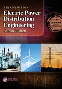
The separate-service system is seldom used and serves the industrial- or rural-type service areas. Generally speaking, most of the secondary systems for serving residential, rural, and light-commercial areas are radial designed. Figure 6.1 shows the one-line diagram of a radial secondary system. It has a low cost and is simple to operate.
6.4 Secondary Banking
The “banking” of the distribution transformers, that is, parallel connection, or, in other words, interconnection, of the secondary sides of two or more distribution transformers, which are supplied from the same primary feeder, is sometimes practiced in residential and light-commercial areas where the services are relatively close to each other, and therefore, the required spacing between transformers is little.
However, many utilities prefer to keep the secondary of each distribution transformer separate from all others. In a sense, secondary banking is a special form of network configuration on a radial distribution system. The advantages of the banking of the distribution transformers include the following:
- Improved voltage regulation
- Reduced voltage dip or light flicker due to motor starting, by providing parallel supply paths for motor-starting currents
- Improved service continuity or reliability
- Improved flexibility in accommodating load growth, at low cost, that is, possible increase in the average loading of transformers without corresponding increase in the peak load
Banking the secondaries of the distribution transformers allows us to take advantage of the load diversity existing among the greater number of consumers, which, in turn, induces a savings in the required transformer kilovolt-amperes. These savings can be as large as 35% according to Lokay [7], depending upon the load types and the number of consumers.
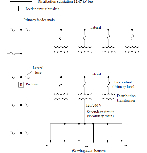
Figure 6.2 shows two different methods of banking secondaries. The method illustrated in Figure 6.2a is commonly used and is generally preferred because it permits the use of a lower-rated fuse on the high-voltage side of the transformer, and it prevents the occurrence of cascading the fuses. This method also simplifies the coordination with primary-feeder sectionalizing fuses by having a lower-rated fuse on the high side of the transformer. Furthermore, it provides the most economical system.
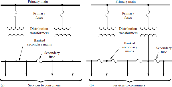
Figure 6.3 gives two other methods of banking secondaries. The method shown in Figure 6.3a is the oldest one and offers the least protection, whereas the method shown in Figure 6.3b offers the greatest protection. Therefore, the methods illustrated in Figures 6.2a and b and 6.3a have some definite disadvantages, which include the following:
- The requirement for careful policing of the secondary system of the banked transformers to detect blown fuses.
- The difficulty in coordination of secondary fuses.
- Furthermore, the method illustrated in Figure 6.2b has the additional disadvantage of being difficult to restore service after a number of fuses on adjacent transformers have been blown.
Today, due to the aforementioned difficulties, many utilities prefer the method given in Figure 6.3b. The special distribution transformer known as the completely self-protecting-bank (CSPB) transformer has, in its unit, a built-in high-voltage protective link, secondary breakers, signal lights for overload warnings, and lightning protection.
CSPB transformers are built in both single phase and three phase. They have two identical secondary breakers that trip independently of each other upon excessive current flows. In case of a transformer failure, the primary protective links and the secondary breakers will both open. Therefore, the service interruption will be minimum and restricted only to those consumers who are supplied from the secondary section that is in fault.
However, all the methods of secondary banking have an inherent disadvantage: the difficulty in performing TLM to keep up with changing load conditions. The main concern when designing a banked secondary system is the equitable load division among the transformers. It is desirable that transformers whose secondaries are banked in a straight line be within one size of each other.
For other types of banking, transformers may be within two sizes of each other to prevent excessive overload in case the primary fuse of an adjacent larger transformer should blow. Today, in general, the banking is applied to the secondaries of single-phase transformers, and all transformers in a bank must be supplied from the same phase of the primary feeder.
6.5 Secondary Networks
Generally speaking, most of the secondary systems are radial designed except for some specific service areas (e.g., downtown areas or business districts, some military installations, hospitals) where the reliability and service-continuity considerations are far more important than the cost and economic considerations. Therefore the secondary systems may be designed in grid- or mesh-type network configurations in those areas.
The low-voltage secondary networks are particularly well justified in the areas of high-load density. They can also be built in underground to avoid overhead (OH) congestion. The OH low-voltage secondary networks are economically preferable over underground low-voltage secondary networks in the areas of medium-load density. However, the underground secondary networks give a very high degree of service reliability. In general, where the load density justifies an underground system, it also justifies a secondary-network system.
Figure 6.4 shows a one-line diagram of a small segment of a secondary network supplied by three primary feeders. In general, the usually low-voltage (208Y/120 V) grid- or mesh-type secondary-network system is supplied through network-type transformers by two or more primary feeders to increase the service reliability. In general, these are radial-type primary feeders. However, the loop-type primary feeders are also in use to a very limited extent. The primary feeders are interlaced in a way to prevent the supply to any two adjacent transformer banks from the same feeder. As a result of this arrangement, if one primary feeder is out of service for any reason (single contingency), the remaining feeders can feed the load without overloading and without any objectionable voltage drop. The primary-feeder voltage levels are in the range of 4.16–34.5 kV. However, there is a tendency toward the use of higher primary voltages.
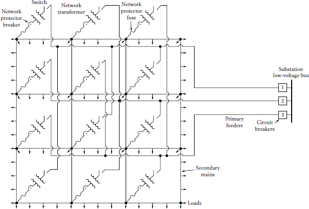
Currently, the 15 kV class is predominating. The secondary network must be designed in such a manner as to provide at least one of the primary feeders as a spare capacity together with its transformers. To achieve even load distribution between transformers and minimum voltage drop in the network, the network transformers must be located accordingly throughout the secondary network.
As explained previously, the smaller secondary networks are designed based upon single contingency, that is, the outage of one primary feeder. However, larger secondary-network systems must be designed based upon double contingency or second contingency, that is, having two feeder outages simultaneously. According to Reps [7], the factors affecting the probability of occurrence of double outages are as follows:
- The total number of primary feeders
- The total mileage of the primary-feeder outages per year
- The number of accidental feeder outages per year
- The scheduled feeder-outage time per year
- The time duration of a feeder outage
Even though theoretically the primary feeders may be supplied from different sources such as distribution substations, bulk power substations, or generating plants, it is generally preferred to have the feeders supplied from the same substation to prevent voltage magnitude and phase-angle differences among the feeders, which can cause a decrease in the capacities of the associated transformers due to improper load division among them. Also, during light-load periods, the power flow in a reverse direction in some feeders connected to separate sources is an additional concern.
6.5.1 Secondary Mains
Seelye [8] suggested that the proper size and arrangement of the secondary mains should provide for the following:
- The proper division of the normal load among the network transformers
- The proper division of the fault current among the network transformers
- Good voltage regulation to all consumers
- Burning off short circuits or grounds at any point without interrupting service
All secondary mains (underground or OH) are routed along the streets and are three phase four wire wye connected with solidly grounded neutral conductor. In the underground networks, the secondary mains usually consist of single-conductor cables, which may be either metallic or nonmetallic sheathed. Secondary cables commonly have been rubber insulated, but PE cables are now used to a considerable extent. They are installed in duct lines or duct banks. Manholes at the street intersections are constructed with enough space to provide for various cable connections and limiters and to permit any necessary repair activities by workers.
The secondary mains in the OH secondary networks usually are open-wire circuits with weatherproof conductors. The conductor sizes depend upon the network-transformer ratings. For a gridtype secondary main, the minimum conductor size must be able to carry about 60% of the full-load current to the largest network transformer. This percentage is much less for the underground secondary mains. The most frequently used cable sizes for secondary mains are 4/0 or 250 kcmil and, to a certain extent, 350 and 500 kcmil.
The selection of the sizes of the mains is also affected by the consideration of burning faults clear. In case of a phase-to-phase or phase-to-ground short circuit, the secondary network is designed to burn itself clear without using sectionalizing fuses or other overload protective devices. Here, “burning clear” of a faulted secondary-network cable refers to a burning away of the metal forming the contact between phases or from phase to ground until the low voltage of the secondary network can no longer support the arc.
To achieve fast clearing, the secondary network must be able to provide for high current values to the fault. The larger the cable, the higher the short-circuit current value needed to achieve the burning clear of the faulted cable. Therefore, conductors of 500 kcmil are about the largest conductors used for secondary-network mains.
The conductor size is also selected keeping in mind the voltage-drop criterion, so that the voltage drop along the mains under normal load conditions does not exceed a maximum of 3%.
6.5.2 Limiters
Most of the time, the method permitting secondary-network conductors to burn clear, especially in 120/208 V, gives good results without loss of service. However, under some circumstances, particularly at higher voltages, for example, 480 V, this method may not clear the fault due to insufficient fault current, and, as a result, extensive cable damage, manhole fires, and service interruptions may occur.
To have fast clearing of such faults, the so-called limiters are used. The limiter is a high-capacity fuse with a restricted copper section, and it is installed in each phase conductor of the secondary main at each junction point. The limiter’s fusing or time–current characteristics are designed to allow the normal network load current to pass without melting but to operate and clear a faulted section of main before the cable insulation is damaged by the heat generated in the cable by the fault current.
The fault should be cleared away by the limiters rapidly, before the network protector (NP) fuses blow. Therefore, the time–current characteristics of the selected limiters should be coordinated with the time–current characteristics of the NPs and the insulation-damage characteristics of the cable.
The distribution engineer’s decision of using limiters should be based upon two considerations: (1) minimum service interruption and (2) whether the saving in damage to cables pays more than the cost of the limiters. Figure 6.5 shows the time–current characteristics of limiters used in 120/208 V systems and the insulation-damage characteristics of the underground-network cables (paper or rubber insulated).
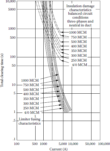
Limiter characteristics in terms of time to fuse versus current and insulation-damage characteristics of the underground-network cables.
(From Westinghouse Electric Corporation, Electric Utility Engineering Reference Book-Distribution Systems, Vol. 3, East Pittsburgh, PA, 1965.)
6.5.3 Network Protectors
As shown in Figure 6.4, the network transformer is connected to the secondary network through an NP. The NP consists of an air circuit breaker with a closing and tripping mechanism controlled by a network master and phasing relay and backup fuses.
All these are enclosed in a metal case, which may be mounted on the transformer or separately mounted. The fuses provide backup protection to disconnect the network transformer from the network if the NP fails to do so during a fault. The functions of an NP include the following:
- To provide automatic isolation of faults occurring in the network transformer or in the primary feeder. For example, when a fault occurs in one of the high-voltage feeders, it causes the feeder circuit breaker, at the substation, to be open. At the same time, a current flows to the feeder fault point from the secondary network through the network transformers normally supplied by the faulted feeder. This reverse power flow triggers the circuit breakers of the NPs connected to the faulty feeder to open. Therefore, the fault becomes isolated without any service interruption to any of the consumers connected to the network.
- To provide automatic closure under the predetermined conditions, that is, when the primary-feeder voltage magnitude and the phase relation with respect to the network voltage are correct. For example, the transformer voltage should be slightly higher (about 2 V) than the secondary-network voltage in order to achieve power flow from the network transformer to the secondary-network system and not the reverse. Also, the low-side transfer voltage should be in phase with, or leading, the network voltage.
- To provide its reverse power relay to be adequately sensitive to trip the circuit breaker with currents as small as the exciting current of the transformer. For example, this is important for the protection against line-to-line faults occurring in unigrounded three-wire primary feeders feeding network transformers with delta connections.
- To provide protection against the reverse power flow in some feeders connected to separate sources. For example, when a network is fed from two different substations, under certain conditions, the power may flow from one substation to the other through the secondary network and network transformers. Therefore, the NPs should be able to detect this reverse power flow and to open. Here, the best protection is not to employ more than one substation as the source.
As previously explained, each network contains backup fuses, one per phase. These fuses provide backup protection for the network transformer if the NP breakers fail to operate.
Figure 6.6 illustrates an ideal coordination of secondary-network protective apparatus. The coordination is achieved by proper selection of time delays for the successive protective devices placed in series. Table 6.1 indicates the required action or operation of each protective equipment under different fault conditions associated with the secondary-network system. For example, in case of a fault in a given secondary main, only the associated limiters should isolate the fault, whereas in case of a transformer internal fault, both the NP breaker and the substation breaker should trip. Figures 6.4 and 6.7 show three-position switches electrically located at the high-voltage side of the network transformers. They are physically mounted on one end of the network transformer.
Required Operation of the Protective Apparatus
Fault Type |
Limiter |
NP Fuse |
NP Breaker |
Substation Circuit Breaker |
|---|---|---|---|---|
Mains |
Yes |
No |
No |
No |
Low-voltage bus |
Yes |
Yes |
No |
No |
Transformer internal fault |
No |
No |
Trips |
Trips |
Primary feeder |
No |
No |
Trips |
Trips |

An ideal coordination of secondary-network overcurrent protection devices.
(From Westinghouse Electric Corporation, Electric Utility Engineering Reference Book-Distribution Systems, Vol. 3, East Pittsburgh, PA, 1965.)
6.5.4 High-Voltage Switch
As shown in Figure 6.7, position 2 is for normal operation, position 3 is for disconnecting the network transformer, and position 1 is for grounding the primary circuit. In any case, the switch is manually operated and is not designed to interrupt current. The first step is to open the primaryfeeder circuit breaker at the substation before opening the switch and taking the network unit out of service. After taking the unit out, the feeder circuit breaker may be closed to reestablish service to the rest of the network.

However, the switch cannot be operated, due to an electric interlock system, unless the network transformer is first de-energized. The grounding position provides safety for the workers during any work on the de-energized primary feeders.
To facilitate the disconnection of the transformer from an energized feeder, sometimes a special disconnecting switch that has an interlock with the associated NP is used, as shown in Figure 6.7. Therefore, the switch cannot be opened unless the load is first removed by the NP from the network transformer.
6.5.5 Network Transformers
In the OH secondary networks, the transformers can be mounted on poles or platforms, depending on their sizes. For example, the small ones (75 or 150 kVA) can be mounted on poles, whereas larger transformers (300 kVA) are mounted on platforms. The transformers are either single-phase or three-phase distribution transformers.
In the underground secondary networks, the transformers are installed in vaults. The NP is mounted on one side of the transformer and the three-position high-voltage switch on the other side. This type of arrangement is called a network unit.
A typical network transformer is three phase, with a low-voltage rating of 216Y/125 V, and can be as large as 1000 kVA. Table 6.2 gives standard ratings for three-phase transformers, which are used as secondary-network transformers. Because of the savings in vault space and in installation costs, network transformers are now built as three-phase units.
Standard Ratings for Three-Phase Secondary-Network Transformers Transformer High Voltage
Preferred Nominal System Voltage |
Rating |
BIL (kV) |
Taps |
Standard kVA Ratings for Low-voltage Rating of 216Y/125 V |
|
|---|---|---|---|---|---|
Above |
Below |
||||
2400/4160Y |
4160a |
60 |
None |
None |
300, 500, 750 |
None |
None |
||||
4330 |
None |
None |
|||
4330Y/2500b |
None |
None |
|||
4800 |
5000 |
60 |
None |
4875/4750/4625/4500 |
300, 500, 750 |
7200 |
7200a |
75 |
None |
7020/6840/6660/6480 |
300, 500, 750 |
7500 |
None |
7313/7126/6939/6752 |
|||
7200 |
11,500 |
95 |
None |
11,213/10,926/10,639/10,w352 |
300, 500, 750, 1000 |
12,000 |
12,000a |
95 |
None |
11,700/11,400/11,100/10,800 |
300, 500, 750, 1000 |
12,500 |
None |
12,190/11,875/11,565/11,250 |
|||
7200/12,470Y |
13,000Y/7500b |
95 |
None |
12,675/12,350/12,025/11,700 |
300, 500, 750, 1000 |
13,200 |
13,200a |
95 |
None |
12,870/12,540/12,210/11,880 |
300, 500, 750, 1000 |
7620/13,200Y |
None |
12,870/12,540/12,210/11,880 |
|||
13,750 |
None |
13,406/13,063/12,719/12,375 |
|||
13,750Y/7940b |
None |
13,406/13,063/12,719/12,375 |
|||
14,440 |
14,400a |
95 |
None |
14,040/13,680/13,320/12,960 |
300, 500, 750, 1000 |
23,000 |
22,900a |
150 |
24,100/23,500 |
22,300/21,700 |
500, 750, 1000 |
24,000 |
25,200/24,600 |
23,400/22,800 |
|||
Source: Westinghouse Electric Corporation, Electric Utility Engineering Reference Book Distribution Systems, Vol. 3, East Pittsburgh, PA, 1965. With permission.
Note: All windings are delta connected unless otherwise indicated.
a Preferred ratings that should be used when establishing new networks.
b High-voltage and low-voltage neutrals are internally connected by a removable link.
In general, the network transformers are submersible and oil or askarel cooled. However, because of environmental concerns, askarel is not used as an insulating medium in new installations anymore. Depending upon the locale of the installation, the network transformers can also be ventilated dry type or sealed dry type and submersible.
6.5.6 Transformer Application Factor
Reps [7] defines the application factor as “the ratio of installed network transformer to load.” Therefore, by the same token,
Application factor=∑ST∑SL(6.1)
where
∑STis the total capacity of network transformers
∑SLis the total load of secondary network
The application factor is based upon single contingency, that is, the loss of one of the primary feeders. According to Reps [7], the application factor is a function of the following:
- The number of primary feeders used
- The ratio of ZM/ZT, where ZM is the impedance of each section of secondary main and ZT is the impedance of the secondary-network transformer
- The extent of nonuniformity in load distribution among the network transformers under the single contingency
Figure 6.8 gives the plots of the transformer application factor versus the ratio of ZM/ZT for different numbers of feeders. For a given number of feeders and a given ZM/ZT ratio, the required capacity of network transformers to supply a given amount of load can be found by using Figure 6.8.
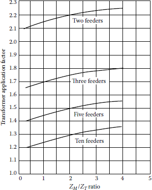
Network-transformer application factors as a function of ZM/ZT ratio and number of feeders used.
(From Westinghouse Electric Corporation, Electric Utility Engineering Reference Book-Distribution Systems, Vol. 3, East Pittsburgh, PA, 1965.)
6.6 Spot Networks
A spot network is a special type of network that may have two or more network units feeding a common bus from which services are tapped. The transformer capacity utilization is better in the spot networks than in the distributed networks due to equal load division among the transformers regardless of a single-contingency condition.
The impedance of the secondary main, between transformers, is zero in the spot networks. The spot networks are likely to be found in new high-rise commercial buildings. Even though spot networks with light loads can utilize 208Y/120 V as the nominal low voltage, the commonly used nominal low voltage of the spot networks is 480Y/277 V. Figure 6.9 shows a one-line diagram of the primary system for the John Hancock Center.
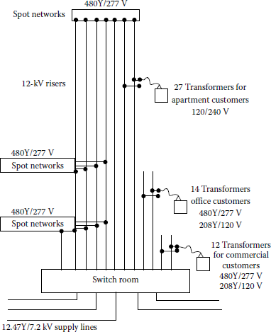
One-line diagram of the multiple primary system for the John Hancock Center.
(From Westinghouse Electric Corporation, Electric Utility Engineering Reference Book-Distribution Systems, Vol. 3, East Pittsburgh, PA, 1965.)
6.7 Economic Design of Secondaries
In this section, a method for (at least approximately) minimizing the total annual cost (TAC) of owning and operating the secondary portion of a three-wire single-phase distribution system in a residential area is presented. The method can be applied either to OH or underground residential distribution (URD) construction. Naturally, it is hoped that a design for satisfactory voltage-drop and voltage-dip performance will agree at least reasonably well with the design that yields minimum TAC.
6.7.1 Patterns and Some of the Variables
Figure 6.10 illustrates the layout and one particular pattern having one span of secondary line (SL) each way from the distribution transformer. The system is assumed to be built in a straight line along an alley or along rear lot lines. The lots are assumed to be of uniform width d so that each span of SL is of length 2d. If SLs are not used, then there is a distribution transformer on every pole and OH construction, and every transformer supplies four SDs.

The primary line, which obviously must be installed along the alley, is not shown in Figure 6.10. The number of spans of SLs each way from a transformer is an important variable. Sometimes no SL is used in high-load density areas. In light-load density areas, three or more spans of SL each way from the transformer may be encountered in practice.
If Figure 6.10 represents an OH system, the transformer, with its arrester(s) and fuse cutout(s), is pole mounted. The SL and the SD may be of either open-wire or triplex cable construction. If Figure 6.10 represents a typical URD design, the transformer is grade mounted on a concrete slab and completely enclosed in a grounded metal housing, or else it is submersibly installed in a hole lined with concrete, Transite, or equivalent material. Both SL and SDs are triplexed or twin concentric neutral direct-burial cable laid in narrow trenches, which are backfilled after the installation of the cable. The distribution transformers have the parameters defined in the following:
- ST is the transformer capacity, continuously rated kVA.
- Iexc is the per unit exciting current (based on ST).
- PT,Fe is the transformer core loss at rated voltage and rated frequency, kW.
- PT,Cu is the transformer copper loss at rated kVA load, kW.
The SL has the parameters defined in the following:
- ASL is the conductor area, kcmil.
- ρ is the conductor resistivity, (Ω· cmil)/ft.
- = 20.5 at 65°C for aluminum cable.
The SDs have the parameters ASD and ρ with meanings that correspond to those given for SLs.
6.7.2 Further Assumptions
- All secondaries and services are single phase three wire and nominally 120/240 V.
- Perfectly balanced loading obtains in all three-wire circuits.
- The system is energized 100% of the time, that is, 8760 h/year.
- The annual loss factor is estimated by using Equation 2.40a, that is,
FLS=0.3FLD+0.7F2LD(2.40a)
- The annual peak-load kilovolt-ampere loading in any element of the pattern, that is, SD, section of SL, or transformer, is estimated by using the maximum diversified demand of the particular number of customers located downstream from the circuit element in question. This point is illustrated later.
- Current flows are estimated in kilovolt-amperes and nominal operating voltage, usually 240 V.
- All loads have the same (and constant) power factor.
6.7.3 General Tac Equation
The TAC of owning and operating one pattern of the secondary system is a summation of investment (fixed) costs (ICs) and operating (variable) costs (OCs). The costs to be considered are contained in the following equation:
TAC=∑ICT+∑ICSL+∑ICSD+∑ICPH+∑OCexc+∑OCT,Fe+∑OCT,cu+∑OCSL,cu+∑OCSD,cu(6.2)
The summations are to be taken for the one standard pattern being considered, like Figure 6.10, but modified appropriately for the number of spans of SL being considered. It is apparent that the TAC so found may be divided by the number of customers per pattern so that the TAC can be allocated on a per customer basis.
6.7.4 Illustrating the Assembly of Cost Data
The following cost data are sufficient for illustrative purposes but not necessarily of the accuracy required for engineering design in commercial practice. Some of the cost data given may be quite inaccurate because of recent, severe inflation. The data are intended to represent an OH system using three-conductor triplex aluminum cable for both SLs and SDs. The important aspect of the following procedures is the finding of equations for all costs so that analytical methods can be employed to minimize the TAC:
- ICT is the annual installed cost of the distribution transformer + associated protective equipment
=(250+7.26×ST)×i $/transformer(6.3)
where
15 kVA≤ST≤100 kVA
ST is the transformer-rated kVA
- ICSL is the annual installed cost of triplex aluminum SL cable
=(60+4.50×ASL)×i $/1000 ft(6.4)
where
ASL is the conductor area, kcmil
i is the pu fixed charge rate on investment
Note that this cost is 1000 ft of cable, that is, 3000 ft of conductor.
- ICSD is the annual installed cost of triplex aluminum SD cable
=(60+4.50×ASD)×i $/1000 ft(6.5)
In this example, Equations 6.4 and 6.5 are alike because the same material, that is, triplex aluminum cable, is assumed to be used for both SL and SD construction.
- ICPH is the annual installed cost of pole and hardware on it but excluding transformer and transformer protective equipment
=$160×i $/pole(6.6)
In case of URD design, the cost item ICPH would designate the annual installed cost of a secondary pedestal or manhole.
- OCexc is the annual operating cost of transformer exciting current
=Iexc×ST×ICcap×i $/transformer(6.7)
where
ICcap is the total installed cost of primary-voltage shunt capacitors = $5.00/kvar
Iexc is the an average value of transformer exciting current based on ST kVA rating = 0.015 pu
- OCT,Fe is the annual operating cost of transformer due to core (iron) losses
=(ICsys×i+8760×ECoff)PT,Fe $/transformer (6.8)
where
ICsys is the average investment cost of power system upstream, that is, toward generator, from distribution transformers
= $350/kVA
ECoff is the incremental cost of electric energy (off-peak)
= $0.008/kWh
PT, Fe is the annual transformer core loss, kW
= 0.004 × ST 15 kVA ≤ ST ≤ 100 kVA
- OCT, Cu is the annual operating cost of transformer due to copper losses
=(ICsys×i+8760×ECon×FLS)(SmaxST)2×PT,cu $/transformer(6.9)
where
ECon is the incremental cost of electric energy (on-peak)
= $0.010/kWh
Smax is the annual maximum kVA demand on transformer
PT,Cu is the transformer copper loss, kW at rated kVA load
=0.073+0.00905×ST where 15 kVA≤ST≤100 kVA(6.10)
FLS is the annual loss factor
- OCSL,Cu is the annual operating cost of copper loss in a unit length of SL
=(ICsys×i+8760 × ECon×FLS)PSL,cu(6.11)
where
PSL,Cu is the power loss in a unit of SL at time of annual peak load due to copper losses, kW
PSL,Cu is an I2R loss, and it must be related to conductor area ASL with R = ρL/ASL
One has to decide carefully whether L should represent length of conductor or length of cable. When establishing ∑OCSL,cu for the particular pattern being used, one has to remember that different sections of SLs may have different values of current and, therefore, different PSL,Cu.
- OCSD,Cu is the annual operating cost of copper loss in a unit length of SD. OCSD,Cu is handled like OCSL,Cu as described in Equation 6.11. When developing ∑OCSD,cu, it is important to relate PSD,Cu properly to the total length of SDs in the entire pattern.
6.7.5 Illustrating the Estimation of Circuit Loading
The simplifying assumptions (5) and (6) earlier describe one method for estimating the loading of each element of the pattern. It is important to find reasonable estimates for the current loads in each SD, in each section of SL, and in the transformer so that reasonable approximations will be used for the copper-loss costs OCT,Cu, ∑OCSL,cu, and ∑OCSD,cu.
To proceed, it is necessary to have data for the annual maximum diversified kilovolt-ampere demand per customer versus the number of customers being diversified. The illustrative data tabulated in Table 6.3 have been taken from Lawrence, Reps, and Patton’s paper entitled Distribution System Planning through Optimized Design, I-Distribution Transformers and Secondaries [13, Fig. 3]. As explained in that paper, the maximum diversified demand data were developed with the appliance diversity curves and the hourly variation factors.
Illustrative Load Data
No. of Customers Being Diversified |
Ann. Max. Demand (kVA/Custoner) |
|---|---|
1 |
5.0 |
2 |
3.8 |
4 |
3.0 |
8 |
2.47 |
10 |
2.2 |
20 |
2.1 |
30 |
2.0 |
100 |
1.8 |
Source: Lawrence, R.F. et al., AIEE Trans., PAS-79(pt. III), 199, June 1960, Fig. 3.
It is apparent that the data could be plotted and the demand per customer for intermediate numbers of customers could then be read from the curve. Alternately, if a digital computer is programmed to perform the work described here, a linear interpolation might reasonably be used to estimate the per customer demand for intermediate numbers of customers.
Figure 6.11 shows a pattern having two SLs each way from the transformer. The reader can apply the foregoing data and with linear interpolation find the flows shown in Figure 6.11. The nominal voltage used is 240 V.

6.7.6 Developed Total Annual Cost Equation
Upon expanding all the cost items (1)–(9) in Section 6.7.4, taking the correct summations for the pattern being used, and introducing the results into Equation 6.2, one finds that
TAC = A+BS2T+CST+D×ST+E×ASD+FASD+G×ASL+HASL(6.12)
where the coefficients A to H are numerical constants. It is important to note that TAC has been reduced to a function of three design variables, that is,
TAC = f(ST,ASD, and ASL)(6.13)
However, one has to remember that many parameters, such as the fixed charge rate i, transformer core and copper losses, and installed costs of poles and lines, are contained in coefficients A to H. It should be further noted that the variables ST, ASD, and ASL are in fact discrete variables. They are not continuous variables. For example, if theory indicates that ST = 31 kVA is the optimum transformer size, the designer must choose rather arbitrarily between the standard commercial sizes of 25 and 37.5 kVA. The same ideas apply to conductor sizes for ASL and ASD.
6.7.7 Minimization of the Total Annual Costs
One may commence by using Equation 6.12, taking three partial derivatives, and setting each derivative to zero:
The work required by Equation 6.14 is formidable. The roots of a cubic must be found. At this point, one has the minimum TAC if only ST is varied and similarly for only ASL and ASD variables. There is no assurance that the true, grant minimum of TAC will be achieved if the results of Equations 6.14 through 6.16 are applied simultaneously.
Having in fact discrete variables in this problem, one now discards continuous variable methods. The results of Equations 6.14 through 6.16 are used henceforth merely as indicators of the region that contains the minimum TAC achievable with standard commercial equipment sizes. The problem is continued by computing TAC for the standard commercial sizes of equipment nearest to the results of Equations 6.14 through 6.16 and then for one (or more?) standard sizes both larger and smaller than those indicated by Equations 6.14 through 6.16.
The results at this point are a reasonable number of computed TAC values, all close to the idealized, continuous variable TAC. Designers can easily scan these final few TAC results and select the (ST, ASL, and ASD) combinations that they think best.
6.7.8 Other Constraints
There are additional criteria that must be met in the total design of the distribution system, whether or not minimum TAC is realized. The further criteria involve quality of utility service. Minimum TAC designs may be encountered, which will violate one or more of the commonly used criteria:
- A minimum allowable steady-state voltage at the most remote service entrance may have been set by law, public utility commission order, or company policy.
- A maximum allowable motor-starting voltage dip at the most remote service entrance similarly may have been established.
- Ordinarily, the ampacity of no section of SLs or SDs should be exceeded by the designer.
- The maximum allowable distribution transformer loading, in per unit of the transformer continuous rating, should not be exceeded by the designer.
Example 6.1
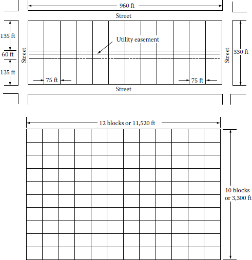
This example deals with the costs of a single-phase OH secondary distribution system in a residential area. Figures 6.12 and 6.13 show the layouts and the service arrangement to be considered. Note that equal lot widths, hence uniform load spacings, are assumed. All SDs are assumed to be 70 ft long. The calculations should be done for one block of the residential area.
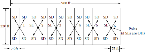
In case of OH secondary distribution system, assume that there are 12 services per transformers, that is, there are two transformers per block that are at poles 2 and 5, as shown in Figure 6.12.
Subsequent problems of succeeding chapters will deal with the voltage-drop constraints, which are used to set a minimum standard of quality of service. Naturally, it is hoped that a design for satisfactory voltage-drop performance will agree at least reasonably well with the design for minimum TAC.
Table 6.4 gives load data to be used in this example problem. Use 30 min annual maximum demands for customer class 2 for this problem.
Load Data for Example 6.1
No. of Customers Being Diversified |
30 Min Ann. Max. Demands (kVA/Customer) |
||
|---|---|---|---|
Class 1 |
Class 2 |
Class 3 |
|
1 |
18.0 |
10.0 |
2.5 |
2 |
14.4 |
7.6 |
1.8 |
4 |
12.0 |
6.0 |
1.5 |
12 |
10.0 |
4.4 |
1.2 |
100 |
8.4 |
3.6 |
1.1 |
Source: Fink, D.G. and Beaty, H.W., Standard Handbook for Electrical Engineers, 11th edn., McGraw-Hill, New York, 1978, Figure 3.
Note: The kilovolt-ampere demands cited have been doubled arbitrarily in an effort to modernize the data. It is explained in the reference cited that the original maximum demand data were developed from appliance diversity curves and hourly variation factors.
Use the following data and assumptions:
- All secondaries and services are single phase three wire, nominally 120/240 V.
- Assume perfectly balanced loading in all single-phase three-wire circuits.
- Assume that the system is energized 100% of the time, that is, 8760 h/year.
- Assume the annual load factor to be FLD = 0.35.
- Assume the annual loss factor to be
- Assume that the annual peak-load copper losses are properly evaluated by applying the given class 2 loads as
- One consumer per SD
- Four consumers per section of SL
- Twelve consumers per transformer
Here, PSL,Cu is an I2R. loss, and it must be related to conductor area ASL with
where
ASL is the conductor area, kcmil
ρ is 20.5 (Ω · cmil)/ft at 65°C for aluminum cable
L is the length of conductor wire involved (not cable length)
(The designer must be careful to establish a correct relation between , that is, the annual OC per block, and the amount of SL for which PSL,Cu is evaluated.)
- Assume nominal operating voltage of 240 V when computing currents.
- Assume a 90% power factor for all loads.
- Assume a fixed charge (capitalization) rate of 0.15.
Using the given data and assumptions, develop a numerical TAC equation applicable to one block of these residential areas for the case of 12 services per transformer, that is, two transformers per block. The equation should contain the variables of ST, ASD, and ASL. Also determine the following:
- The most economical SD size (ASD) and the nearest larger standard AWG wire size
- The most economical SL size (ASL) and the nearest larger standard AWG wire size
- The most economical distribution transformer size (ST) and the nearest larger standard transformer size
- The TAC per block for the theoretically most economical sizes of equipment
- The TAC per block for the nearest larger standard commercial sizes of equipment
- The TAC per block for the nearest larger transformer size and for the second larger sizes of ASD and ASL
- Fixed charges per customer per month for the design using the nearest larger standard commercial sizes of equipment
- The variable (operating) costs per customer per month for the design using the nearest larger standard commercial sizes of equipment
Solution
From Equation 6.2, the TAC is
Since there are two transformers per block and 12 services per transformer, from Equation 6.3, the annual installed cost of the two distribution transformers and associated protective equipment is
From Equation 6.4, the annual installed cost of the triplex aluminum cable used for 300 ft per transformer (since there is 150 ft SL at each side of each transformer) in the SLs is
From Equation 6.5, the annual installed cost of triplex aluminum 24 SDs per block (each SD is 70 ft long) is
From Equation 6.6, the annual cost of pole and hardware for the six poles per block is
From Equation 6.7, the annual OC of transformer exciting current per block is
From Equation 6.8, the annual OC of core (iron) losses of the two transformers per block is
From Equation 6.9, the annual OC of transformer copper losses of the two transformers per block is
where
Here, the figure of 4.4 kVA/customer is found from Table 6.4 for 12 class 2 customers.
From Equation 6.10, the transformer copper loss in kilowatts at rated kilovolt-ampere load is found as
Therefore,
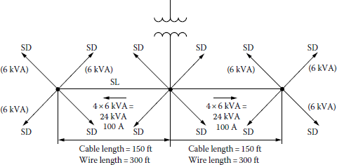
From Equation 6.11, the annual OC of copper losses in the four SLs is
where PLS,Cu is the copper losses in two SLs at time of annual peak load, kW/transformer (see Figure 6.14) = I2 × R
where
Thus,
Also from Equation 6.11, the annual OC of copper losses in the 24 SDs is
where PSD,Cu is the copper losses in the 24 secondary drops at the time of annual peak load, kW
where
From Table 6.4, the 30 min annual maximum demand for one SD per one class 2 customer can be found as 10 kVA. Therefore,
Thus,
Substituting Equations 6.17 through 6.25 into Equation 6.2, the TAC equation can be found as
After simplifying,
- By partially differentiating Equation 6.26 with respect to ASD and equating the resultant to zero,
from which the most economical service-drop size can be found as
Therefore, the nearest larger standard AWG wire size can be found from the copper-conductor table (see Table A.1) as 1/0, that is, 106,500 cmil.
- Similarly, the most economical SL size can be found from
as
Therefore, the nearest larger AWG wire size is 4/0, that is, 211.6 kcmil.
- The most economical distribution transformer size can be found from
or
Therefore, the nearest larger standard transformer size is 50 kVA.
- By substituting the found values of ASD, ASL, and ST into Equation 6.26, the TAC per block for the theoretically most economical sizes of equipment can be found as
- By substituting the found standard values of ASD, ASL, and ST into Equation 6.26, the TAC per block for the nearest larger standard commercial sizes of equipment can be found as
- The second larger sizes of ASD and ASL are 133.1 kcmil and 250 kcmil, respectively. Therefore,
- The fixed charges per customer per month for the design using the nearest larger standard commercial sizes of equipment is
- The variable (operating) cost per customer per month for the design using the nearest larger standard commercial sizes of equipment is
Note that the fixed charges are larger than the OCs.
6.8 Unbalanced Load and Voltages
A single-phase three-wire circuit is regarded as unbalanced if the neutral current is not zero. This happens when the loads connected, for example, between line and neutral, are not equal. The result is unsymmetrical current and voltages and a nonzero current in the neutral line. In that case, the necessary calculations can be done by using the method of symmetrical components.
Example 6.2
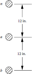
This example and Examples 6.3 and 6.4 deal with the computation of voltages in unbalanced single-phase three-wire secondary circuits, as shown in Figure 6.15. Here, both the mutual-impedance methods and the flux-linkage methods are applicable as alternative methods for computing the voltage drops in the SL. This example deals with the computation of the complex linkages due to the line currents in the conductors a, b, and n. Assume that the distribution transformer used for this single-phase three-wire distribution is rated as 7200/120–240 V, 25 kVA, and 60 Hz, and the n1 and n2 turn ratios are 60 and 30. As Figure 6.15 suggests, the two halves of the lowvoltage winding of the distribution transformer are independently loaded with unequal secondary loads. Therefore, the single-phase three-wire secondaries are unbalanced. The vertical spacing between the secondary wires is as illustrated in Figure 6.16. Assume that the secondary wires are made of #4/0 seven-strand hard-drawn aluminum conductors and 400 ft of line length. Use 50°C resistance in finding the line impedances.

Furthermore, assume that (1) the load impedances and are independent of voltage, (2) the primary-side voltage is and is maintained constant, and (3) the line capacitances and transformer exciting current are negligible. Use the given information and develop numerical equations for the phasor expressions of the flux linkages in terms of and . In other words, find the coefficient matrix, numerically, in the equation
Solution
The phasor expressions of the complex flux linkages due to the line currents in the conductors a, b, and n can be written as*
Since
the current in the neutral conductor can be written as
Thus, substituting Equation 6.32 into Equations 6.28 through 6.30,
Therefore, from Equations 6.33 through 6.35,
Thus, from Equation 6.36, the coefficient matrix can be found numerically as
Note that the elements in the coefficient matrix can be converted to weber-teslas per foot if they are multiplied by 0.3048 m/ft.
Example 6.3
Assume that, in Example 6.2, , , and are specified but not the load impedances and .Develop symbolic equations that will give solutions for the load voltages , , and in terms of the voltage , the impedances, and the flux linkages.
Solution
Since the transformation ratio of the distribution transformer is
the primary-side current can be written as
Here,
Substituting Equation 6.37 into Equation 6.38,
Also,
Substituting Equation 6.39 into Equation 6.40,
By writing a loop equation for the secondary side of the equivalent network of Figure 6.15,
Substituting Equation 6.41 into Equation 6.42,
or
Also, by writing a second loop equation,
Substituting Equation 6.41 into Equation 6.45,
However, from Figure 6.15,
Therefore, substituting Equations 6.43 and 6.45 into Equation 6.46,
Example 6.4
Assuming that in Example 6.3 the given voltages are
and the load impedances are
and
determine the following:
- The secondary currents and
- The secondary neutral current
- The secondary voltages and
- The secondary voltage
Solution
From Equation 6.43,
or
Similarly, from Equation 6.45,
or
Substituting the given values into Equation 6.48,
or
Also, substituting the given values into Equation 6.49,
or
Therefore, from Equations 6.50 and 6.51,
By solving Equation 6.52,
- From Equation 6.53, the secondary currents are
and
- Therefore, the secondary neutral current is
- The secondary voltages are
and
- Therefore, the secondary voltage is
Example 6.5
Figure 6.17 shows an ac secondary network, which has been adapted from Ref. [7]. The loads shown in Figure 6.17 are in three-phase kilowatts and kilovars, with a lagging power factor of 0.85. The nominal voltage is 208 V. All distribution transformers are rated 500 kVA three phase, with 4160 V delta high voltage and 125/216 V wye grounded low voltage. They have leakage impedance ZT of 0.0086 + j0.0492 pu based on transformer ratings.

(Adapted from Westinghouse Electric Corporation, Electric Utility Engineering Reference Book-Distribution Systems, Vol. 3, East Pittsburgh, PA, 1965.)
All secondary underground mains have copper 3-#4/0 per phase and 3-#3/0 neutral cables in nonmagnetic conduits. The positive-sequence impedance ZM of 500 ft of main is 0.181 + j0.115 pu on a 1000 kVA base.
All primary-feeder circuits are 1.25 min long. Three single-conductor 500 kcmil 5 kV shieldedcopper PE-insulated underground cables are used at 90° conductor temperature. Their impedances within the small area of the network are neglected. The positive-sequence impedance ZF of the feeder cable is 0.01 + j0.017 pu on a 1000 kVA base for 1.25 min long feeders. The approximate ampacities are 473 A for one circuit per duct bank and 402 A for four equally loaded circuits per duct bank.
The bases used are (1) three-phase power base of 1000 kVA; (2) for secondaries, 125/216 V, 2666.7 A, and 0.04687 Ω; and (3) for primaries, 2400/4160 V, 138.9 A, and 17.28 Ω.
The standard 125/216 V network-capacitor sizes used are 40, 80, and 120 kvar. In this study, these capacitors are not switched. Ordinarily, it is desired that distribution circuits not get into leading power factor operation during off-peak load periods. Therefore, the total magnetizing vars generated by unswitched shunt capacitors should not exceed the total magnetizing vars taken by the off-peak load. In this example, the total reactive load is 3150 kvar at peak load, and it is assumed that off-peak load is one-third of peak load, or 1050 kvar. Therefore, a total capacitor size of 960 kvar has been used. It has been distributed arbitrarily throughout the network in standard sizes but with the larger capacitor banks generally being located at the larger-load buses and at the ends of radial stubs from the network.
Using the given data, four separate load flow solutions have been obtained for the following operating conditions in the example secondary network:
- Case 1: Normal switching: Normal loads and all shunt capacitors are off.
- Case 2: Normal switching: Normal loads and all shunt capacitors are on.
- Case 3: First-contingency outage: Primary feeder 1 is out. Normal loads and all shunt capacitors are on.
- Case 4: Second-contingency outage: Primary feeders 1 and 4 are out. Normal loads and all shunt capacitors are on. Note that this second-contingency outage is very severe, causing the largest load (at bus 5) to lose two-thirds of its transformer capacity.
To make a voltage study, Table 6.5 has been developed based on the load flow studies for the four cases. The values given in the table are per unit bus voltage values. Here, the buses selected for the study are the ones located at the ends of radials or else the ones that are badly disturbed by the second-contingency outage of case 4.
Bus Voltage Value (pu)
Buses |
Case 1 |
Case 2 |
Case 3 |
Case 4 |
|---|---|---|---|---|
A |
0.951 |
0.967 |
0.954 |
0.915 |
B |
0.958 |
0.975 |
0.955 |
0.860 |
C |
0.976 |
0.986 |
0.966 |
0.873 |
J |
0.959 |
0.976 |
0.954 |
0.864 |
K |
0.974 |
0.984 |
0.962 |
0.875 |
N |
0.958 |
0.973 |
0.963 |
0.924 |
P |
0.960 |
0.977 |
0.966 |
0.926 |
R |
0.945 |
0.954 |
0.938 |
0.890 |
S |
0.964 |
0.972 |
0.951 |
0.898 |
Use the given data and determine the following:
- If the lowest "favorable" and the lowest "tolerable" voltages are defined as 114 and 111 V, respectively, what are the pu voltages, based on 125 V, that correspond to the lowest favorable voltage and the lowest tolerable voltage for nominally 120/208Y systems?
- List the buses given in Table 6.5, for the first-contingency outage, that have (1) less than favorable voltage and (2) less than tolerable voltage.
- List the buses given in Table 6.5, for the second-contingency outage, that have (1) less than favorable voltage and (2) less than tolerable voltage.
- Find ZM/ZT, 1/2(ZM/ZT), and using Figure 6.8, find the value of the "application factor" for this example network and make an approximate judgment about the sufficiency of the design of this network.
Solution
- The lowest favorable voltage in per unit is 114 V:
and the lowest tolerable voltage in per unit is
- There are no buses in Table 6.5, for the first-contingency outage, that have (1) less than favorable voltage or (2) less than tolerable voltage.
- For the second-contingency outage, the buses in Table 6.5 that have (1) less than favorable voltage are B, C, J, K, R, and S and (2) less than tolerable voltage are B, C, J, and K.
- The given transformer impedance of 0.0086 + j0.0492 pu is based on 500 kVA. Therefore, it corresponds to
that is based on 1000 kVA. Therefore, the ratios are
or
Thus, from Figure 6.8, the corresponding average transformer application factor for four feeders can be found as 1.6. To verify this value for the given design, the actual application factor can be recalculated as
Therefore, the design of this network is sufficient.
6.9 Secondary System Costs
As discussed previously, the secondary system consists of the service transformers that convert primary voltage to utilization voltage, the secondary circuits that operate at utilization voltage, and the SDs that feed power directly to each customer. Many utilities develop cost estimates for this equipment on a per customer basis. The annual costs of operating, maintenance, and taxes for a secondary system are typically between 1/8 and 1/30 of the capital cost.
In general, it costs more to upgrade given equipment to a higher capacity than to build to that capacity in the first place. Upgrading an existing SL entails removing the old conductor and installing new. Usually, new hardware is required, and sometimes poles and crossarms must be replaced. Therefore, usually, the cost of this conversion greatly exceeds the cost of building to the highercapacity design in the first place. Because of this, T&D engineers have an incentive to look at long-term needs carefully and to install extra capacity for future growth.
Example 6.6
It has been estimated that a 12.47 kV OH, three-phase feeder with 336 kcmil costs $120,000/mile. It has been also estimated that to build the feeder with 600 kcmil conductor instead and a 15 MVA capacity would cost about $150,000/mile. Upgrading the existing 9 MVA capacity line later to 15 MVA capacity entails removing the old conductor and installing new. The cost of upgrade is $200,000/mile. Determine the following:
- The cost of building the 9 MVA capacity line in dollars per kVA-mile
- The cost of building the 15 MVA capacity line in dollars per kVA-mile
- The cost of the upgrade in dollars per kVA-mile
Solution
- The cost of building the 9 MVA capacity line is
- The cost of building the 15 MVA capacity is
- The cost of the upgrade is
As it can be seen earlier, when judged against the additional capacity (15 − 9 MVA), the upgrade option is very costly, that is, over $33/kVA-mile.
Problems
- 6.1 Repeat Example 6.1. Assume that there are four services per transformer, that is, one transformer on each pole so that there are six transformers per block.
- 6.2 Repeat Example 6.1. Assume that the annual load factor is 0.35.
- 6.3 Repeat Problem 6.1. Assume that the annual load factor is 0.65.
- 6.4 Consider Problem 6.1 and find the following:
- The most economical service-drop size (ASD) and the nearest larger commercial wire size
- The most economical SL size (ASL) and the nearest larger standard transformer size
- The TAC per block for the nearest larger standard sizes of equipment
- 6.5 Repeat Example 6.4, assuming the load impedances are
and
- 6.6 Repeat Example 6.4, assuming the load impedances are
and
- 6.7 Repeat Example 6.4, assuming the load impedances are
and
- 6.8 The following table gives the total real and reactive power losses for the secondary network given in Example 6.5. Explain the circumstances that cause minimum and maximum losses. Bear in mind that the total P + jQ power delivered to the loads is identical in all cases.
Case No.
1
0.16379
0.38807
2
0.14160
0.33142
3
0.19263
0.46648
4
0.36271
0.82477
- 6.9 The following table gives the primary-feeder circuit loading for the primary feeders given in Example 6.5.
P + jQ, pu MVA
Case No.
Feeder 1
Feeder 2
Feeder 3
Feeder 4
1
1.3575 – j0.9012
1.186 – j0.8131
1.3822 – j0.9381
1.3341 – j0.8857
2
1.3496 – j0.6540
1.1854 – j0.5894
1.375 – j0.6936
1.3278 – j0.6308
3
Out
1.5965 – j0.8468
1.8427 – j0.952
1.8495 – j0.9354
4
Out
2.5347 – jl.4587
2.924 – jl.7285
Out
Determine the ampere loads of each feeder and complete the following table.
Percent of Ampacity Rating
Case No.
Feeder 1
Feeder 2
Feeder 3
Feeder 4
1
—
—
—
—
2
—
—
—
—
3
Out
—
—
—
4
Out
—
—
—
- 6.10 Assume that the following table gives the transformer loading for transformers 1, 3, and 4, using bus S data, for Example 6.5.
Transformer Loading, kVA
Case No.
Transformer 1
Transformer 3
Transformer 4
1
380.365
374.00
385.450
2
358.475
352.31
363.375
3
509.42
508.921
4
812.61
Complete the following table. Note that bus S not only has the largest load but also loses two-thirds of its transformer capacity in the event of the second-contingency outage being considered here.
Load-In Percent of Transformer Rating
Case No.
Transformer 1
Transformer 3
Transformer 4
1
2
3
4
- 6.11 Assume that the following table gives the loading of the secondary ins close to bus S in Example 6.5.
Loading of Secondary Mains, pu MVA
Case No.
S–R
R–Q
S–6
6–7
S–G
1
0.1715
0.2516
0.0699
0.1065
0.0361
2
0.1662
0.2560
0.0692
0.1072
0.0364
3
0.1252
0.3110
0.0816
0.0945
0.0545
4
0.0872
0.3778
0.0187
0.1901
0.1430
Determine the ampere loading of the mains close to bus S and also complete the following table.
Loading of Secondary Mains, % of Rated Ampacity
Case No.
S–R
R–Q
S–6
6–7
S–G
1
2
3
4
- 6.12 Resolve Example 6.2 by using MATLAB®. Assume that all the quantities remain the same.
References
1. Gönen, T. et al.: Development of Advanced Methods For Planning Electric Energy Distribution Systems, US Department of Energy, October 1979. Available from the National Technical Information Service, US Department of Commerce, Springfield, VA.
2. Westinghouse Electric Corporation: Electrical Transmission and Distribution Reference Book, East Pittsburgh, PA, 1964.
3. Davey, J. et al.: Practical application of weather sensitive load forecasting to system planning, Proceedings, the IEEE PES Summer Meeting, San Francisco, CA, July 9–14, 1972.
4. Chang, N. E.: Loading distribution transformers, Transmission and Distribution, 26(8), August 1974, 58–59.
5. Chang, N. E.: Determination and evaluation of distribution transformer losses of the electric system through transformer load monitoring, IEEE Trans. Power Appar. Syst., PAS-89, July/August 1970, 1282–1284.
6. Electric Power Research Institute: Analysis of Distribution R&D Planning, EPRI Report 329, Palo Alto, CA, October 1975.
7. Westinghouse Electric Corporation: Electric Utility Engineering Reference Book-Distribution Systems, Vol. 3, East Pittsburgh, PA, 1965.
8. Seelye, H. P.: Electrical Distribution Engineering, 1st edn., McGraw-Hill, New York, 1930.
9. Fink, D. G. and H. W. Beaty: Standard Handbook for Electrical Engineers, 11th edn., McGraw-Hill, New York, 1978.
10. Chang, S. H.: Economic design of secondary distribution system by computer, MS thesis, Iowa State University, Ames, IA, 1974.
11. Robb, D. D.: ECDES Program User Manual. Power System Computer Service, Iowa State University, Ames, IA, 1975.
12. Edison Electric Institute-National Electric Manufacturers Association: EEI-NEMA Standards for Secondary Network Transformers, EEI Publication no. 57-7, NEMA Publication No. TR4-1957, 1968.
13. Lawrence, R. F., D. N. Reps, and A. D. Patton: Distribution system planning through optimal design, I-distribution transformers and secondaries, AIEE Trans., PAS-79(pt. III), June 1960, 199–204.
14. Gönen, T.: Engineering Economy for Engineering Managers: With Computer Applications, Wiley, New York, 1990.
* The notation “ln” is used for “log to the base e.”