
Chapter 10
Distribution System Protection
It is curious that physical courage should be so common in the world and moral courage so rare.
Mark Twain
A lie can travel halfway around the world while the truth is putting on its shoes.
Mark Twain
10.1 Basic Definitions
Switch: A device for making, breaking, or changing the connection in an electric current
Disconnect switch: A switch designed to disconnect power devices at no-load conditions
Load-break switch: A switch designed to interrupt load currents but not (greater) fault currents
Circuit breaker: A switch designed to interrupt fault currents
Automatic circuit reclosers: An overcurrent protective device that trips and recloses a preset number of times to clear transient faults or to isolate permanent faults
Automatic line sectionalizer: An overcurrent protective device used only with backup circuit breakers or reclosers but not alone
Fuse: An overcurrent protective device with a circuit-opening fusible member directly heated and destroyed by the passage of overcurrent through it in the event of an overload or short-circuit condition
Relay: A device that responds to variations in the conditions in one electric circuit to affect the operation of other devices in the same or in another electric circuit
Lightning arrester: A device put on electric power equipment to reduce the voltage of a surge applied to its terminals
10.2 Overcurrent Protection Devices
The overcurrent protective devices applied to distribution systems include relay-controlled circuit breakers, automatic circuit reclosers, fuses, and automatic line sectionalizers.
10.2.1 Fuses
A fuse is an overcurrent device with a circuit-opening fusible member (i.e., fuse link) directly heated and destroyed by the passage of overcurrent through it in the event of an overload or short-circuit condition. Therefore, the purpose of a fuse is to clear a permanent fault by removing the defective segment of a line or equipment from the system.
A fuse is designed to blow within a specified time for a given value of fault current. The time–current characteristics (TCCs) of a fuse are represented by two curves: (1) the minimum-melting curve and (2) the total-clearing curve. The minimum-melting curve of a fuse is a plot of the minimum time versus current required to melt the fuse link. The total-clearing curve is a plot of the maximum time versus current required to melt the fuse link and extinguish the arc.
Fuses designed to be used above 600 V are categorized as distribution cutouts (also known as fuse cutouts) or power fuses. Figure 10.1 gives a detailed classification of high-voltage fuses.
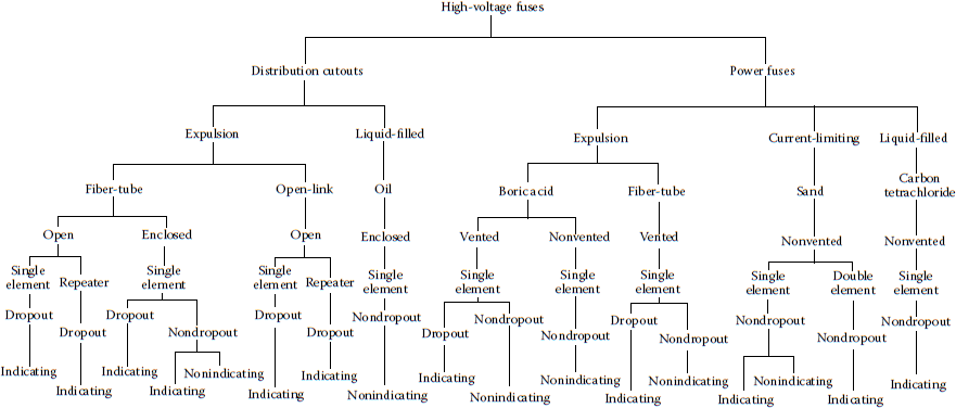
Classification of high-voltage fuses.
(From Westinghouse Electric Corporation, Electric Utility Engineering Reference Book-Distribution Systems. voi. 3, East Pittsburgh, PA, 1965.)
The liquid-filled (oil-filled) cutouts are mainly used in underground installations and contain the fusible elements in an oil-filled and sealed tank. The expulsion-type distribution cutouts are by far the most common type of protective device applied to overhead primary distribution systems. In these cutouts, the melting of the fuse link causes heating of the fiber fuse tube, which, in turn, produces deionizing gases to extinguish the arc.
Expulsion-type cutouts are classified according to their external appearance and operation methods as (1) enclosed-fuse cutouts, (2) open-fuse cutouts, and (3) open-link-fuse cutouts.
The ratings of the distribution fuse cutouts are based on continuous current-carrying capacity, nominal and maximum design voltages, and interrupting capacity. In general, the fuse cutouts are selected based upon the following data:
- The type of system for which they are selected, for example, overhead or underground and delta or grounded-wye system
- The system voltage for which they are selected
- The maximum available fault current at the point of application
- The X/R ratio at the point of application
- Other factors, for example, safety, load growth, and changing duty requirements
The use of symmetrical ratings simplified the selection of cutouts as a simple comparison of the calculated system requirements with the available fuse cutout ratings. In spite of that, fuse cutouts still have to be able to interrupt asymmetrical currents, which are, in turn, subject to the X/R ratios of the circuit. Therefore, symmetrical cutout rating tables are prepared on the basis of assumed maximum X/R ratios. Table 10.1 gives the interrupting ratings of open-fuse cutouts. Figure 10.2 shows a typical open-fuse cutout in pole-top style for 7.2/14.4 kV overhead distribution. Figure 10.3 shows a typical application of open-fuse cutouts in 7.2/14.4 kV overhead distribution.
Interrupting Ratings of Open-Fuse Cutouts
Rating of Cutout |
Interrupting Rating in Root-Mean-Rating of Cutout Square Amperes at |
||||||
|---|---|---|---|---|---|---|---|
Continuous |
Nominai |
Maximum Design |
Interrupting Rating Nomenclature |
||||
Current, A |
Voltage, kV |
Voltage, kV |
5.2 kV |
7.8 kV |
15 kV |
27 kV |
|
100 |
5.0 |
5.2 |
3,000 |
— |
— |
— |
Normal duty |
100 |
5.0 |
5.2 |
5,000 |
— |
— |
— |
Heavy duty |
100 |
5.0 |
5.2 |
10,000 |
— |
— |
— |
Extra heavy duty |
200 |
5.0 |
5.2 |
4,000 |
— |
— |
— |
Normal duty |
200 |
5.0 |
5.2 |
12,000 |
— |
— |
— |
Heavy duty |
100 |
7.5 |
7.8 |
— |
3,000 |
— |
— |
Normal duty |
100 |
7.5 |
7.8 |
— |
5,000 |
— |
— |
Heavy duty |
100 |
7.5 |
7.8 |
— |
10,000 |
— |
— |
Extra heavy duty |
200 |
7.5 |
7.8 |
— |
4,000 |
— |
— |
Normal duty |
200 |
7.5 |
7.8 |
— |
12,000 |
— |
— |
Heavy duty |
100 |
15 |
15 |
— |
— |
2,000 |
— |
Normal duty |
100 |
15 |
15 |
— |
— |
4,000 |
— |
Heavy duty |
100 |
15 |
15 |
— |
— |
8,000 |
— |
Extra heavy duty |
200 |
15 |
15 |
— |
— |
4,000 |
— |
Normal duty |
200 |
15 |
15 |
— |
— |
10,000 |
— |
Heavy duty |
100 |
25 |
27 |
— |
— |
— |
1200 |
Normal duty |
Source: Westinghouse Electric Corporation, Electric Utility Engineering Reference Book—Distribution Systems, vol. 3, East Pittsburgh, PA, 1965. With permission.

Typical application of open-fuse cutouts in 7.2/14.4 kV overhead distribution.
(Courtesy of S&C Electric Company, Chicago, IL.)

Typical application of open-fuse cutouts in 7.2/14.4 kV overhead distribution.
(Courtesy of S&C Electric Company, Chicago, IL.)
In 1951, a joint study by the Edison Electric Institute (EEI) and National Electrical Manufacturers Association (NEMA) established standards specifying preferred and nonpreferred current ratings for fuse links of distribution fuse cutouts and their associated TCCs in order to provide interchangeability for fuse links.
The reason for stating certain ratings to be preferred or nonpreferred is based on the fact that the ordering sequence of the current ratings is set up such that a preferred-size fuse link will protect the next higher preferred size. This is also true for the nonpreferred sizes. The current ratings of fuse links for preferred sizes are given as 6, 10, 15, 25, 40, 65, 100, 140, and 200 A and for nonpreferred sizes as 8, 12, 20, 30, 50, and 80 A.
Furthermore, the standards also classify the fuse links as (1) type K (fast) and (2) type T (slow). The difference between these two fuse links is in the relative melting time, which is defined by the speed ratio as
Speed ratio=Melting current at 0.1sMelting current at 300 or 600s
where
The 0.1 and 300 s are for fuse links rated 6–100 A
The 0.1 and 600 s are for fuse links rated 140–200 A
Therefore, the speed ratios for type K and type T fuse links are between 6 and 8, and 10 and 13, respectively. Figure 10.4 shows typical fuse links. Figure 10.5 shows minimum-melting TCC curves for typical (fast) fuse links.
Typical fuse links used on outdoor distribution: (a) fuse link rated less than 10 A and (b) fuse link rated 10-100 A.
(Courtesy of S&C Electric Company, Chicago, IL.)
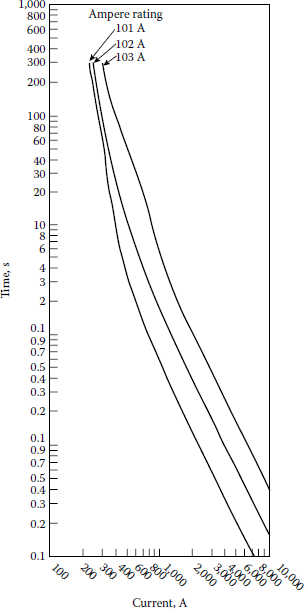
Minimum-melting-TCC curves for typical (fast) fuse links. Curves are plotted to minimum test points, so all variations should be +20% in current.
(Courtesy of S&C Electric Company, Chicago, IL.)
Power fuses are employed where the system voltage is 34.5 kV or higher and/or the interrupting requirements are greater than the available fuse cutout ratings. They are different from fuse cutouts in terms of (1) higher interrupting ratings, (2) larger range of continuous current ratings, (3) applicable not only for distribution but also for subtransmission and transmission systems, and (4) designed and built usually for substation mounting rather than pole and crossarm mounting. A power fuse is made of a fuse mounting and a fuse holder. Its fuse link is called the refill unit. In general, they are designed and built as (1) expulsion (boric acid or other solid material [SM]) type, (2) current-limiting (silver-sand) type, or (3) liquid-filled type.
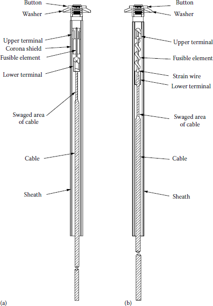
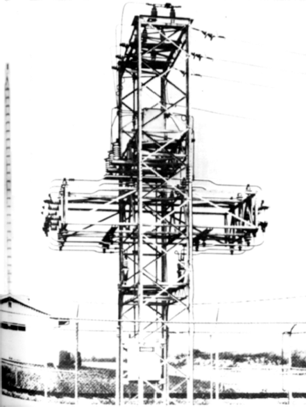
Power fuses are identified by the letter “E” (e.g., 200E or 300E) to specify that their TCCs comply with the interchangeability requirements of the standard. Figure 10.6 shows a typical transformer protection application of 34.5 kV SM-type power fuses. Figure 10.7 shows a feeder protection application of 34.5 kV SM-type power fuses. Figure 10.8 shows a cutaway view of a typical 34.5 kV SM-type refill unit.

Typical transformer protection application of 34.5 kV SM-type power fuses.
(Courtesy of S&C Electric Company, Chicago, IL.)
Feeder protection application of 34.5 kV SM-type power fuses.
(Courtesy of S&C Electric Company, Chicago, IL.)
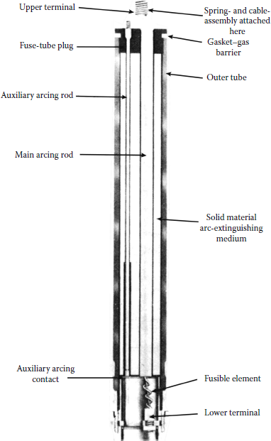
Cutaway view of typical 34.5 kV SM-type refill unit.
(Courtesy of S&C Electric Company, Chicago, IL.)
10.2.2 Automatic Circuit Reclosers
The automatic circuit recloser is an overcurrent protective device that automatically trips and recloses a preset number of times to clear temporary faults or isolate permanent faults. It also has provisions for manually opening and reclosing the circuit that is connected.
Reclosers can be set for a number of different operation sequences such as (1) two instantaneous (trip and reclose) operations followed by two time-delay trip operations prior to lockout, (2) one instantaneous plus three time-delay operations, (3) three instantaneous plus one timedelay operations, (4) four instantaneous operations, or (5) four time-delay operations. The instantaneous and time-delay characteristics of a recloser are a function of its rating. Recloser ratings range from 5 to 1120 A for the ones with series coils and from 100 to 2240 A for the ones with nonseries coils.
The minimum pickup for all ratings is usually set to trip instantaneously at two times the current rating. The reclosers must be able to interrupt asymmetrical fault currents related to their symmetrical rating. The root-mean-square (rms) asymmetrical current ratings can be determined by multiplying the symmetrical ratings by the asymmetrical factor, from Table 10.2, corresponding to the specified X/R circuit ratio. Note that the asymmetrical factors given in Table 10.2 are the ratios of the asymmetrical to the symmetrical rms fault currents at 0.5 cycle after fault initiation for different circuit X/R ratios.
Asymmetrical Factors as Function of X/R Ratios
X/R |
Asymmetrical Factor |
|---|---|
2 |
1.06 |
4 |
1.20 |
8 |
1.39 |
10 |
1.44 |
12 |
1.48 |
14 |
1.51 |
25 |
1.60 |
A generally accepted rule of thumb is to assume that the X/R ratios on distribution feeders are not to surpass 5 and therefore the corresponding asymmetry factor is to be about 1.25. However, the asymmetry factor for other parts of the system is assumed to be approximately 1.6.
Line reclosers are often installed at points on the circuit to reduce the amount of exposure on the substation equipment. For example, a feeder circuit serving both urban and rural load would probably have reclosers on the main line serving the rural load. Therefore, the installation of line reclosers will depend on the amount of exposure and operating experience. The maximum fault current available is always an important consideration in the application of line reclosers.
In a sense, a recloser fulfills the same task as the combination of a circuit breaker, overcurrent relay, and reclosing relay. Fundamentally, a recloser is made of an interrupting chamber and the related main contacts that operate in oil, a control mechanism to trigger tripping and reclosing, an operator integrator, and a lockout mechanism.
Reclosers are designed and built in either single-phase or three-phase units. Single-phase reclosers inherently result in better service reliability as compared to three-phase reclosers. If the threephase primary circuit is wye connected, either a three-phase recloser or three single-phase reclosers are used. However, if the three-phase primary circuit is delta connected, the use of two single-phase reclosers is adequate for protecting the circuit against either single- or three-phase faults. Figure 10.9 shows a typical single-phase hydraulically controlled automatic circuit recloser. Figures 10.10 and 10.11 show typical three-phase hydraulically controlled and electronically controlled automatic circuit reclosers, respectively. Single-phase reclosers inherently result in better service reliability as compared to three-phase reclosers.
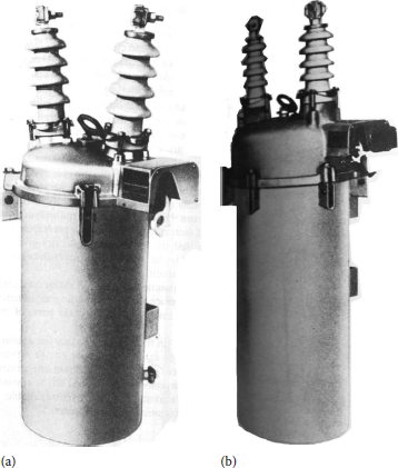
Typical single-phase hydraulically controlled automatic circuit recloser: (a) type H, 4H, V4H, or L and (b) type D, E, 4E, or DV.
(Courtesy of McGrawEdison Company, Belleville, NJ.)
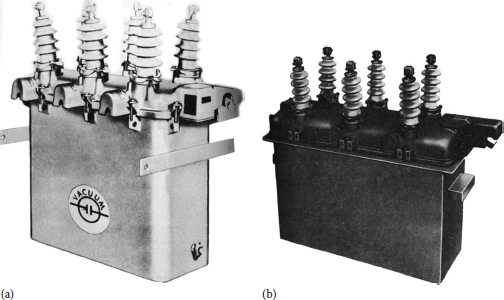
Typical three-phase hydraulically controlled automatic circuit reclosers: (a) type 6H or V6H and (b) type RV, RVE, RX, RXE, etc.
(Courtesy of McGraw-Edison Company, Belleville, NJ.)
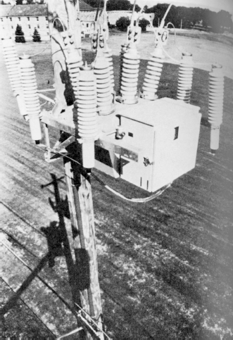
Typical three-pole automatic Circuit recloser.
(From Westinghouse Electric Corporation, Westinghouse Transmission and Distribution Reference Book, East Pittsburgh, PA, 1964; Westinghouse Electric Corporation, Electric Utility Engineering Reference Book-Distribution Systems, vol. 3, East Pittsburgh, PA, 1965.)
10.2.3 Automatic Line Sectionalizers
The automatic line sectionalizer is an overcurrent protective device installed only with backup circuit breakers or reclosers. It counts the number of interruptions caused by a backup automatic interrupting device and opens during dead circuit time after a preset number (usually two or three) of tripping operations of the backup device.
Zimmerman [1] summarizes the operation modes of a sectionalizer as follows:
- If the fault is cleared while the reclosing device is open, the sectionalizer counter will reset to its normal position after the circuit is reclosed.
- If the fault persists when the circuit is reclosed, the fault-current counter in the sectionalizer will again prepare to count the next opening of the reclosing device.
- If the reclosing device is set to go to lockout on the fourth trip operation, the sectionalizer will be set to trip during the open-circuit time following the third tripping operation of the reclosing device.
Contrary to expulsion-type fuses, a sectionalizer provides coordination (without inserting an additional time–current coordination) with the backup devices associated with very high fault currents and consequently provides an additional sectionalizing point on the circuit. On overhead distribution systems, they are usually installed on poles or crossarms. The application of sectionalizers entails certain requirements:
- They have to be used in series with other protective devices but not between two reclosers.
- The backup protective device has to be able to sense the minimum fault current at the end of the sectionalizer’s protective zone.
- The minimum fault current has to be greater than the minimum actuating current of the sectionalizer.
- Under no circumstances should the sectionalizer’s momentary and short-time ratings be exceeded.
- If there are two backup protective devices connected in series with each other and located ahead of a sectionalizer toward the source, the first and second backup devices should be set for four and three tripping operations, respectively, and the sectionalizer should be set to open during the second dead circuit time for a fault beyond the sectionalizer.
- If there are two sectionalizers connected in series with each other and located after a backup protective device that is close to the source, the backup device should be set to lockout after the fourth operation, and the first and second sectionalizers should be set to open following the third and second counting operations, respectively.
The standard continuous current ratings for the line sectionalizers range from 10 to 600 A. Figure 10.12 shows typical single- and three-phase automatic line sectionalizers.

Typical singleand three-phase automatic line sectionalizers: (a) type GH, (b) type GN3, (c) type GN3E, (d) type GV, (e) type GW, and (f) type GWC.
(Courtesy of McGraw-Edison Company, Belleville, NJ.)
The advantages of using automatic line sectionalizers are as follows:
- When employed as a substitute for reclosers, they have a lower initial cost and demand less maintenance.
- When employed as a substitute for fused cutouts, they do not show the possible coordination difficulties experienced with fused cutouts due to improperly sized replacement fuses.
- They may be employed for interrupting or switching loads within their ratings.
The disadvantages of using automatic line sectionalizers are as follows:
- When employed as a substitute for fused cutouts, they are more costly initially and demand more maintenance.
- In general, in the past, their failure rate has been greater than that of fused cutouts.
10.2.4 Automatic Circuit Breakers
Circuit breakers are automatic interrupting devices that are capable of breaking and reclosing a circuit under all conditions, that is, faulted or normal operating conditions. The primary task of a circuit breaker is to extinguish the arc that develops due to the separation of its contacts in an arcextinguishing medium, for example, in air, as is the case for air circuit breakers; in oil, as is the case for oil circuit breakers (OCBs); in SF6 (sulfur hexafluoride); or in vacuum. In some types, the arc is extinguished by a blast of compressed air, as is the case for magnetic blowout circuit breakers. The circuit breakers used at distribution system voltages are of the air circuit breaker or OCB type. For low-voltage applications, molded-case circuit breakers are available.
OCBs controlled by protective relays are usually installed at the source substations to provide protection against faults on distribution feeders.
Figures 10.13 and 10.14 show typical oil and vacuum circuit breakers, respectively.


Currently, circuit breakers are rated on the basis of rms symmetrical current. Usually, circuit breakers used in the distribution systems have minimum operating times of five cycles. In general, relay-controlled circuit breakers are preferred to reclosers due to their greater flexibility, accuracy, design margins, and esthetics. However, they are much more expensive than reclosers.
The relay, or fault-sensing device, that opens the circuit breaker is generally an overcurrent induction type with inverse, very inverse, or extremely inverse TCCs, for example, the CO relays by Westinghouse or the IAC relays by General Electric. Figure 10.15 shows a typical IAC single-phase overcurrent-relay unit. Figure 10.16 shows typical TCCs of overcurrent relays. Figure 10.17 shows time–current curves of typical overcurrent relays with inverse characteristics.

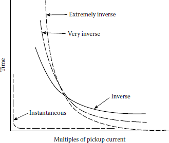
TCC of overcurrent relays.
(From General Electric Company, Distribution System Feeder Overcurrent Protection, Application Manual GET-6450, 1979.)
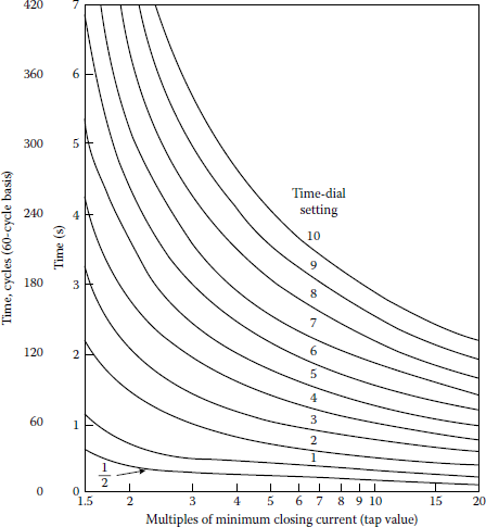
Time–current curves of IAC overcurrent relays with inverse characteristics.
(From General Electric Company, Overcurrent Protection for Distribution Systems, Application Manual GET-1751A, 1962; General Electric Company, Distribution System Feeder Overcurrent Protection, Application Manual GET6450, 1979.)
10.3 Objective of Distribution System Protection
The main objectives of distribution system protection are (1) to minimize the duration of a fault and (2) to minimize the number of consumers affected by the fault.
The secondary objectives of distribution system protection are (1) to eliminate safety hazards as fast as possible, (2) to limit service outages to the smallest possible segment of the system, (3) to protect the consumers’ apparatus, (4) to protect the system from unnecessary service interruptions and disturbances, and (5) to disconnect faulted lines, transformers, or other apparatus.
The overhead distribution systems are subject to two types of electric faults, namely, transient (or temporary) faults and permanent faults.
Depending on the nature of the system involved, approximately 75%-90% of the total number of faults are temporary in nature [2]. Usually, transient faults occur when phase conductors electrically contact other phase conductors or ground momentarily due to trees, birds or other animals, high winds, lightning, flashovers, etc. Transient faults are cleared by a service interruption of sufficient length of time to extinguish the power arc. Here, the fault duration is minimized, and unnecessary fuse blowing is prevented by using instantaneous or high-speed tripping and automatic reclosing of a relay-controlled power circuit breaker or the automatic tripping and reclosing of a circuit recloser. The breaker speed, relay settings, and recloser characteristics are selected in a manner to interrupt the fault current before a series fuse (i.e., the nearest source-side fuse) is blown, which would cause the transient fault to become permanent.
Permanent faults are those that require repairs by a repair crew in terms of (1) replacing burned-down conductors, blown fuses, or any other damaged apparatus; (2) removing tree limbs from the line; and (3) manually reclosing a circuit breaker or recloser to restore service. Here, the number of customers affected by a fault is minimized by properly selecting and locating the protective apparatus on the feeder main, at the tap point of each branch, and at critical locations on branch circuits.
Permanent faults on overhead distribution systems are usually sectionalized by means of fuses. For example, permanent faults are cleared by fuse cutouts installed at submain and lateral tap points. This practice limits the number of customers affected by a permanent fault and helps locate the fault point by reducing the area involved. In general, the only part of the distribution circuit not protected by fuses is the main feeder and feeder tie line. The substation is protected from faults on feeder and tie lines by circuit breakers and/or reclosers located inside the substation.
Most of the faults are permanent on an underground distribution system, thereby requiring a different protection approach. Even though the number of faults occurring on an underground system is relatively much less than that on the overhead systems, they are usually permanent and can affect a larger number of customers. Faults occurring in the underground residential distribution (URD) systems are cleared by the blowing of the nearest sectionalizing fuse or fuses. Faults occurring on the feeder are cleared by tripping and lockout of the feeder breaker.
Figure 10.18 shows a protection scheme of a distribution feeder circuit. As shown in the figure, each distribution transformer has a fuse that is located either externally, that is, in a fuse cutout next to the transformer, or internally, that is, inside the transformer tank as is the case for a completely self-protected (CSP) transformer.
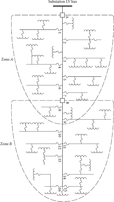
As shown in Figure 10.18, it is a common practice to install a fuse at the head of each lateral (or branch). The fuse must carry the expected load, and it must coordinate with load-side transformer fuses or other devices. It is customary to select the rating of each lateral fuse adequately large so that it is protected from damage by the transformer fuses on the lateral. Furthermore, the lateral fuse is usually expected to clear faults occurring at the ends of the lateral. If the fuse does not clear the faults, then one or more additional fuses may be installed on the lateral.
As shown in the figure, a recloser, or circuit breaker A with reclosing relays, is located at the substation to provide a backup protection. It clears the temporary faults in its protective zone. At the limit of the protective zone, the minimum available fault current, determined by calculation, is equal to the smallest value of current (called minimum pickup current), which will trigger the recloser, or circuit breaker, to operate. However, a fault beyond the limit of this protection zone may not trigger the recloser, or circuit breaker, to operate. Therefore, this situation may require that a second recloser, with a lower pickup current rating, be installed at location B, as shown in the figure.
The major factors that play a role in making a decision to choose a recloser over a circuit breaker are (1) the costs of equipment and installation and (2) the reliability. Usually, a comparable recloser can be installed for approximately one-third less than a relay-controlled OCB. Even though a circuit breaker provides a greater interrupting capability, this excess capacity is not always required. Also, some distribution engineers prefer reclosers because of their flexibility, due to the many extras that are available with reclosers but not with circuit breakers.
10.4 Coordination of Protective Devices
The process of selecting overcurrent protection devices with certain time–current settings and their appropriate arrangement in series along a distribution circuit in order to clear faults from the lines and apparatus according to a preset sequence of operation is known as coordination. When two protective apparatus installed in series have characteristics that provide a specified operating sequence, they are said to be coordinated or selective. Here, the device that is set to operate first to isolate the fault (or interrupt the fault current) is defined as the protecting device. It is usually the apparatus closer to the fault.
The apparatus that furnishes backup protection but operates only when the protecting device fails to operate to clear the fault is defined as the protected device. Properly coordinated protective devices help (1) to eliminate service interruptions due to temporary faults, (2) to minimize the extent of faults in order to reduce the number of customers affected, and (3) to locate the fault, thereby minimizing the duration of service outages.
Since coordination is primarily the selection of protective devices and their settings to develop zones that provide temporary fault protection and limit an outage area to the minimum size possible if a fault is permanent, to coordinate protective devices, in general, the distribution engineer must assemble the following data:
- Scaled feeder-circuit configuration diagram (map)
- Locations of the existing protective devices
- TCC curves of protective devices
- Load currents (under normal and emergency conditions)
- Fault currents or megavoltamperes (under minimum and maximum generation conditions) at every point where a protective apparatus might be located
Usually, these data are not readily available and therefore must be brought together from numerous sources. For example, the TCCs of protective devices are gathered from the manufacturers; the values of the load currents and fault currents are usually taken from computer runs called the load flow (or more correctly, power flow) studies and fault studies, respectively.
In general, manual techniques for coordination are still employed by most utilities, especially where distribution systems are relatively small or simple and therefore only a small number of protective devices are used in series.
However, some utilities have established standard procedures, tables, or other means to aid the distribution engineer and field personnel in coordination studies. Some utilities employ semiautomated, computerized coordination programs developed either by the protective device manufacturers or by the company’s own staff.
A general coordination procedure, regardless of whether it is manual or computerized, can be summarized as follows [3,4]:
- Gather the required and aforementioned data.
- Select initial locations on the given distribution circuit for protective (i.e., sectionalizing) devices.
- Determine the maximum and minimum values of fault currents (specifically for threephase, line-to-line [L–L], and line-to-ground faults) at each of the selected locations and at the end of the feeder mains, branches, and laterals.
- Pick out the necessary protective devices located at the distribution substation in order to protect the substation transformer properly from any fault that might occur in the distribution circuit.
- Coordinate the protective devices from the substation outward or from the end of the distribution circuit back to the substation.
- Reconsider and change, if necessary, the initial locations of the protective devices.
- Reexamine the chosen protective devices for current-carrying capacity, interrupting capacity, and minimum pickup rating.
- Draw a composite TCC curve showing the coordination of all protective devices employed, with curves drawn for a common base voltage (this step is optional).
- Draw a circuit diagram that shows the circuit configuration, the maximum and minimum values of the fault currents, and the ratings of the protective devices employed.
There are also some additional factors that need to be considered in the coordination of protective devices (i.e., fuses, reclosers, and relays) such as (1) the differences in the TCCs and related manufacturing tolerances, (2) preloading conditions of the apparatus, (3) ambient temperature, and (4) effect of reclosing cycles. These factors affect the adequate margin for selectivity under adverse conditions.
10.5 Fuse-To-Fuse Coordination
The selection of a fuse rating to provide adequate protection to the circuit beyond its location is based upon several factors. First of all, the selected fuse must be able to carry the expanded load current, and, at the same time, it must be sufficiently selective with other protective apparatus in series. Furthermore, it must have an adequate reach; that is, it must have the capability to clear a minimum fault current within its zone in a predetermined time duration.
A fuse is designed to blow within a specified time for a given value of fault current. The TCCs of a fuse are represented by two curves: the minimum-melting curve and the total-clearing curve, as shown in Figure 10.19. The minimum-melting curve of a fuse that represents the minimum time, and therefore it is the plot* of the minimum time versus current required to melt the fuse. The total-clearing (time) curve represents the total time, and therefore it is the plot of the maximum time versus current required to melt the fuse and extinguish the arc, plus manufacturing tolerance. It is also a standard procedure to develop “damaging” time curves from the minimum-melting-time curves by using a safety factor of 25%. Therefore, the damaging curve (due to the partial melting) is developed by taking 75% of the minimum-melting time of a specific-size fuse at various current values. The time unit used in these curves is seconds.

Fuse-to-fuse coordination, that is, the coordination between fuses connected in series, can be achieved by two methods:
- Using the TCC curves of the fuses
- Using the coordination tables prepared by the fuse manufacturers
Furthermore, some utilities employ certain rules of thumb as a third type of fuse-to-fuse coordination method.
In the first method, the coordination of the two fuses connected in series, as shown in Figure 10.19, is achieved by comparing the total-clearing-time–current curve of the “protecting fuse,” that is, fuse B, with the damaging-time curve of the “protected fuse,” that is, fuse A. Here, it is necessary that the total-clearing time of the protecting fuse not exceed 75% of the minimum-melting time of the protected fuse.
The 25% margin has been selected to take into account some of the operating variables, such as preloading, ambient temperature, and the partial melting of a fuse link due to a fault current of short duration. If there is no intersection between the aforementioned curves, a complete coordination in terms of selectivity is achieved. However, if there is an intersection of the two curves, the associated current value at the point of the intersection gives the coordination limit for the partial coordination achieved.
In the second method of fuse-to-fuse coordination, coordination is established by using the fuse sizes from coordination tables developed by the fuse link manufacturers. Tables 10.3 and 10.4 are such tables developed by the General Electric Company for fast and slow fuse links, respectively.
Coordination Table for GE Type "K" (Fast) Fuse Links Used in GE 50,100, or 200 A Expulsion Fuse Cutouts and Connected in Series
Type "K" Ratings of Protecting Fuse Links (B in Diagram), A |
Type "K" Ratings of Protected Fuse Links (A in Diagram), A |
||||||||||||||||||
|---|---|---|---|---|---|---|---|---|---|---|---|---|---|---|---|---|---|---|---|
6 K |
8 K |
10 K |
12 K |
15 K |
20 K |
25 K |
30 K |
40 K |
50 K |
65 K |
80 K |
52a |
100 K |
101a |
140 K |
200 K |
102a |
103a | |
Maximum short-cìrcuìt RMS Amperes to whichfuse links will be protected |
|||||||||||||||||||
1 K |
135 |
215 |
300 |
395 |
530 |
660 |
820 |
1100 |
1370 |
1720 |
2200 |
2750 |
3250 |
3600 |
5800 |
6000 |
9700 |
9500 |
16,000 |
2 K |
110 |
195 |
300 |
395 |
530 |
660 |
820 |
1100 |
1370 |
1720 |
2200 |
2750 |
3250 |
3600 |
5800 |
6000 |
9700 |
9500 |
16,000 |
3 K |
80 |
165 |
290 |
395 |
530 |
660 |
820 |
1100 |
1370 |
1720 |
2200 |
2750 |
3250 |
3600 |
5800 |
6000 |
9700 |
9500 |
16,000 |
5 A series hi-surge |
14 |
133 |
270 |
395 |
530 |
660 |
820 |
1100 |
1370 |
1720 |
2200 |
2750 |
3250 |
3600 |
5800 |
6000 |
9700 |
9500 |
16,000 |
6 K |
37 |
145 |
270 |
460 |
620 |
820 |
1100 |
1370 |
1720 |
2200 |
2750 |
3250 |
3600 |
5800 |
6000 |
9700 |
9500 |
16,000 | |
8 K |
133 |
170 |
390 |
560 |
820 |
1100 |
1370 |
1720 |
2200 |
2750 |
3250 |
3600 |
5800 |
6000 |
9700 |
9500 |
16,000 | ||
10 A series hi-surge |
16 |
24 |
260 |
530 |
660 |
820 |
1100 |
1370 |
1720 |
2200 |
2750 |
3250 |
3600 |
5800 |
6000 |
9700 |
9500 |
16,000 | |
10 K |
38 |
285 |
470 |
720 |
1100 |
1370 |
1720 |
2200 |
2750 |
3250 |
3600 |
5800 |
6000 |
9700 |
9500 |
16,000 | |||
12 K |
140 |
360 |
660 |
1100 |
1370 |
1720 |
2200 |
2750 |
3250 |
3600 |
5800 |
6000 |
9700 |
9500 |
16,000 | ||||
15 K |
95 |
410 |
960 |
1370 |
1720 |
2200 |
2750 |
3250 |
3600 |
5800 |
6000 |
9700 |
9500 |
16,000 | |||||
20 K |
70 |
700 |
1200 |
1720 |
2200 |
2750 |
3250 |
3600 |
5800 |
6000 |
9700 |
9500 |
16,000 | ||||||
25 K |
140 |
580 |
1300 |
2200 |
2750 |
3250 |
3600 |
5800 |
6000 |
9700 |
9500 |
16,000 | |||||||
30 K |
215 |
700 |
1800 |
2750 |
3250 |
3600 |
5800 |
6000 |
9700 |
9500 |
16,000 | ||||||||
40 K |
170 |
1200 |
2750 |
3250 |
3600 |
5800 |
6000 |
9700 |
9500 |
16,000 | |||||||||
50 K |
195 |
1600 |
3250 |
3600 |
5800 |
6000 |
9700 |
9500 |
16,000 | ||||||||||
65 K |
330 |
2300 |
5800 |
6000 |
9700 |
9500 |
16,000 | ||||||||||||
52a |
290 |
5500 |
6000 |
9700 |
9500 |
16,000 | |||||||||||||
80 K |
580 |
5800 |
6000 |
9700 |
9500 |
16,000 | |||||||||||||
100 K |
300 |
4300 |
9700 |
9500 |
16,000 | ||||||||||||||
101a |
385 |
7500 |
16,000 | ||||||||||||||||
140 K |
2800 |
16,000 | |||||||||||||||||
102a |
1250 |
||||||||||||||||||
Source: General Electric Company, Overcurrent Protection for Distribution Systems, Application Manual GET-1751 A, 1962. With permission. RMS, root-mean-square.
a GE coordinating fuse links.
Coordination Table for GE Type "T" (Slow) Fuse Links Used in GE 50,100, or 200 A Expulsion Fuse Cutouts and Connected in Series
Type "T" Ratings of Protected Fuse Links (B in Diagram), A |
Type "T" Ratings of Protected Fuse Links (A in Diagram), A |
|||||||||||||||
|---|---|---|---|---|---|---|---|---|---|---|---|---|---|---|---|---|
6T |
8T |
10T |
12T |
15T |
20T |
25T |
30T |
40T |
50T |
65 T |
80T |
100T |
140T |
200T |
103 |
|
Maximum short-circuit RMS Amperes to which fuse links will be protected |
||||||||||||||||
lNa |
250 |
395 |
540 |
710 |
950 |
1220 |
1500 |
1930 |
2500 |
3100 |
3950 |
4950 |
6300 |
9600 |
15,000 |
16,000 |
2Na |
250 |
395 |
540 |
710 |
950 |
1220 |
1500 |
1930 |
2500 |
3100 |
3950 |
4950 |
6300 |
9600 |
15,000 |
16,000 |
3Na |
250 |
395 |
540 |
710 |
950 |
1220 |
1500 |
1930 |
2500 |
3100 |
3950 |
4950 |
6300 |
9600 |
15,000 |
16,000 |
6T |
33 |
365 |
650 |
950 |
1220 |
1500 |
1930 |
2500 |
3100 |
3950 |
4950 |
6300 |
9600 |
15,000 |
16,000 |
|
8T |
125 |
480 |
850 |
1220 |
1500 |
1930 |
2500 |
3100 |
3950 |
4950 |
6300 |
9600 |
15,000 |
16,000 |
||
10 A series hi-surge |
19 |
540 |
710 |
950 |
1220 |
1500 |
1930 |
2500 |
3100 |
3950 |
4950 |
6300 |
9600 |
15,000 |
16,000 |
|
10T |
74 |
620 |
1130 |
1500 |
1930 |
2500 |
3100 |
3950 |
4950 |
6300 |
9600 |
15,000 |
16,000 |
|||
12T |
135 |
770 |
1400 |
1930 |
2500 |
3100 |
3950 |
4950 |
6300 |
9600 |
15,000 |
16,000 |
||||
15T |
100 |
880 |
1750 |
2500 |
3100 |
3950 |
4950 |
6300 |
9600 |
15,000 |
16,000 |
|||||
20T |
105 |
1150 |
2300 |
3100 |
3950 |
4950 |
6300 |
9600 |
15,000 |
16,000 |
||||||
25T |
190 |
1500 |
3100 |
3950 |
4950 |
6300 |
9600 |
15,000 |
16,000 |
|||||||
30T |
115 |
1900 |
3950 |
4950 |
6300 |
9600 |
15,000 |
16,000 |
||||||||
40T |
310 |
2350 |
4950 |
6300 |
9600 |
15000 |
16,000 |
|||||||||
50T |
150 |
3400 |
6300 |
9600 |
15000 |
16,000 |
||||||||||
65T |
270 |
4300 |
9600 |
15000 |
16,000 |
|||||||||||
80T |
660 |
9200 |
15,000 |
16,000 |
||||||||||||
100T |
6000 |
15,000 |
16,000 |
|||||||||||||
140T |
6600 |
|||||||||||||||
RMS, root-mean-square.
a The IN, 2N, and 3N ampere ratings of the GE 5 A series hi-surge fuse links have TCCs closely approaching those established by the American Standards for IT, 2T, and 3T ampere ratings, respectively. Hence, they are recommended for applications requiring IT, 2T, or 3T fuse links.
These tables give the maximum fault currents to achieve coordination between various fuse sizes and are based upon the 25% margin described in the first method. Here, the determination of the total-clearing curve is not necessary since the maximum value of fault current to which each combination of series fuses can be subjected with guaranteed coordination is given in the tables, depending upon the type of fuse link selected.
10.6 Recloser-To-Recloser Coordination
The need for recloser-to-recloser coordination may arise due to any of the following situations that may exist in a given distribution system:
- Having two three-phase reclosers
- Having two single-phase reclosers
- Having a three-phase recloser at the substation and a single-phase recloser on one of the branches of a given feeder
The required coordination between the reclosers can be achieved by using one of the following remedies:
- Employing different recloser types and some mixture of coil sizes and operating sequences
- Employing the same recloser type and operating sequence but using different coil sizes
- Employing the same recloser type and coil sizes but using different operating sequences
In general, the utility industry prefers to use the first remedy over the other two. However, there may be some circumstances, for example, having two single-phase reclosers of the same type, where the second remedy can be applied.
When the TCC curves of the two reclosers are less than 12 cycles separate from each other, the reclosers may do their instantaneous or fast operations at the same time. To achieve coordination between the delayed-tripping curves of two reclosers, at least a minimum time margin of 25% must be applied.
10.7 Recloser-To-Fuse Coordination
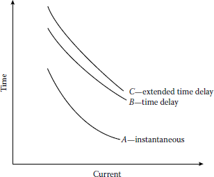
In Figure 10.20, curves represent the instantaneous, time-delay, and extended time-delay (as an alternative) tripping characteristics of a conventional automatic circuit recloser. Here, curves A and B symbolize the first and second openings and the third and fourth openings of the recloser, respectively.
To provide protection against permanent faults, fuse cutouts (or power fuses) are installed on overhead feeder taps and laterals. The use of an automatic reclosing device as a backup protection against temporary faults eliminates many unnecessary outages that occur when using fuses only. Here, the backup recloser can be either the substation feeder recloser, usually with an operating sequence of one fast- and two delayed-tripping operations, or a branch feeder recloser, with two fast- and two delayed-tripping operations. The recloser is set to trip for a temporary fault before any of the fuses can blow and then reclose the circuit. However, if the fault is a permanent one, it is cleared by the correct fuse before the recloser can go on time-delay operation following one or two instantaneous operations.
Figure 10.21 shows a portion of a distribution system where a recloser is installed ahead of a fuse. The figure also shows the superposition of the TCC curve of the fuse C on the fast and delayed TCC curves of the recloser R. If the fault beyond fuse C is temporary, the instantaneous tripping operations of the recloser protect the fuse from any damage. This can be observed from the figure by the fact that the instantaneous recloser curve A lies below the fuse TCC for currents less than that associated with the intersection point b.
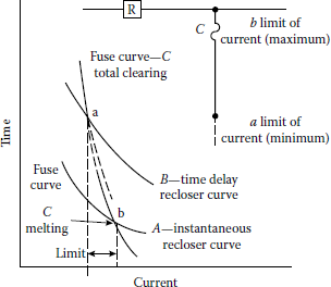
Recloser TCC curves superimposed on fuse TCC curves.
(From General Electric Company, Distribution System Feeder Overcurrent Protection, Application Manual GET-6450, 1979.)
However, if the fault beyond fuse C is a permanent one, the fuse clears the fault as the recloser goes through a delayed operation B. This can be observed from the figure by the fact that the timedelay curve B of the recloser lies above the total-clearing-curve portion of the fuse TCC for currents greater than that associated with the intersection point a. The distance between the intersection points a and b gives the coordination range for the fuse and recloser.
Therefore, a proper coordination of the trip operations of the recloser and the total-clearing time of the fuse prevents the fuse link from being damaged during instantaneous trip operations of the recloser. The required coordination between the recloser and the fuse can be achieved by comparing the respective time–current curves and taking into account other factors, for example, preloading, ambient temperature, curve tolerances, and accumulated heating and cooling of the fuse link during the fast-trip operations of the recloser.
Figure 10.22 illustrates the temperature cycle of a fuse link during recloser operations. As can be observed from the figure, each of the first two (instantaneous) operations takes only 2 cycles, but each of the last two (delayed) operations lasts 20 cycles. After the fourth operation, the recloser locks itself open.

Temperature cycle of fuse link during recloser operation.
(From General Electric Company, Distribution System Feeder Overcurrent Protection, Application Manual GET-6450, 1979.)
Therefore, the recloser-to-fuse coordination method illustrated in Figure 10.21 is an approximate one since it does not take into account the effect of the accumulated heating and cooling of the fuse link during recloser operation. Thus, it becomes necessary to compute the heat input to the fuse during, for example, two instantaneous recloser operations if the fuse is to be protected from melting during these two openings.
Figure 10.23 illustrates a practical yet sufficiently accurate method of coordination. Here, the maximum coordinating current is found by the intersection (at point b') of two curves, the fusedamage curve (which is defined as 75% of the minimum-melting-time curve of the fuse) and the maximum-clearing-time curve of the recloser’s fast-trip operation (which is equal to 2 × A “in time,” since there are two fast trips). Similarly, point a' is found from the intersection of the fuse totalclearing curve with the shifted curve B' (which is equal to 2 × A + 2 × B “in time,” since in addition to the two fast trips, there are two delayed trips).
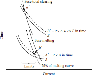
Recloser-to-fuse coordination (corrected for heating and cooling cycle).
(From General Electric Company, Distribution System Feeder Overcurrent Protection, Application Manual GET-6450, 1979.)
Some distribution engineers use rule-of-thumb methods, based upon experience, to allow extra margin in the coordination scheme.
As shown in Table 10.5, there are also coordination tables developed by the manufacturers to coordinate reclosers with fuse links in a simpler way.
Automatic Recloser and Fuse Ratings
Recloser Rating, rms A (Continuos) |
Fuse Link Rating, rma A |
2Na |
3Na |
Ratings of GE Type T Fuse Links, A |
||||||
|---|---|---|---|---|---|---|---|---|---|---|
6T |
8T |
10T |
12T |
15T |
20T |
25T |
||||
Range of Coordination, rms A |
||||||||||
5 |
Min |
14 |
17.5 |
68 |
||||||
Max |
55 |
55 |
123 |
|||||||
10 |
Min |
31 |
45 |
75 |
200 |
|||||
Maxb |
110 |
152 |
220 |
300, 250 |
||||||
15 |
Min |
30 |
34 |
59 |
84 |
200 |
380 |
|||
Maxb |
105 |
145 |
210 |
280 |
375 |
450c |
||||
25 |
Min |
50 |
50 |
50 |
68 |
105 |
145 |
300 |
||
Max |
89 |
130 |
190 |
265 |
360 |
480 |
610 |
|||
Source: Fink, D.G. and H.W. Beaty, Standard Handbook for Electrical Engineers, 11th edn., McGraw-Hill, New York, 1978. With permission.
a The 1N, 2N, and 3N ampere ratings of the GE 5 A series hi-surge fuse links have TCCs closely approaching those established by the EEI-NEMA Standards for IT, 2T, and 3T ampere ratings, respectively. Hence, they are recommended for applications requiring 1T, 2T, or 3T fuse links.
b Where maximum lines have two values, the smaller value is for the 50 A frame, single-phase recloser. The larger value is for all others: 50 A frame, three phase; 140 A frame, single phase and three phase.
c Coordination with 50 A frame size single-phase recloser not possible since maximum interrupting capacity is less than minimum value.
10.8 Recloser-To-Substation Transformer High-Side Fuse Coordination
Usually, a power fuse, located at the primary side of a delta–wye-connected substation transformer, provides protection for the transformer against the faults in the transformer or at the transformer terminals and also provides backup protection for feeder faults. These fuses have to be coordinated with the reclosers or reclosing circuit breakers located on the secondary side of the transformer to prevent the fuse from any damage during the sequential tripping operations. The effects of the accumulated heating and cooling of the fuse element can be taken into account by adjusting the delayed-tripping time of the recloser.
To achieve a coordination, the adjusted tripping time is compared to the minimum-melting time of the fuse element, which is plotted for a phase-to-phase fault that might occur on the secondary side of the transformer. If the minimum-melting time of the backup fuse is greater than the adjusted tripping time of the recloser, a coordination between the fuse and recloser is achieved.
The coordination of a substation circuit breaker with substation transformer primary fuses dictates that the total-clearing time of the circuit breaker (i.e., relay time plus breaker interrupting time) be less than 75%–90% of the minimum-melting time of the fuses at all values of current up to the maximum fault current.
The selected fuse must be able to carry 200% of the transformer full-load current continuously in any emergency in order to be able to carry the transformer “magnetizing” inrush current (which is usually 12–15 times the transformer full-load current) for 0.1 s [5].
10.9 Fuse-To-Circuit-Breaker Coordination
The fuse-to-circuit-breaker (overcurrent-relay) coordination is somewhat similar to the fuse-torecloser coordination. In general, the reclosing time intervals of a circuit breaker are greater than those of a recloser. For example, 5 s is usually the minimum reclosing time interval for a circuit breaker, whereas the minimum reclosing time interval for a recloser can be as small as 1/2 s.
Therefore, when a fuse is used as the backup or protected device, there is no need for heating and cooling adjustments. Thus, in order to achieve a coordination between a fuse and circuit breaker, the minimum-melting-time curve of the fuse is plotted for a phase-to-phase fault on the secondary side.
If the minimum-melting time of the fuse is approximately 135% of the combined time of the circuit breaker and related relays, the coordination is achieved. However, when the fuse is used as the protecting device, the coordination is achieved if the relay operating time is 150% of the totalclearing time of the fuse.
In summary, when the circuit breaker is tripped instantaneously, it has to clear the fault before the fuse is blown. However, the fuse has to clear the fault before the circuit breaker trips on timedelay operations.
Therefore, it is necessary that the relay characteristic curve, at all values of current up to the maximum current available at the fuse location, lie above the total-clearing characteristic curve of the fuse. Thus, it is usually customary to leave a margin between the relay and fuse characteristic curves to include a safety factor of 0.1 to 0.3 + 0.1 s for relay overtravel time.
A sectionalizing fuse installed at the riser pole to protect underground cables does not have to coordinate with the instantaneous trips since underground lines are usually not subject to transient faults. On looped circuits, the fuse size selected is usually the minimum size required to serve the entire load of the loop, whereas on lateral circuits, the fuse size selected is usually the minimum size required to serve the load and coordinate with the transformer fuses, keeping in mind the cold pickup load.
10.10 Recloser-To-Circuit-Breaker Coordination
The reclosing relay recloses its associated feeder-circuit breaker at predetermined intervals (e.g., 15, 30, or 45 s cycles) after the breaker has been tripped by overcurrent relays. If desired, the reclosing relay can provide an instantaneous initial reclosure plus three time-delay reclosures.
However, if the fault is permanent, the reclosing relay recloses the breaker the predetermined number of times and then goes to the lockout position. Usually, the initial reclosing is so fast that customers may not even realize that service has been interrupted.
The crucial factor in coordinating the operation of a recloser and a circuit breaker (better yet, the relay that trips the breaker) is the reset time of the overcurrent relays during the tripping and reclosing sequence.
If the relay used is of an electromechanical type, rather than a solid-state type, it starts to travel in the trip direction during the operation of the recloser.
If the reset time of the relay is not adjusted properly, the relay can accumulate enough movement (or travel) in the trip direction, during successive recloser operations, to trigger a false tripping.
Example 10.1
Figure 10.24 gives an example* for proper recloser-to-relay coordination. In the figure, curves A and B represent, respectively, the instantaneous and time-delay TCCs of the 35 A reclosers. Curve C represents the TCC of the extremely inverse-type IAC overcurrent relay set on the number 1.0 time-dial adjustment and 4 A tap (160 A primary with 200:5 current transformer [CT]). Assume a permanent fault current of 700 A located at point X in the figure. Determine the necessary relay and recloser coordination.

An example of recloser-to-relay coordination. Curve A represents TCCs of one instantaneous recloser opening. Curve B represents TCCs of one extended time-delay recloser opening. Curve C represents TCCs of the IAC relay.
(Courtesy of Sec Company, Chicago, IL.)
Solution
From Figure 10.24, the operating time of the relay and recloser can be found as the following:
For recloser: Instantaneous (from curve A) = 0.03 s
Time delay (from curve B) = 0.17 s
For relay: Pickup (from curve C) = 0.42 s
Reset=1.010×60−6.0s
assuming a 60 s reset time for the relay with a number 10 time-dial setting [5].
Using the signs (+) for trip direction and (−) for reset direction, the percent of total relay travel, during the operation of the recloser, can be calculated in the following manner. During the instantaneous operation (from curve A) of the recloser,
Relay-closing travel=Recloser-instantaneous timeRelay-pickup time=0.030.42=0.0714 or 7.14%(10.1)
Assuming that the recloser is open for 1 s,
Relay-reset travel=(−)Recloser-open timeRelay-reset time=−16.0=−0.1667 or −16.67%(10.2)
From the results, it can be seen that
|Relay-closing travel| < |relay-reset travel|
or
|7.14%| < |16.67%|
and therefore the relay will completely reset during the time that the recloser is open following each instantaneous opening.
Similarly, the travel percentages during the delayed-tripping operations can be calculated in the following manner. During the first time-delay trip operation (from curve B) of the recloser,
Relay-closing travel=Recloser time-delayRecloser-pickup time=0.170.42≅0.405 or −40.5%(10.3)
Assuming that the recloser opens for 1 s,
Relay-reset travel=(−)Recloser-open timeRelay-reset time=−1.06.0=−16.67%
During the second time-delay trip of the recloser,
Relay-closing travel = 40.5%
Therefore, the net total relay travel is 64.3%:
( = +40.5%−16.67%+ 40.5%)
Since this net total relay travel is less than 100%, the desired recloser-to-relay coordination is accomplished. In general, a 0.15–0.20 s safety margin is considered to be adequate for any possible errors that might be involved in terms of curve readings, etc.
Some distribution engineers use a rule-of-thumb method to determine whether the recloser-torelay coordination is achieved or not. For example, if the operating time of the relay at any given fault-current value is less than twice the delayed-tripping time of the recloser, assuming a recloser operation sequence that includes two time-delay trips, there will be a possible lack of coordination. Whenever there is a lack of coordination, either the time-dial or pickup settings of the relay must be increased or the recloser has to be relocated until the coordination is achieved.
In general, the reclosers are located at the end of the relay reach. The rating of each recloser must be such that it will carry the load current, have sufficient interrupting capacity for that location, and coordinate with both the relay and load-side apparatus. If there is a lack of coordination with the load-side apparatus, then the recloser rating has to be increased. After the proper recloser ratings are determined, each recloser has to be checked for reach. If the reach is insufficient, additional series reclosers may be installed on the primary main.
10.11 Fault-Current Calculations*
There are four possible fault types that might occur in a given distribution system:
- Three-phase grounded or ungrounded fault (3ϕ)
- Phase-to-phase (or L–L) ungrounded fault
- Phase-to-phase (or double line-to-ground, 2LG) grounded fault
- Phase-to-ground (or single line-to-ground, SLG) fault
The first type of fault can take place only on three-phase circuits, and the second and third on three-phase or two-phase (i.e., vee or open-delta) circuits. However, even on these circuits usually only SLG faults will take place due to the multigrounded construction. The relative numbers of the occurrences of different fault types depend upon various factors, for example, circuit configuration, the height of ground wires, voltage class, method of grounding, relative insulation levels to ground and between phases, speed of fault clearing, number of stormy days per year, and atmospheric conditions. Based on Ref. [6], the probabilities of prevalence of the various types of faults are†
SLG faults |
= 0.70 |
L-L faults |
= 0.15 |
2LG faults |
= 0.10 |
3ϕ faults |
= 0.05 |
Total |
= 1.00 |
The actual fault current is usually less than the bolted three-phase value. (Here, the term bolted means that there is no fault impedance [or fault resistance] resulting from fault arc, i.e., Zf = 0.) However, the SLG fault often produces a greater fault current that the 3ϕ fault especially (1) where the associated generators have solidly grounded neutrals or low-impedance neutral impedances and (2) on the wye-grounded side of delta–wye-grounded transformer banks [7].
Therefore, for a given system, each fault at each fault location must be calculated based on actual circuit conditions. When this is done, according to Anderson [8], it is usually the case that the SLG fault is the most severe, with the 3ϕ, 2LG, and L–L following in that order. In general, since the 2LG fault value is always somewhere in between the maximum and minimum, it is usually neglected in the distribution system fault calculations [3].
In general, the maximum and minimum fault currents are both calculated for a given distribution system. The maximum fault current is calculated based on the following assumptions:
- All generators are connected, that is, in service.
- The fault is a bolted one; that is, the fault impedance is zero.
- The load is maximum, that is, on-peak load.
The minimum current is calculated based on the following assumptions:
- The number of generators connected is minimum.
- The fault is not a bolted one, that is, the fault impedance is not zero but has a value somewhere between 0 and 40 Ω.
- The load is minimum, that is, off-peak load.
On 4 kV systems, the value of the minimum fault current available may be taken as 60%–70% of the calculated maximum line-to-ground fault current.
In general, these fault currents are calculated for each sectionalizing point, including the substation, and for the ends of the longest sections. The calculated maximum fault-current values are used in determining the required interrupting capacities (i.e., ratings) of the fuses, circuit breakers, or other fault-clearing apparatus; the calculated minimum fault-current values are used in coordinating the operations of fuses, reclosers, and relays.
To calculate the fault currents, one has to determine the zero-, positive-, and negative-sequence Thévenin impedances of the system* at the high-voltage side of the distribution substation transformer looking into the system. These impedances are usually readily available from transmission system fault studies. Therefore, for any given fault on a radial distribution circuit, one can simply add the appropriate impedances to the Thévenin impedances as the fault is moved away from the substation along the circuit. The most common types of distribution substation transformer connections are (1) delta–wye solidly grounded and (2) delta–delta.
10.11.1 Three-Phase Faults
Since this fault type is completely balanced, there are no zero- or negative-sequence currents. Therefore, when there is no fault impedance,
If,3ϕ=If,a=If,b=If,c=|ˉVL−NˉZ1|(10.4)
and when there is a fault impedance,
If,3ϕ=|ˉVL−NˉZ1+ˉZf|(10.5)
where
ˉIf,3ϕ is the three-phase fault current, A
ˉVL−N is the line-to-neutral distribution voltage, V
ˉZ1 is the total positive-sequence impedance, Ω
ˉZf is the fault impedance, Ω
If,3ϕ = If,a = If,b = If,c are the fault currents in a, b, and c phases
Since the total positive-sequence impedance can be expressed as
ˉZ1=ˉZ1,sys+ˉZ1,T+ˉZ1,ckt(10.6)
where
ˉZ1,sys is the positive-sequence Thévenin-equivalent impedance of the System (or source) referred to distribution voltage,* Ω
ˉZ1,T is the positive-sequence transformer impedance referred to distribution voltage,† Ω
ˉZ1,ckt is the positive-sequence impedance of faulted segment of distribution circuit, Ω
substituting Equation 10.6 into Equations 10.4 and 10.5, the three-phase fault current can be expressed as
If,3ϕ|ˉVL−NˉZ1,sys+ˉZ1,T+ˉZ1,ckt|A(10.7)
If,3ϕ|ˉVL−NˉZ1,sys+ˉZ1,T+ˉZ1,ckt+ˉZf|A(10.8)
Equations 10.7 and 10.8 are applicable whether the source connection is wye grounded or delta. At times, it might be necessary to reflect a three-phase fault on the distribution system as a threephase fault on the subtransmission system. This can be accomplished by using
IF3ϕ=VL−LVST,L−L×If3ϕA(10.9)
where
IF,3ϕ is the three-phase fault current referred to subtransmission voltage, A
If,3ϕ is the three-phase fault current based on distribution voltage, A
VL-L is the line-to-line distribution voltage, V
VST,L-L is the line-to-line subtransmission voltage, V
10.11.2 Line-To-Line Faults
Assume that an L–L fault exists between phases b and c. Therefore, if there is no fault impedance,
If,a=0If,L−L=If,c=−If,b=|j√3×ˉVL−NˉZ1+ˉZ2|(10.10)
where
If,L-L is the line-to-line fault current, A
ˉZ2 is the total negative-sequence impedance, Ω
However,
ˉZ1=ˉZ2
thus,
If,L−L=|j√3×ˉVL−N2ˉZ1|(10.11)
or substituting Equation 10.6 into Equation 10.11,
If,L−L=|j√3×ˉVL−N2(ˉZ1,sys+ˉZ1,T+ˉZ1,ckt)|(10.12)
However, if there is a fault impedance,
If,L−L=|j√3×ˉVL−N2(ˉZ1,sys+ˉZ1,T+ˉZ1,ckt)+ˉZf|(10.13)
By comparing Equation 10.11 with Equation 10.5, one can determine a relationship between the three-phase fault and L–L fault currents as
If,L−L=√32×If,3ϕ=0.866×If,3ϕ(10.14)
that is applicable to any point on the distribution system. The equations derived in this section are applicable whether the source connection is wye grounded or delta.
10.11.3 Single Line-To-Ground Faults
Assume that an SLG fault exists on phase a. If there is no fault impedance,
If,L−G=|ˉVL−NˉZG|(10.15)
where
If,L-G is the line-to-ground fault current, A
ˉZG is the impedance to ground, Ω
ˉVL−N is the line-to-neutral distribution voltage, V
ˉZG=ˉZ1+ˉZ2+ˉZ03(10.16)
However,
ˉZG=2ˉZ1+ˉZ03(10.17)
or
ˉZG=2ˉZ1+ˉZ03(10.17)
since
ˉZ1=ˉZ2
Therefore, by substituting Equation 10.17 into Equation 10.15,
If,L−G=|ˉVL−N13(2ˉZ1+ˉZ0)|(10.18)
However, if there is a fault impedance,
If,L−G=|ˉVL−N13(2ˉZ1+ˉZ0)+ˉZf|(10.19)
where ˉZ0 is the total zero-sequence impedance, Ω.
Equations 10.18 and 10.19 are only applicable if the source connection is wye grounded. If the source connection is delta, they are not applicable since the fault current would be equal to zero due to the zero-sequence impedance being infinite.
If the primary distribution feeders are supplied by a delta–wye solidly grounded substation transformer, an SLG fault on the distribution system is reflected as an L-L fault on the subtransmission system. Therefore, the low-voltage-side fault current may be referred to the high-voltage side by using the equation
If,L−L=VL−L√3×VST,L−L×If,L−G(10.20)
where
If,L-G is the single line-to-ground fault current based on distribution voltage, A
IF,L-L is the single line-to-ground fault current reflected as a line-to-line fault current on the subtransmission system, A
VL-L is the line-to-line distribution voltage, V
VST,L-L is the line-to-line subtransmission voltage, V
In general, the zero-sequence impedance Z0 of a distribution circuit with multigrounded neutral is very hard to determine precisely, but it is usually larger than its positive-sequence impedance Z1. However, some empirical approaches are possible. For example, Anderson [3] gives the following relationship between the zero- and positive-sequence impedances of a distribution circuit with multigrounded neutral:
ˉZ0=K0×ˉZ1(10.21)
where
Z0 is the zero-sequence impedance of distribution circuit, Ω
Z1 is the positive-sequence impedance of distribution circuit, Ω
K0 is a constant
Table 10.6 gives various possible values for the constant K0. If the earth has a very bad conducting characteristic, the constant K0 is totally established by the neutral-wire impedance. Anderson [3] suggests using an average value of 4 where exact conditions are not known.
Estimated Values of the K0 Constant for Various Conditions
Condition |
K0 |
|---|---|
Perfectly conducting earth (e.g., a system with multiple water-pipe grounds) |
1.0 |
Ground wire same size as phase wire |
4.0 |
Ground wire one size smaller |
4.6 |
Ground wire two sizes smaller |
4.9 |
Finite earth impedance |
3.8–4.2 |
Source: Anderson, P.M., Elements of Power System Protection, Cyclone Copy Center, Ames, IA, 1975.
10.11.4 Components of the Associated Impedance to the Fault
Impedance of the source: If the associated fault duty S given in megavoltamperes at the substation bus is available from transmission system fault studies, the system impedance, that is, “backup” impedance, can be calculated as
Z1,sys=VL−NIL=VL−L√3×IL(10.22)
but
IL=S√3×VL−L(10.23)
therefore
Z1,sys=V2L−LS(10.24)
If the system impedance is given at the transmission substation bus rather than at the distribution substation bus, then the subtransmission line impedance has to be involved in the calculations so that the total impedance (i.e., the sum of the system impedance and the subtransmission line impedance) represents the impedance up to the high side of the distribution substation transformer.
If the maximum three-phase fault current on the high-voltage side of the distribution substation transformer is known, then
Z1,sys+Z1,ST=VST,L−L√3(IF,3ϕ)max(10.25)
where
Z1,sys is the positive-sequence impedance of system, Ω
Z1,ST is the positive-sequence impedance of subtransmission line, Ω
VST,L-L is the line-to-line subtransmission voltage, V
(IF,3¢)max is the maximum three-phase fault current referred to subtransmission voltage, A
Note that the impedances found from Equation 10.24 and 10.25 can be referred to the base voltage by using Equation 10.9).
Impedance of the substation transformer: If the percent impedance of the substation transformer is known, the transformer impedance* can be expressed as
Z1,T=(%ZT)(V2L−L)10ST,3ϕ(10.26)
where
% ZT is the percent transformer impedance
VL-L is the line-to-line base voltage, kV
ST,3¢ is the three-phase transformer rating, kVA
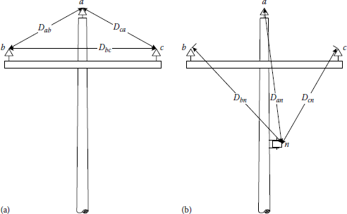
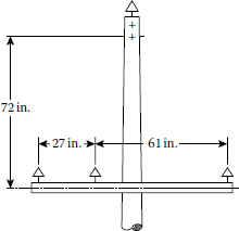
Impedance of the distribution circuits: The impedance values for the distribution circuits depend on the pole-top conductor configurations and can be calculated by means of symmetrical components. For example, Figure 10.25 shows a typical pole-top overhead distribution circuit configuration. The equivalent spacing (i.e., mutual geometric mean distance) of phase wires and the equivalent spacing between phase wires and neutral wire can be determined from
dp=Deq=DmΔ= (Dab×Dbc×Dca)1/3(10.27)
and
dnΔ= (Dan×Dbn×Dcn)1/3(10.28)
Similarly, the mutual reactances (spacing factors) for phase wires, and between phase wires and neutral wire (due to equivalent spacings), can be determined as
xdp=0.05292log10dp Ω/1000 ft(10.29)
and
- If the distribution circuit is a three-phase circuit,
The positive- and negative-sequence impedances are
and the zero-sequence impedance is
with
where
re is the resistance of earth = 0.0542 Ω/1000 ft
xe is the reactance of earth = 0.4676 Ω/1000 ft
xdn is the spacing factor between phase wires and neutral wire, Ω/1000 ft
xdp is the spacing factor for phase wires, Ω/1000 ft
rap is the resistance of phase wires, Ω/1000 ft
ran is the resistance of neutral wires, Ω/1000 ft
xap is the reactance of phase wire with 1 ft spacing, Ω/1000 ft
xan is the reactance of neutral wire with 1 ft spacing, Ω/1000 ft
z0,a is the zero-sequence self-impedance of phase circuit, Ω/1000 ft
z0,a is the zero-sequence self-impedance of one ground wire, Ω/1000 ft
z0,ag is the zero-sequence mutual impedance between the phase circuit as one group of conductors and the ground wire as other conductor group, Ω/1000 ft
- If the distribution circuit is an open-wye and single-phase delta circuit,
The positive- and negative-sequence impedances are
and the zero-sequence impedance is
where
- If the distribution circuit is a single-phase multigrounded circuit, Its impedance is
where
10.11.5 Sequence-Impedance Tables for the Application of Symmetrical Components
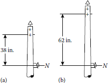
The zero-sequence-impedance equation (given as Equations 10.32, 10.37, or 10.41 in Section 10.11.4), that is,
can be expressed as or where
or
is the zero-sequence self-impedance of phase circuit, Ω/1000 ft
is the equivalent zero-sequence impedance due to combined effects of zero-sequence selfimpedance of one ground wire and zero-sequence mutual impedance between the phase circuit as one group of conductors and the ground wire as another conductor group, assuming a specific vertical distance between the ground wire and phase wires, for example, 38 in.
is the same as except the vertical distance is a different one, for example, 62 in.
Therefore, it is possible to develop precalculated sequence-impedance tables for the application of symmetrical components. For example, Figures 10.26 through 10.30 show various overhead pole-top conductor configurations with and without ground wire. The corresponding sequence-impedance values at 60 Hz and 50°C are given in Tables 10.7 through 10.11.
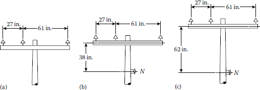
Various overhead pole-top conductor configurations: (a) without ground wire, (b) with ground wire, and (c) with ground wire, .

Various overhead pole-top conductor configurations: (a) without ground wire, z0 = z0,a, and (b) with ground wire, , and (c) with ground wire, .
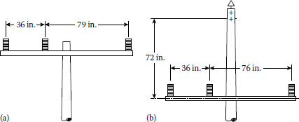
Various overhead pole-top conductor configurations: (a) without ground wire, z0 = z0,a and (b) with ground wire,
Example 10.2
Assume that a rural substation has a 3750 kVA 69/12.47 kV with LTC transformer feeding a three-phase four-wire 12.47 kV circuit protected by 140 A type L reclosers and 125 A series fuses. It is required to calculate the bolted fault current at point 10, 2 min from the substation on circuit 456319. Assume that the sizes of the phase conductors are 336AS37 (i.e., 336 kcmil bare-aluminum-steel conductors with 37 strands) and that neutral conductor is 0AS7, spaced 62 in. If the system impedance to the regulated 12.47 kV bus and the system impedance to ground are given as 0.7199 + j3.4619 Ω and 0.6191 + j3.3397 Ω, respectively, determine the following:
- The zero- and positive-sequence impedances of the line to point 10
- The impedance to ground of the line to point 10
- The total positive-sequence impedance to point 10 including system impedance to the regulated 12.47 kV bus.
- The total impedance to ground to point 10 including system impedance of the regulated 12.47 kV bus.
- The three-phase fault current at point 10
- The L-L fault current at point 10
- The line-to-ground fault current at point 10
Solution
- The zero-sequence impedance of the line to point 10 can be found by using Table 10.7 as
Similarly, the positive-sequence impedance of the line to point 10 can be found as
- From Equation 10.17, the impedance to ground of the line to point 10 is
- The total positive-sequence impedance is
- The total impedance to ground is
- From Equation 10.7, the three-phase fault at point 10 is
- From Equation 10.14, the L-L fault at point 10 is
- From Equation 10.15, the SLG fault at point 10 is
Sequence-Impedance Values Associated with Figure 10.26, Ω/1000 ft Conductor
Conductor |
||||
|---|---|---|---|---|
Size and Code |
Z1 = Z2 |
Z0,a |
Z'0 |
Z'' |
Bare-aluminum–steel (AS) | ||||
4AS7 |
0.4867 + j0.1613 |
0.5409 + j0.5195 |
0.0518 − j0.0543 |
0.0454 − j0.0493 |
4AS8 |
0.4830 + j0.1605 |
0.5372 + j0.5187 |
0.0520 − j0.0548 |
0.0456 − j0.0497 |
3AS7 |
0.3920 + j0.1617 |
0.4462 + j0.5198 |
0.0540 − j0.0685 |
0.0472 − j0.0620 |
2AS7 |
0.3202 + j0.1624 |
0.3743 + j0.5206 |
0.0535 − j0.0827 |
0.0465 − j0.0747 |
2AS8 |
0.3125 + j0.1581 |
0.3667 + j0.5162 |
0.0543 − j0.0846 |
0.0471 − j0.0764 |
1AS8 |
0.2614 + j0.1802 |
0.3156 + j0.5384 |
0.0459 − j0.0954 |
0.0395 − j0.0859 |
1AS7 |
0.2614 + j0.1624 |
0.3156 + j0.5206 |
0.0504 − j0.0970 |
0.0435 − j0.0874 |
0AS7 |
0.2121 + j0.1607 |
0.2663 + j0.5189 |
0.0451 − j0.1108 |
0.0385 − j0.0996 |
000AS7 |
0.1377 + j0.1541 |
0.1919 + j0.5123 |
0.0295 − j0.1346 |
0.0242 − j0.1206 |
267AS33 |
0.0729 + j0.1245 |
0.1271 + j0.4827 |
0.0092 − j0.1663 |
0.0056 − j0.1486 |
336AS37 |
0.0580 + j0.1208 |
0.1122 + j0.4789 |
0.0008 − j0.1722 |
-0.0020 − j0.1537 |
477AS33 |
0.0409 + j0.1168 |
0.0951+ j0.4789 |
-0.0101 − j0.1779 |
-0.0119 − j0.1587 |
636AS33 |
0.0306 + j0.1145 |
0.0848 + j0.4727 |
-0.0175 − j0.1807 |
-0.0184 − j0.1610 |
795AS33 |
0.0244 + j0.1120 |
0.0786 + j0.4702 |
-0.0221 − j0.1830 |
-0.0226 − j0.1630 |
Bare hard-drawn copper (X) | ||||
8X1 |
0.7194 + j0.1624 |
0.7739 + j0.5206 |
0.0432 − j0.0340 |
0.0380 − j0.0310 |
6X1 |
0.4527 + j0.1571 |
0.5069 + j0.5153 |
0.0535 − j0.0588 |
0.0468 − j0.0533 |
4X1 |
0.2875 + j0.1499 |
0.3417 + j0.5081 |
0.0554 − j0.0910 |
0.0480 − j0.0821 |
3X3 |
0.2280 + j0.1473 |
0.2822 + j0.5054 |
0.0513 − j0.1080 |
0.0441 − j0.0972 |
2X1 |
0.1790 + j0.1465 |
0.2332 + j0.5047 |
0.0432 − j0.1237 |
0.0366 − j0.1111 |
1X1 |
0.1420 + j0.1437 |
0.1962 + j0.5018 |
0.0342 − j0.1366 |
0.0283 − j0.1225 |
1X3 |
0.1432 + j0.1420 |
0.1976 + j0.5001 |
0.0352 − j0.1367 |
0.0292 − j0.1226 |
0X7 |
0.1150 + j0.1398 |
0.1692 + j0.4981 |
0.0255 − j0.1466 |
0.0205 − j0.1313 |
00X7 |
0.0911 + j0.1372 |
0.1453 + j0.4954 |
0.0156 − j0.1547 |
0.0115 − j0.1384 |
000X7 |
0.0723 + j0.1346 |
0.1265 + j0.4928 |
0.0065 − j0.1608 |
0.0033 − j0.1436 |
0000X7 |
0.0574 + j0.1317 |
0.1116 + j0.4899 |
0.0016 − j0.1654 |
-0.0041 − j0.1476 |
300X12 |
0.0407 + j0.1255 |
0.0949 + j0.4837 |
0.0114 − j0.1719 |
-0.0129 − j0.1532 |
Bare hard-drawn aluminum (AL) | ||||
0AL7 |
0.1843 + j0.1394 |
0.2385 + j0.4976 |
0.0468 − j0.1235 |
0.0398 − j0.1110 |
000AL7 |
0.1161 + j0.1345 |
0.1703 + j0.4927 |
0.0277 − j0.1485 |
0.0224 − j0.1330 |
267AL7 |
0.0731 + j0.1292 |
0.1273 + j0.4874 |
0.0082 − j0.1636 |
0.0047 − j0.1462 |
477AL19 |
0.0413 + j0.1212 |
0.0955 + j0.4794 |
-0.0105 − j0.1747 |
-0.0121 − j0.1558 |
Sequence-Impedance Values Associated with Figure 10.27, Ω/1000 ft
Conductor |
||||
|---|---|---|---|---|
Size and Code |
Z1 = Z2 |
Z0,a |
Z'0 |
Z'' |
Bare-aluminum-steel (AS) | ||||
4AS7 |
0.4867 + j0.1706 |
0.5229 + j0.3907 |
0.0338 − j0.0357 |
0.0279 − j0.0310 |
4AS8 |
0.4830 + j0.1698 |
0.5191 + j0.3900 |
0.0340 − j0.0360 |
0.0280 − j0.0313 |
3AS7 |
0.3920 + j0.1710 |
0.4282 + j0.3911 |
0.0353 − j0.0449 |
0.0289 − j0.0389 |
2AS7 |
0.3201 + j0.1717 |
0.3562 + j0.3919 |
0.0349 − j0.0542 |
0.0284 − j0.0468 |
2AS8 |
0.3125 + j0.1674 |
0.3486 + j0.3875 |
0.0354 − j0.0554 |
0.0288 − j0.0479 |
1 AS8 |
0.2614 + j0.1895 |
0.2975 + j0.4097 |
0.0299 − j0.0625 |
0.0240 − j0.0537 |
1AS7 |
0.2614 + j0.1717 |
0.2975 + j0.3919 |
0.0328 − j0.0636 |
0.0265 − j0.0547 |
0AS7 |
0.2121 + j0.1700 |
0.2483 + j0.3902 |
0.0293 − j0.0726 |
0.0233 − j0.0623 |
000AS7 |
0.1377 + j0.1634 |
0.1738 + j0.3836 |
0.0191 − j0.0882 |
0.0143 − j0.0753 |
267AS33 |
0.0729 + j0.1339 |
0.1090 + j0.3540 |
0.0057 − j0.1089 |
0.0024 − j0.0926 |
336AS33 |
0.0580 + j0.1301 |
0.0941 + j0.3502 |
0.0002 − j0.1127 |
-0.0023 − j0.0957 |
477AS33 |
0.0409 + j0.1261 |
0.0770 + j0.3462 |
-0.0070 − j0.1164 |
-0.0085 − j0.0987 |
636AS33 |
0.0306 + j0.1238 |
0.0668 + j0.3440 |
-0.0118 − j0.1182 |
-0.0126 − j0.1001 |
795AS33 |
0.0244 + j0.1214 |
0.0605 + j0.3415 |
-0.0148 − j0.1197 |
-0.0152 − j0.1013 |
Bare hard-drawn copper (X) | ||||
8X1 |
0.7197 + j0.1717 |
0.7558 + j0.3919 |
0.0282 − j0.0223 |
0.0234 − j0.0196 |
6X1 |
0.4527 + j0.1664 |
0.4888 + j0.3866 |
0.0349 − j0.0386 |
0.0288 − j0.0335 |
4X1 |
0.2847 + j0.1611 |
0.3208 + j0.3813 |
0.0357 − j0.0601 |
0.0289 − j0.0518 |
4X3 |
0.2875 + j0.1592 |
0.3236 + j0.3794 |
0.0361 − j0.0596 |
0.0293 − j0.0514 |
3X3 |
0.2280 + j0.1566 |
0.2642 + j0.3767 |
0.0334 − j0.0708 |
0.0268 − j0.0608 |
2X1 |
0.1790 + j0.1558 |
0.2151 + j0.3760 |
0.0281 − j0.0811 |
0.0220 − j0.0695 |
1X1 |
0.1420 + j0.1530 |
0.1782 + j0.3731 |
0.0221 − j0.0895 |
0.0168 − j0.0765 |
1X3 |
0.1434 + j0.1513 |
0.1795 + j0.3714 |
0.0228 − j0.0896 |
0.0173 − j0.0766 |
0X7 |
0.1150 + j0.1492 |
0.1511 + j0.3693 |
0.0164 − j0.0960 |
0.0118 − j0.0819 |
00X7 |
0.0911 + j0.1466 |
0.1272 + j0.3667 |
0.0099 − j0.1013 |
0.0062 − j0.0862 |
000X7 |
0.0723 + j0.1439 |
0.1085 + j0.3640 |
0.0040 − j0.1052 |
0.0010 − j0.0894 |
0000X7 |
0.0574 + j0.1411 |
0.0935 + j0.3612 |
-0.0014 − j0.1083 |
-0.0036 − j0.0919 |
300X12 |
0.0407 + j0.1348 |
0.0769 + j0.3550 |
-0.0078 − j0.1125 |
-0.0091 − j0.0953 |
Bare hard-drawn aluminum (AL) | ||||
0AL7 |
0.1843 + j0.1487 |
0.2204 + j0.3689 |
0.0304 − j0.0809 |
0.0240 − j0.0694 |
000AL7 |
0.1161 + j0.1438 |
0.1522 + j0.3640 |
0.0179 − j0.0972 |
0.0130 − j0.0830 |
267AL7 |
0.0731 + j0.1385 |
0.1092 + j0.3586 |
0.0050 − j0.1071 |
0.0019 − j0.0911 |
477AL19 |
0.0413 + j0.1306 |
0.0774 + j0.3507 |
-0.0072 − j0.1143 |
-0.0086 − j0.0969 |
Sequence-Impedance Values for Bare-Aluminum-Steel (AS) Associated with Figure 10.28, Ω/1000 ft
Conductor | |||
|---|---|---|---|
Size and Code |
Z1 = Z2 |
Z0,a |
Z'0 |
4AS8 |
0.4830 + j0.1605 |
0.5372 + j0.5187 |
0.0439 − j0.0484 |
0AS7 |
0.2121 + j0.1607 |
0.2663 + j0.5189 |
0.0368 − j0.0967 |
000AS7 |
0.1377 + j0.1541 |
0.1919 + j0.5123 |
0.0229 − j0.1169 |
267AS33 |
0.0729 + j0.1208 |
0.1122 + j0.4789 |
−0.0027 − j0.1489 |
477AS33 |
0.0409 + j0.1168 |
0.0951 + j0.4749 |
−0.0123 − j0.1536 |
636AS33 |
0.0306 + j0.1145 |
0.0848 + j0.4727 |
−0.0187 − j0.1558 |
795AS33 |
0.0244 + j0.1120 |
0.0786 + j0.4702 |
−0.0227 − j0.1577 |
Sequence-Impedance Values for Bare-Aluminum-Steel (AS) Associated with Figure 10.29, Ω/1000 ft
Conductor | |||
|---|---|---|---|
Size and Code |
Z1 = Z2 |
Z0,a |
Z'0 |
4AS8 |
0.4830 + j0.1660 |
0.5372 + j0.5077 |
0.0406 − j0.0458 |
0AS7 |
0.2121 + j0.1662 |
0.2663 + j0.5079 |
0.0334 − j0.0909 |
000AS7 |
0.1377 + j0.1596 |
0.1919 + j0.5012 |
0.0202 − j0.1097 |
267AS33 |
0.0729 + j0.1301 |
0.1271 + j0.4717 |
0.0029 − j0.1349 |
336AS37 |
0.0580 + j0.1263 |
0.1122 + j0.4679 |
-0.0040 − j0.1394 |
477AS33 |
0.0409 + j0.1223 |
0.0951 + j0.4639 |
-0.0131 − j0.1437 |
636AS33 |
0.0306 + j0.1200 |
0.0808 + j0.4617 |
-0.0191 − j0.1456 |
795AS33 |
0.0244 + j0.1176 |
0.0786 + j0.4592 |
-0.0229 − j0.1475 |
Impedance Values Associated with Figure 10.30, Ω/1000 ft
Conductor |
||
|---|---|---|
Size and Code |
|
|
Bare-aluminum–steel (AS) | ||
4AS7 |
0.5230 + j0.2618 |
0.5202 + j0.2640 |
4AS8 |
0.5193 + j0.2609 |
0.5165 + j0.2631 |
3AS7 |
0.4292 + j0.2572 |
0.4262 + j0.2601 |
2AS7 |
0.3570 + j0.2531 |
0.3540 + j0.2565 |
2AS8 |
0.3497 + j0.2481 |
0.3466 + j0.2516 |
1AS8 |
0.2957 + j0.2664 |
0.2929 + j0.2705 |
1AS7 |
0.2973 + j0.2481 |
0.2942 + j0.2522 |
0AS7 |
0.2462 + j0.2415 |
0.2433 + j0.2464 |
000AS7 |
0.1664 +j0.2265 |
0.1641 + j0.2326 |
267AS33 |
0.0946 +j0.1859 |
0.0930 + j0.1936 |
336AS37 |
0.0767 +j0.1800 |
0.0755 + j0.1880 |
477AS33 |
0.0559 +j0.1740 |
0.0551 + j0.1824 |
636AS33 |
0.0431 + j0.1708 |
0.0426 + j0.1793 |
795AS33 |
0.0352 + j0.1675 |
0.0349 + j0.1762 |
Bare hard-drawn copper (X) | ||
8X1 |
0.7529 + j0.2701 |
0.7507 + j0.2713 |
6X1 |
0.4895 + j0.2561 |
0.4866 + j0.2585 |
4X1 |
0.3221 + j0.2393 |
0.3189 + j0.2432 |
4X3 |
0.3251 + j0.2377 |
0.3219 + j0.2415 |
3X3 |
0.2643 + j0.2291 |
0.2611 + j0.2338 |
2X1 |
0.2124 + j0.2228 |
0.2096 + j0.2283 |
1X1 |
0.1724 + j0.2154 |
0.1698 + j0.2216 |
1X3 |
0.1740 + j0.2137 |
0.1715 + j0.2198 |
0X7 |
0.1423 + j0.2081 |
0.1401 + j0.2148 |
00X7 |
0.1150 + j0.2026 |
0.1132 + j0.2097 |
000X7 |
0.0931 + j0.1978 |
0.0916 + j0.2053 |
0000X7 |
0.0753 + j0.1934 |
0.0742 + j0.2011 |
300X 12 |
0.0552 + j0.1848 |
0.0546 + j0.1929 |
Bare hard-drawn aluminum (AL) | ||
0AL7 |
0.2190 + j0.2158 |
0.2159 + j0.2212 |
000AL7 |
0.1442 + j0.2021 |
0.1419 + j0.2089 |
267AL7 |
0.0944 + j0.1915 |
j0.1990 |
477AL 19 |
0.0557 + j0.1796 |
0.0554 + j0.1878 |
Note that the fault currents are calculated on the basis of a bolted fault. Therefore, they are accurate for faults caused by a low-impedance object making solid contact with the grounds.
However, usually the object causing the fault either has a high impedance or does not make solid contact with the conductors. This introduces an additional impedance into the circuit, which reduces the fault current to some value below the calculated value. Therefore, to be sure that the high-impedance faults will be cleared, it is crucial that all bolted faults clear within 3 s.