
Chapter 8
Application of Capacitors to Distribution Systems
Who neglects learning in his youth, loses the past and is dead for the future.
Euripides, 438 BC
Where is there dignity unless there is honesty?
Cicero
8.1 Basic Definitions
Capacitor element: an indivisible part of a capacitor consisting of electrodes separated by a dielectric material
Capacitor unit: an assembly of one or more capacitor elements in a single container with terminals brought out
Capacitor segment: a single-phase group of capacitor units with protection and control system Capacitor module: a three-phase group of capacitor segments
Capacitor bank: a total assembly of capacitor modules electrically connected to each other
8.2 Power Capacitors
At a casual look, a capacitor seems to be a very simple and unsophisticated apparatus, that is, two metal plates separated by a dielectric insulating material. It has no moving parts but instead functions by being acted upon by electric stress.
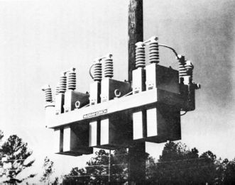
In reality, however, a power capacitor is a highly technical and complex device in that very thin dielectric materials and high electric stresses are involved, coupled with highly sophisticated processing techniques. Figure 8.1 shows a cutaway view of a power factor correction capacitor. Figure 8.2 shows a typical capacitor utilization in a switched pole-top rack.
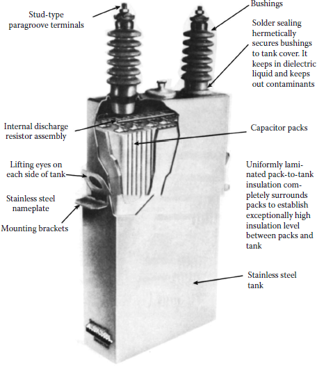
A cutaway view of a power factor correction capacitor.
(From McGraw-Edison Company, The ABC of Capacitors, Bulletin R230-90-1, 1968.)
In the past, most power capacitors were constructed with two sheets of pure aluminum foil separated by three or more layers of chemically impregnated kraft paper. Power capacitors have been improved tremendously over the last 30 years or so, partly due to improvements in the dielectric materials and their more efficient utilization and partly due to improvements in the processing techniques involved. Capacitor sizes have increased from the 15–25 kvar range to the 200–300 kvar range (capacitor banks are usually supplied in sizes ranging from 300 to 1800 kvar).
Nowadays, power capacitors are much more efficient than those of 30 years ago and are available to the electric utilities at a much lower cost per kilovar. In general, capacitors are getting more attention today than ever before, partly due to a new dimension added in the analysis: changeout economics. Under certain circumstances, even replacement of older capacitors can be justified on the basis of lower-loss evaluations of the modern capacitor design.
Capacitor technology has evolved to extremely low-loss designs employing the all-film concept; as a result, the utilities can make economic loss evaluations in choosing between the presently existing capacitor technologies.
8.3 Effects of Series and Shunt Capacitors
As mentioned earlier, the fundamental function of capacitors, whether they are series or shunt, installed as a single unit or as a bank, is to regulate the voltage and reactive power flows at the point where they are installed. The shunt capacitor does it by changing the power factor of the load, whereas the series capacitor does it by directly offsetting the inductive reactance of the circuit to which it is applied.
8.3.1 Series Capacitors
Series capacitors, that is, capacitors connected in series with lines, have been used to a very limited extent on distribution circuits due to being a more specialized type of apparatus with a limited range of application. Also, because of the special problems associated with each application, there is a requirement for a large amount of complex engineering investigation. Therefore, in general, utilities are reluctant to install series capacitors, especially of small sizes.
As shown in Figure 8.3, a series capacitor compensates for inductive reactance. In other words, a series capacitor is a negative (capacitive) reactance in series with the circuit’s positive (inductive) reactance with the effect of compensating for part or all of it. Therefore, the primary effect of the series capacitor is to minimize, or even suppress, the voltage drop caused by the inductive reactance in the circuit.

Voltage phasor diagrams for a feeder circuit of lagging power factor: (a) and (c) without and (b) and (d) with series capacitors.
At times, a series capacitor can even be considered as a voltage regulator that provides for a voltage boost that is proportional to the magnitude and power factor of the through current. Therefore, a series capacitor provides for a voltage rise that increases automatically and instantaneously as the load grows.
Also, a series capacitor produces more net voltage rise than a shunt capacitor at lower power factors, which creates more voltage drop. However, a series capacitor betters the system power factor much less than a shunt capacitor and has little effect on the source current.
Consider the feeder circuit and its voltage phasor diagram as shown in Figure 8.3a and c. The voltage drop through the feeder can be expressed approximately as
VD=IRcosθ+IXLsinθ(8.1)
where
R is the resistance of the feeder circuit
XL is the inductive reactance of the feeder circuit
cos θ is the receiving-end power factor
sin θ is the sine of the receiving-end power factor angle
As can be observed from the phasor diagram, the magnitude of the second term in Equation 8.1 is much larger than the first. The difference gets to be much larger when the power factor is smaller and the ratio of R/XL is small.
However, when a series capacitor is applied, as shown in Figure 8.3b and d, the resultant lower voltage drop can be calculated as
VD=IRcosθ+I(XL−XC)sinθ(8.2)
where Xc is the capacitive reactance of the series capacitor.
8.3.1.1 Overcompensation
Usually, the series-capacitor size is selected for a distribution feeder application in such a way that the resultant capacitive reactance is smaller than the inductive reactance of the feeder circuit. However, in certain applications (where the resistance of the feeder circuit is larger than its inductive reactance), the reverse might be preferred so that the resultant voltage drop is
VD=IRcosθ−I(XC−XL)sinθ(8.3)
The resultant condition is known as overcompensation. Figure 8.4a shows a voltage phasor diagram for overcompensation at normal load. At times, when the selected level of overcompensation is strictly based on normal load, the resultant overcompensation of the receiving-end voltage may not be pleasing at all because the lagging current of a large motor at start can produce an extraordinarily large voltage rise, as shown in Figure 8.4b, which is especially harmful to lights (shortening their lives) and causes light flicker, resulting in consumers’ complaints.

Overcompensation of the receiving-end voltage: (a) at normal load and (b) at the start of a large motor.
8.3.1.2 Leading Power Factor
To decrease the voltage drop considerably between the sending and receiving ends by the application of a series capacitor, the load current must have a lagging power factor. As an example, Figure 8.5a shows a voltage phasor diagram with a leading-load power factor without having series capacitors in the line. Figure 8.5b shows the resultant voltage phasor diagram with the same leading-load power factor but this time with series capacitors in the line. As can be seen from the figure, the receivingend voltage is reduced as a result of having series capacitors.

Voltage phasor diagram with leading power factor: (a) without series capacitors and (b) with series capacitors.
When cos θ = 1.0, sin θ ≅ 0, and therefore,
I(XL−XC)sinθ≅0
hence, Equation 8.2 becomes
VD≅IR(8.4)
Thus, in such applications, series capacitors practically have no value.
Because of the aforementioned reasons and others (e.g., ferroresonance in transformers, subsynchronous resonance during motor starting, shunting of motors during normal operation, and difficulty in protection of capacitors from system fault current), series capacitors do not have large applications in distribution systems.
However, they are employed in subtransmission systems to modify the load division between parallel lines. For example, often a new subtransmission line with larger thermal capability is parallel with an already existing line. It may be very difficult, if not impossible, to load the subtransmission line without overloading the old line. Here, series capacitors can be employed to offset some of the line reactance with greater thermal capability. They are also employed in subtransmission systems to decrease the voltage regulation.
8.3.2 Shunt Capacitors
Shunt capacitors, that is, capacitors connected in parallel with lines, are used extensively in distribution systems. Shunt capacitors supply the type of reactive power or current to counteract the outof-phase component of current required by an inductive load. In a sense, shunt capacitors modify the characteristic of an inductive load by drawing a leading current that counteracts some or all of the lagging component of the inductive load current at the point of installation. Therefore, a shunt capacitor has the same effect as an overexcited synchronous condenser, generator, or motor.
As shown in Figure 8.6, by the application of shunt capacitor to a feeder, the magnitude of the source current can be reduced, the power factor can be improved, and consequently the voltage drop between the sending end and the load is also reduced. However, shunt capacitors do not affect current or power factor beyond their point of application. Figure 8.6a and c shows the single-line diagram of a line and its voltage phasor diagram before the addition of the shunt capacitor, and Figure 8.6b and d shows them after the addition.

Voltage phasor diagrams for a feeder circuit of lagging power factor: (a) and (c) without and (b) and (d) with shunt capacitors.
Voltage drop in feeders, or in short transmission lines, with lagging power factor can be approximated as
VD=IRR+IXXL(8.5)
where
R is the total resistance of the feeder circuit, Ω
XL is the total inductive reactance of the feeder circuit, Ω
IR is the real power (or in-phase) component of the current, A
IX is the reactive (or out-of-phase) component of the current lagging the voltage by 90°, A
Example 8.1
Consider the right-angle triangle shown in Figure 8.7b. Determine the power factor of the load on a 460 V three-phase system, if the ammeter reads 100 A and the wattmeter reads 70 kW.
Solution
S=√3(V)(I)1000=√3(460 V)(100 A)1000≅79.67kVA
Thus,
PF=cos θ=PS=70 kW79.67 kVA≅0.88 or 88%
When a capacitor is installed at the receiving end of the line, as shown in Figure 8.6b, the resultant voltage drop can be calculated approximately as
VD=IRRR+IXXL−ICXL(8.6)
where Ic is the reactive (or out-of-phase) component of current leading the voltage by 90°, A.
The difference between the voltage drops calculated by using Equations 8.5 and 8.6 is the voltage rise due to the installation of the capacitor and can be expressed
VR=ICXL(8.7)
8.4 Power Factor Correction
8.4.1 General
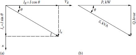
A typical utility system would have a reactive load at 80% power factor during the summer months. Therefore, in typical distribution loads, the current lags the voltage, as shown in Figure 8.7a. The cosine of the angle between current and sending voltage is known as the power factor of the circuit. If the in-phase and out-of-phase components of the current I are multiplied by the receiving-end voltage VR, the resultant relationship can be shown on a triangle known as the power triangle, as shown in Figure 8.7b. Figure 8.7b shows the triangular relationship that exists between kilowatts, kilovoltamperes, and kilovars.
Note that, by adding the capacitors, the reactive power component Q of the apparent power S of the load can be reduced or totally suppressed. Figures 8.8a and 8.9 illustrate how the reactive power component Q increases with each 10% change of power factor. Figure 8.8a also illustrates how a portion of lagging reactive power Qold is cancelled by the leading reactive power of capacitor Qc.

Illustration of (a) the use of a power triangle for power factor correction by employing capacitive reactive power and (b) the required increase in the apparent and reactive powers as a function of the load power factor, holding the real power of the load constant.

Illustration of the change in the real and reactive powers as a function of the load power factor, holding the apparent power of the load constant.
Note that, as illustrated in Figure 8.8, even an 80% power factor of the reactive power (kilovar) size is quite large, causing a 25% increase in the total apparent power (kilovoltamperes) of the line. At this power factor, 75 kvar of capacitors is needed to cancel out the 75 kvar of the lagging component.
As previously mentioned, the generation of reactive power at a power plant and its supply to a load located at a far distance is not economically feasible, but it can easily be provided by capacitors (or overexcited synchronous motors) located at the load centers. Figure 8.10 illustrates the power factor correction for a given system. As illustrated in the figure, capacitors draw leading reactive power from the source; that is, they supply lagging reactive power to the load. Assume that a load is supplied with a real power P, lagging reactive power Q1, and apparent power S1 at a lagging power factor of
cosθ1=PS1
or
cosθ1=P(P2+Q21)1/2(8.8)

When a shunt capacitor of Qc kVA is installed at the load, the power factor can be improved from cos θ1 to cos θ2, where
cosθ2=PS2=P(P2+Q22)1/2
or
cosθ2=P[P2+(Q1−QC)2]1/2(8.9)
8.4.2 Concept of Leading and Lagging Power Factors
Many consider that the terms “lagging” and “leading” power factor are somewhat confusing, and they are meaningless, if the directions of the flows of real and reactive powers are not known. In general, for a given load, the power factor is lagging if the load withdraws reactive power; on the other hand, it is leading if the load supplies reactive power.
Hence, an induction motor has a lagging power factor since it withdraws reactive power from the source to meet its magnetizing requirements. But a capacitor (or an overexcited synchronous motor) supplies reactive power and thus has a leading power factor, as shown in Figure 8.11 and indicated in Table 8.1.

Power Factor of Load and Source
Load Type |
At Load |
At Generator |
||||
|---|---|---|---|---|---|---|
P |
Q |
Power Factora |
P |
Q |
Power Factorb |
|
Induction motor |
In |
Out |
Lagging |
|||
Induction generator |
Out |
Out |
Lagging |
|||
Synchronous motor (Underexcited) |
In |
In |
Lagging |
Out |
Out |
Lagging |
Synchronous motor (Overexcited) |
In |
Out |
Leading |
Out |
In |
Leading |
a Power factor measured at the load.
b Power factor measured at the generator.
On the other hand, an underexcited synchronous motor withdraws both the real and reactive power from the source, as indicated. The use of varmeters instead of power factor meters avoids the confusion about the terms “lagging” and “leading.” Such a varmeter has a zero center point with scales on either side, one of them labeled “in” and the other one “out.”
8.4.3 Economic Power Factor
As can be observed from Figure 8.10b, the apparent power and the reactive power are decreased from S1 to S2 kVA and from Q1 to Q2 kvar (by providing a reactive power of Q), respectively. The reduction of reactive current results in a reduced total current, which in turn causes less power losses.
Thus, the power factor correction produces economic savings in capital expenditures and fuel expenses through a release of kilovoltamperage capacity and reduction of power losses in all the apparatus between the point of installation of the capacitors and the power plant source, including distribution lines, substation transformers, and transmission lines.
The economic power factor is the point at which the economic benefits of adding shunt capacitors just equal the cost of the capacitors. In the past, this economic power factor was around 95%. Today’s high plant and fuel costs have pushed the economic power factor toward unity.
However, as the corrected power factor moves nearer to unity, the effectiveness of capacitors in improving the power factor, decreasing the line kilovoltamperes transmitted, increasing the load capacity, or reducing line copper losses by decreasing the line current sharply decreases. Therefore, the correction of power factor to unity becomes more expensive with regard to the marginal cost of capacitors installed.
8.4.4 Use of a Power Factor Correction Table
Table 8.2 is a power factor correction table to simplify the calculations involved in determining the capacitor size necessary to improve the power factor of a given load from original to desired value. It gives a multiplier to determine the kvar requirement. It is based on the following formula:
Q=P(tanθorig−tanθnew)(8.10)
or
Q=P(√1PF2orig−1−√1PF2new−1)(8.11)
where
Q is the required compensation in kvar
P is the real power kW
PForig is the original power factor
PFnew is the desired power factor
Determination of kW Multiplies to Calculate kvar Requirement for Power Factor Correction
Reactive Factor |
Original Power Factor (%) |
Correcting Factor |
||||||||||||||||||||
|---|---|---|---|---|---|---|---|---|---|---|---|---|---|---|---|---|---|---|---|---|---|---|
Desired Power Factor (%) |
||||||||||||||||||||||
80 |
81 |
82 |
83 |
84 |
85 |
86 |
87 |
88 |
89 |
90 |
91 |
92 |
93 |
94 |
95 |
96 |
97 |
98 |
99 |
100 |
||
0.800 |
60 |
0.584 |
0.610 |
0.636 |
0.662 |
0.688 |
0.714 |
0.741 |
0.767 |
0.794 |
0.822 |
0.850 |
0.878 |
0.905 |
0.939 |
0.971 |
1.005 |
1.043 |
1.083 |
1.311 |
1.192 |
1.334 |
0.791 |
61 |
0.549 |
0.575 |
0.601 |
0.627 |
0.653 |
0.679 |
0.706 |
0.732 |
0.759 |
0.787 |
0.815 |
0.843 |
0.870 |
0.904 |
0.936 |
0.970 |
1.008 |
1.048 |
1.096 |
1.157 |
1.299 |
0.785 |
62 |
0.515 |
0.541 |
0.567 |
0.593 |
0.619 |
0.645 |
0.672 |
0.698 |
0.725 |
0.753 |
0.781 |
0.809 |
0.836 |
0.870 |
0.902 |
0.936 |
0.974 |
1.014 |
1.062 |
1.123 |
1.265 |
0.776 |
63 |
0.483 |
0.509 |
0.535 |
0.561 |
0.587 |
0.613 |
0.640 |
0.666 |
0.693 |
0.721 |
0.749 |
0.777 |
0.804 |
0.838 |
0.870 |
0.904 |
0.942 |
0.982 |
1.030 |
1.091 |
1.233 |
0.768 |
64 |
0.450 |
0.476 |
0.502 |
0.528 |
0.554 |
0.580 |
0.607 |
0.633 |
0.660 |
0.688 |
0.716 |
0.744 |
0.771 |
0.805 |
0.837 |
0.871 |
0.909 |
0.949 |
0.997 |
1.058 |
1.200 |
0.759 |
65 |
0.419 |
0.445 |
0.471 |
0.479 |
0.523 |
0.549 |
0.576 |
0.602 |
0.629 |
0.657 |
0.685 |
0.713 |
0.740 |
0.774 |
0.806 |
0.840 |
0.878 |
0.918 |
0.966 |
1.027 |
1.169 |
0.751 |
66 |
0.388 |
0.414 |
0.440 |
0.466 |
0.492 |
0.518 |
0.545 |
0.571 |
0.598 |
0.626 |
0.654 |
0.682 |
0.709 |
0.743 |
0.775 |
0.809 |
0.847 |
0.887 |
0.935 |
0.996 |
1.138 |
0.744 |
67 |
0.358 |
0.384 |
0.410 |
0.436 |
0.462 |
0.488 |
0.515 |
0.541 |
0.568 |
0.596 |
0.624 |
0.652 |
0.679 |
0.713 |
0.745 |
0.779 |
0.817 |
0.857 |
0.905 |
0.966 |
1.108 |
0.733 |
68 |
0.329 |
0.355 |
0.381 |
0.407 |
0.433 |
0.459 |
0.486 |
0.512 |
0.539 |
0.567 |
0.595 |
0.623 |
0.650 |
0.684 |
0.716 |
0.750 |
0.788 |
0.828 |
0.876 |
0.937 |
1.079 |
0.725 |
69 |
0.299 |
0.325 |
0.351 |
0.377 |
0.403 |
0.429 |
0.456 |
0.482 |
0.509 |
0.537 |
0.565 |
0.593 |
0.620 |
0.654 |
0.686 |
0.720 |
0.758 |
0.798 |
0.840 |
0.907 |
1.049 |
0.714 |
70 |
0.270 |
0.296 |
0.322 |
0.348 |
0.374 |
0.400 |
0.427 |
0.453 |
0.480 |
0.508 |
0.536 |
0.564 |
0.591 |
0.625 |
0.657 |
0.691 |
0.729 |
0.769 |
0.811 |
0.878 |
1.020 |
0.704 |
71 |
0.242 |
0.268 |
0.294 |
0.320 |
0.346 |
0.372 |
0.399 |
0.425 |
0.452 |
0.480 |
0.508 |
0.536 |
0.563 |
0.597 |
0.629 |
0.663 |
0.700 |
0.741 |
0.783 |
0.850 |
0.992 |
0.694 |
72 |
0.213 |
0.239 |
0.265 |
0.291 |
0.317 |
0.343 |
0.370 |
0.396 |
0.423 |
0.451 |
0.479 |
0.507 |
0.534 |
0.568 |
0.600 |
0.634 |
0.672 |
0.712 |
0.754 |
0.821 |
0.963 |
0.682 |
73 |
0.186 |
0.212 |
0.238 |
0.264 |
0.290 |
0.316 |
0.343 |
0.369 |
0.396 |
0.424 |
0.452 |
0.480 |
0.507 |
0.541 |
0.573 |
0.607 |
0.645 |
0.685 |
0.727 |
0.794 |
0.936 |
0.673 |
74 |
0.159 |
0.185 |
0.211 |
0.237 |
0.263 |
0.289 |
0.316 |
0.342 |
0.369 |
0.397 |
0.425 |
0.453 |
0.480 |
0.514 |
0.546 |
0.580 |
0.618 |
0.658 |
0.700 |
0.767 |
0.909 |
0.661 |
75 |
0.132 |
0.158 |
0.184 |
0.210 |
0.236 |
0.262 |
0.289 |
0.315 |
0.342 |
0.370 |
0.398 |
0.426 |
0.453 |
0.487 |
0.519 |
0.553 |
0.591 |
0.631 |
0.673 |
0.740 |
0.882 |
0.650 |
76 |
0.105 |
0.131 |
0.157 |
0.183 |
0.209 |
0.235 |
0.262 |
0.288 |
0.315 |
0.343 |
0.371 |
0.399 |
0.426 |
0.460 |
0.492 |
0.526 |
0.564 |
0.604 |
0.652 |
0.713 |
0.855 |
0.637 |
77 |
0.079 |
0.105 |
0.131 |
0.157 |
0.183 |
0.209 |
0.236 |
0.262 |
0.289 |
0.317 |
0.345 |
0.373 |
0.400 |
0.434 |
0.466 |
0.500 |
0.538 |
0.578 |
0.620 |
0.687 |
0.829 |
0.626 |
78 |
0.053 |
0.079 |
0.105 |
0.131 |
0.157 |
0.183 |
0.210 |
0.236 |
0.263 |
0.291 |
0.319 |
0.347 |
0.374 |
0.408 |
0.440 |
0.474 |
0.512 |
0.552 |
0.594 |
0.661 |
0.803 |
0.613 |
79 |
0.026 |
0.052 |
0.078 |
0.104 |
0.130 |
0.156 |
0.183 |
0.209 |
0.236 |
0.264 |
0.292 |
0.320 |
0.347 |
0.381 |
0.413 |
0.447 |
0.485 |
0.525 |
0.567 |
0.634 |
0.776 |
0.600 |
80 |
0.000 |
0.026 |
0.052 |
0.078 |
0.104 |
0.130 |
0.157 |
0.183 |
0.210 |
0.238 |
0.266 |
0.294 |
0.321 |
0.355 |
0.387 |
0.421 |
0.459 |
0.499 |
0.541 |
0.608 |
0.750 |
0.588 |
81 |
0.000 |
0.026 |
0.052 |
0.078 |
0.104 |
0.131 |
0.157 |
0.184 |
0.212 |
0.240 |
0.268 |
0.295 |
0.329 |
0.361 |
0.395 |
0.433 |
0.473 |
0.515 |
0.528 |
0.724 |
|
0.572 |
82 |
0.000 |
0.026 |
0.052 |
0.078 |
0.105 |
0.131 |
0.158 |
0.186 |
0.214 |
0.242 |
0.269 |
0.303 |
0.335 |
0.369 |
0.407 |
0.447 |
0.489 |
0.556 |
0.698 |
||
0.559 |
83 |
0.000 |
0.026 |
0.052 |
0.079 |
0.105 |
0.132 |
0.160 |
0.188 |
0.216 |
0.243 |
0.277 |
0.309 |
0.343 |
0.381 |
0.421 |
0.463 |
0.530 |
0.672 |
|||
0.543 |
84 |
0.000 |
0.026 |
0.053 |
0.079 |
0.106 |
0.134 |
0.162 |
0.190 |
0.217 |
0.251 |
0.283 |
0.317 |
0.355 |
0.395 |
0.437 |
0.504 |
0.646 |
||||
0.529 |
85 |
0.000 |
0.027 |
0.053 |
0.080 |
0.108 |
0.136 |
0.164 |
0.191 |
0.225 |
0.257 |
0.291 |
0.329 |
0.369 |
0.417 |
0.478 |
0.620 |
|||||
0.510 |
86 |
0.000 |
0.026 |
0.053 |
0.081 |
0.109 |
0.137 |
0.167 |
0.198 |
0.230 |
0.265 |
0.301 |
0.342 |
0.390 |
0.451 |
0.593 |
||||||
0.497 |
87 |
0.000 |
0.027 |
0.055 |
0.083 |
0.111 |
0.141 |
0.172 |
0.204 |
0.239 |
0.275 |
0.316 |
0.364 |
0.425 |
0.567 |
|||||||
0.475 |
88 |
0.000 |
0.028 |
0.056 |
0.083 |
0.113 |
0.144 |
0.176 |
0.211 |
0.247 |
0.288 |
0.336 |
0.397 |
0.540 |
||||||||
0.455 |
89 |
0.000 |
0.028 |
0.055 |
0.086 |
0.117 |
0.149 |
0.183 |
0.221 |
0.262 |
0.309 |
0.370 |
0.512 |
|||||||||
0.443 |
90 |
0.000 |
0.028 |
0.058 |
0.089 |
0.121 |
0.155 |
0.193 |
0.234 |
0.281 |
0.342 |
0.484 |
||||||||||
0.427 |
91 |
0.000 |
0.030 |
0.061 |
0.093 |
0.127 |
0.165 |
0.206 |
0.253 |
0.314 |
0.456 |
|||||||||||
0.392 |
92 |
0.000 |
0.031 |
0.063 |
0.097 |
0.135 |
0.176 |
0.223 |
0.284 |
0.426 |
||||||||||||
0.386 |
93 |
0.000 |
0.032 |
0.066 |
0.104 |
0.145 |
0.192 |
0.253 |
0.395 |
|||||||||||||
0.341 |
94 |
0.000 |
0.035 |
0.072 |
0.113 |
0.160 |
0.221 |
0.363 |
||||||||||||||
0.327 |
95 |
0.000 |
0.036 |
0.078 |
0.125 |
0.186 |
0.328 |
|||||||||||||||
0.280 |
96 |
0.000 |
0.041 |
0.089 |
0.150 |
0.292 |
||||||||||||||||
0.242 |
97 |
0.000 |
0.048 |
0.109 |
0.251 |
|||||||||||||||||
0.199 |
98 |
0.000 |
0.061 |
0.203 |
||||||||||||||||||
0.137 |
99 |
0.000 |
0.142 |
|||||||||||||||||||
8.4.5 Alternating Cycles of a Magnetic Field
Furthermore, in order to understand how the power factor of a device can be improved, one has to understand what is taking place electrically. Consider an induction motor that is being supplied by the real power P and the reactive power Q. The real power P is lost, whereas the reactive power Q is not lost. But instead it is used to store energy in the magnetic field of the motor.
Since the current is alternating, the magnetic field undergoes cycles of building up and breaking down. As the field is building up, the reactive current flows from the supply or source to the motor. As the field is breaking down, the reactive current flows out of the motor back to the supply or source. In such application, what is needed is some type of device that can be used as a temporary storage area for the reactive power when the magnetic field of the motor breaks down.
The ideal device for this is a capacitor that also stores energy. However, this energy is stored in an electric field. By connecting a capacitor in parallel with the supply line of the load, the cyclic flow of reactive power takes place between the motor and the capacitor. Here, the supply lines carry only the current supplying real power to the motor. This is only applicable for a unity power factor condition. For other power factors, the supply lines would carry some reactive power.
8.4.6 Power Factor of a Group of Loads
In general, the power factor of a single load is known. However, it is often that the power factor of a group of various loads needs to be determined. This is accomplished based on the known power relationship.
Example 8.2
Assume that a substation supplies three different kinds of loads, mainly, incandescent lights, induction motors, and synchronous motors, as shown in Figure 8.12. The substation power factor is found from the total reactive and real powers of the various loads that are connected. Based on the given data in Figure 8.12, determine the following:
- The apparent, real, and kvars of each load
- The total apparent, real, and reactive powers of the power that should be supplied by the substation
- The total power factor of the substation
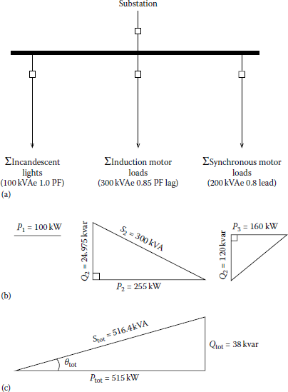
For Example 8.2: (a) connection diagram, (b) phasor diagrams of individual loads, and (c) phasor diagram of combined loads.
Solution
-
- For a 100 kVA lighting load
Since incandescent lights are basically a unity power factor load, it is assumed that all the current is kilowatt current. Hence,
S1=P1100 kVA≅100 kW
- For 400 hp of connected induction motor loads
Assume that for the motor loads,
kVA load = 0.75×(Connected motor horse power)
with an opening power factor of 85% lagging:
S2=(0.75kWhp)(400 hp)=300 kVA
P3=(0.75 × 400) × 0.85=255 kW
Q2=√(300)2−(255)2=√90,000−65,025=24,975≅158 kvar
- 200 hp motor with a 0.8 leading power factor
At full load, assume kVA = motor-hp rating = 200 kVA:
P3=(200 kVA)cosθ=200×0.8=160kW
Q2=√(200 kVA)2−(160 kW)2=√40,000−25,600=√14,400=120 kavr
- For a 100 kVA lighting load
- At the substation, the total real power is
Ptotal=Plights+Pind.mot.+Psync.mot.=100+255+160=515 kW
The total reactive power is
Qtotal=Qlights+Qind.mot.=0+158=158 kvar
Thus, an overexcited synchronous motor operating without the mechanical load connected to its shaft can supply the leading reactive power. Hence, the net lagging reactive power that must be supplied by the substation is the difference between the reactive power supplied by the synchronous motor and the reactive power required by the induction motor loads:
Induction motor load required = 158
kvar Synchronous motor supplied = 120
kvar Substation must supply = 38 kvar
- The kVA of the substation is
Stotal=√P2tot+Q2tot(8.12)
or
Stotal=√5152+382=√266,669=516.4 kVA
The power factor of the substation is
PF = power factor=PS=515 kW516.4 kVA=0.997 lagging
8.4.7 Practical Methods Used by the Power Industry for Power Factor Improvement Calculations
It is often that the formulas that are used by the power industry contains kW, kVA, or kvar instead of the symbols of P, S, Q, which are the correct form and used in the academia. However, there are certain advantages of using them since one does not have to think which one is P, S, or Q.
From the right-triangle relationship, several simple and useful mathematical expressions may be written as
PF=cosθ=kWkVA(8.13)
tanθ=kvarkW(8.14)
sinθ=kvarkVA(8.15)
Since the kW component normally stays the same (the kVA and kvar components change with power factor), it is convenient to use Equation 8.11 involving the kW component. The relationship can be reexpressed as
kvar = kW×tanθ(8.16)
For instance, if it is necessary to determine the capacitor rating to improve the load’s power factor, one would use the following relationships:
kvar at original PF = kW × tanθ1(8.17)
kvar at improved PF = kW × tanθ2(8.18)
Thus, the capacitor rating required to improve the power factor can be expressed as
ckvar* = kW × (tanθ1−tanθ2)(8.19)
or
Δtanθ=tanθ1−tanθ2(8.20)
then
ckvar* = kW×Δtanθ(8.21)
Table 8.2 has a “kW multiplier” for determining the capacitor based on the previously mentioned expression. Also, note that the prefix “c” in ckvar is employed to designate the capacitor kvar in order to differentiate it from load kvar.
To find irrespective currents of kVA, kW, and kvar, use the following relationships:
kVA = √(kW)2+(kvar)2(8.22)
kW = √(kVA)2+(kvar)2(8.23)
kvar = √(kVA)2+(kW)2(8.24)
Example 8.3
Assume that a load withdraws 80 kW and 60 kvar at a 0.8 power factor. It is required that its power factor is to be improved from 80% to 90% by using capacitors. Determine the amount of the reactive power to be provided by using capacitors.
Solution
Without capacitors at PF = 0.8
kW=80kvar=60
Thus, the kVA requirement of the load is
kVA = (802 + 602)1/2 = 100 kVA
With capacitors at PF = 0.9
kW=80kVA≅88.9
Line kvar = (88.92 – 802)1/2 (7903–s6400)1/2 = 38.7
Hence, the line supplies 38.7 kvar and the load needs 60 kvar, and the capacitor supplies the difference, or
ckvar = 60−38.7=21.3 kvar
as it is illustrated in Figure 8.13.

Example 8.4
Determine the capacitor rating in Example 8.3 by using Table 8.2.
Solution
From Table 8.2, the "kW multiplier" or Δ tan θ is read as 0.266. Therefore,
ckvar=kW×Δtanθ=(80 kW)×(0.266)=21.3 kvar
which is the same value determined by the calculation in Example 8.3.
Example 8.5
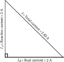
Assume that a certain load withdraws a kilowatt current of 2 A and kilovar current of 2 A. Determine the amount of total current that it withdraws.
Solution
The answer is not the following!
(2 A) + (2 A) = 4 A
The correct answer can be found from the following right-triangle relationships:
(kvar current)2 + (kW current)2 = (total current)2
(2 A)2 + (2 A)2 = (total current)2
or
4 + 4 = (total current)2
Hence,
Total current = 81/2 = 2.83 A
Thus,
2 + 2 ≠ 4!
Figure 8.14 shows the component current diagram.
Example 8.6
Assume that a 460 V cable circuit is rated at 240 A but is carrying a load of 320 A at 0.65 power factor. Determine the kvar of capacitor that is needed to reduce the current to 240 A.
Solution
kVA=√3 × (460 V) × (320 A)=254.96 kVAkW=(254.96 kVA)0.65=165.72 kW
The kVA corresponding to 240 A is
kVA=√3×(460 V)(240 A)1000=191.2 kVA
Thus, the operating power factor corresponding to the new load is
PF2=cosθ2=PS2=165.72 kW191.2 kVA=0.8667
The capacitor kvar required is
ckvar=(165.72 kW) tan(cos−1 0.8667)=(165.72 kW) tan(29.92°)≅(165.72)(0.5755)≅95.38
8.4.8 Real Power-Limited Equipment
Certain equipments such as turbogenerator (i.e., turbine generators) and engine generator sets have a real power (P) limit of the prime mover as well as a kVA limit of the generator. Usually the real power limit corresponds to the generator S rating, and the set is rated at that P value at unity power factor operation.
Other real power (P) values that correspond to the lesser power factor operations are determined by the power factor and real power (S) rating at the generator in order that the P and S ratings of the load do not exceed the S rating of the generator. Any improvement of the power factor can release both P and S capacities.
Example 8.7
Assume that a 1000 kW turbine unit (turbogenerator set) has a turbine capability of 1250 kW. It is operating at a rated load of 1250 kVA at 0.85 power factor. An additional load of 150 kW at 0.85 power factor is to be added. Determine the value of capacitors needed in order not to overload the turbine nor the generator.
Solution
Original load
P=1000 kWQ=√(kVA)2−(kW)2=√(1250)2−(1000)2=750 kvar
Additional load
P=kW=150 kW
S=kVA=150 kW0.85=200 kVA
Q=√(200)2−(1000)2=132.29 kvar
Total load
Ptot=kW=1000+150=1150 kW
Qtot=750+132.29=882.29 kvar
The minimum operating power factor for a load of 1150 kW and not exceeding the kVA rating of the generator is
PF=cosθ=1150 kW1250 kVA=0.92
The maximum load kvar for this situation is
Q=(1150 kW)tan−1θ=1150×tan−1(23.073918°)≅489.9 kvar
where 0.426 is the tangent corresponding to the maximum power factor of 0.935.
Thus, the capacitors must provide the difference between the total load kvar and the permissible generator kvar, or
ckvar=882.29−489.9=392.39 kvar
Example 8.8
Assume that a 700 k VA load has a 65% power factor. It is desired to improve the power factor to 92%. Using Table 8.2, determine the following:
- The correction factor required.
- The capacitor size required.
- What would be the resulting power factor if the next higher standard capacitor size is used? Solution
Solution
- From Table 8.2, the correction factor required can be found as 0.74.
- The 700 kVA load at 65% power factor is
PL=SL×cosθ=700×0.65=455 kW(8.25)
The capacitor size necessary to improve the power factor from 65% to 92% can be found as
Capacitor size=PL(correlation factor)=455(0.74)=336.7 kvar(8.26)
- Assume that the next higher standard capacitor size (or rating) is selected to be 360 kvar. Therefore, the resulting new correction factor can be found from
New correction factor=Standard capacitor ratingPL=360 kvar455 kW=0.7912(8.27)
From the table by linear interpolation, the resulting corrected percent power factor, with an original power factor of 65% and a correction factor of 0.7912, can be found as
New corrected%power factor=93+172320≅93.5
8.4.9 Computerized Method to Determine the Economic Power Factor
As suggested by Hopkinson [1], a load flow digital computer program can be employed to determine the kilovoltamperes, kilovolts, and kilovars at annual peak level for the whole system (from generation through the distribution substation buses) as the power factor is varied.
As a start, shunt capacitors are applied to each substation bus for correcting to an initial power factor, for example, 90%. Then, a load flow run is performed to determine the total system kilovoltamperes, and kilowatt losses (from generator to load) at this level and capacitor kilovars are noted. Later, additional capacitors are applied to each substation bus to increase the power factor by 1%, and another load flow run is made. This process of iteration is repeated until the power factor becomes unity.
As a final step, the benefits and costs are calculated at each power factor. The economic power factor is determined as the value at which benefits and costs are equal. After determining the economic power factor, the additional capacitor size required can be calculated as
ΔQc=PPK(tanϕ−tanθ)(8.28)
where
ΔQc is the required capacitor size, kvar
PPK is the system demand at annual peak, kW
tan ɸ is the tangent of original power factor angle
tan θ is the tangent of economic power factor angle
An illustration of this method is given in Example 8.12.
8.5 Application of Capacitors
In general, capacitors can be applied at almost any voltage level. As illustrated in Figure 8.15, individual capacitor units can be added in parallel to achieve the desired kilovar capacity and can be added in series to achieve the required kilovolt voltage. They are employed at or near rated voltage for economic reasons.

The cumulative data gathered for the whole utility industry indicate that approximately 60% of the capacitors is applied to the feeders, 30% to the substation buses, and the remaining 10% to the transmission system [1].
The application of capacitors to the secondary systems is very rare due to small economic advantages. Zimmerman [3] has developed a nomograph, shown in Figure 8.16, to determine the economic justification, if any, of the secondary capacitors considering only the savings in distribution transformer cost.

Secondary capacitor economics considering only savings in distribution transformer cost.
(From Zimmerman, R.A., AIEE Trans., 72, 694, Copyright 1953 IEEE. Used with permission.)
Example 8.9
Assume that a three-phase 500 hp 60 Hz 4160 V wye-connected induction motor has a fullload efficiency (η) of 88% and a lagging power factor of 0.75 and is connected to a feeder. If it is desired to correct the power factor of the load to a lagging power factor of 0.9 by connecting three capacitors at the load, determine the following:
- The rating of the capacitor bank, in kilovars
- The capacitance of each unit if the capacitors are connected in delta, in microfarads
- The capacitance of each unit if the capacitors are connected in wye, in microfarads
Solution
- The input power of the induction motor can be found as
P=(HP)(0.7457 kW/hp)η=(500 hp)(0.7457 kW/hp)0.88=423.69 kW
The reactive power of the motor at the uncorrected power factor is
Q1=Ptanθ1=423.69tan (cos−1 0.75)=423.69×0.8819=373.7 kvar
The reactive power of the motor at the corrected power factor is
Q2=Ptanθ2=423.69tan (cos−1 0.90)=423.69×0.4843=205.2 kvar
Therefore, the reactive power provided by the capacitor bank is
QC=Q1−Q2=373.7−205.2=168.5 kvar
Hence, assuming the losses in the capacitors are negligible, the rating of the capacitor bank is 168.5 kvar.
- If the capacitors are connected in delta as shown in Figure 8.17a, the line current is
IL=QC√3×VL−L=168.5√3×4.16=23.39 A
and therefore,
IC=IL√3=23.39√3=13.5 A
Thus, the reactance of each capacitor is
XC=VL−LIC=416013.5=308.11 Ω
and hence, the capacitance of each unit,* if the capacitors are connected in delta, is
C=106ωXCμF
or
C=106ωXC=1062π×60×308.11=8.61μF
- If the capacitors are connected in wye as shown in Figure 8.17b,
IC=IL=23.39A
and therefore,
XC=VL−NIC=4160√3×23.39=102.70 Ω
Thus, the capacitance of each unit, if the capacitors are connected in wye, is
C=106ωXC=1062π×60×102.70=25.82 μF
C=1/(ωXC)F.
C=106/(ωXC)(10−6F)
C=106/(ωXC) μF: C/106=(1/ωXC)/106F

Example 8.10
Assume that a 2.4 kV single-phase circuit feeds a load of 360 kW (measured by a wattmeter) at a lagging load factor and the load current is 200 A. If it is desired to improve the power factor, determine the following:
- The uncorrected power factor and reactive load.
- The new corrected power factor after installing a shunt capacitor unit with a rating of 300 kvar.
- Also write the necessary codes to solve the problem in MATLAB®.
Solution
- Before the power factor correction,
S1=V×I=2.4×200=480 kVA
therefore, the uncorrected power factor can be found as
cosθ1=PS1=360 kW480 kVA=0.75
and the reactive load is
Q1=S1×sin(cos−1 θ1)=480×0.661=317.5 kvar
- After the installation of the 300 kvar capacitors,
Q2=Q1−QC=317.5−300=17.5 kvar
and therefore, the new power factor can be found from Equation 8.9 as
cosθ2=P[P2+(Q1−QC)2]1/2=360(3602+17.52)1/2=0.9989 or 99.89%
- Here is the MATLAB script:
clcclear% System parametersHP = 500;PFold = 0.75;PFnew = 0.90;effi = 0.88;kVL = 4.16;VL = 4160;% Solution for part a% Solve for input power of motor in kWP = (HP*0.7457)/effi% Solve for reactive power of motor in kvarQ1 = P*tan(acos(PFold))% Reactive power of motor at corrected power factor in kvarQ2 = P*tan(acos(PFnew))% Reactive power provided by capacitor bank in kvarQc = Q1 - Q2% Solution for part b when capacitors are in delta% Line current when capacitors are in delta, in AmpsIL = Qc/(sqrt(3)*kVL)% Capacitor current in AmpsIc = IL/sqrt(3)% Reactance of each capacitor in ohmsXc = VL/Ic% Capacitance of each unit in micro faradsC = (10^6)/(120*pi*Xc)% Solution for part c when capacitors are in wye% Capacitance current is equal to line current when capacitors are in wye% Reactance of each capacitor in ohmsXcwye = VL/(sqrt(3)*IL)% Capacitance of each unit in micro faradsCwye = (10^6)/(120*pi*Xcwye)
Example 8.11
Assume that the Riverside Substation of the NL&NP Company has a bank of three 2000 kVA transformers that supplies a peak load of 7800 kVA at a lagging power factor of 0.89. All three transformers have a thermal capability of 120% of the nameplate rating. It has already been planned to install 1000 kvar of shunt capacitors on the feeder to improve the voltage regulation.
Determine the following:
- Whether or not to install additional capacitors on the feeder to decrease the load to the thermal capability of the transformer
- The rating of the additional capacitors
Solution
- Before the installation of the 1000 kvar capacitors,
P=S1×cosθ=7800×0.89=6942 kW
and
Q1=S1×sinθ=7800×0.456=3556.8 kvar
Therefore, after the installation of the 1000 kvar capacitors,
Q2=Q1−QC=3556.8−1000=2556.8 kvar
and using Equation 8.9,
cosθ2=P[P2+(Q1−QC)2]1/2=6942(69422+2556.82)1/2=0.938 or 93.8%
and the corrected apparent power is
S2=Pcosθ2=69420.938=7397.9 kVA
On the other hand, the transformer capability is
ST=6000×1.20=72000 kVA
Therefore, the capacitors installed to improve the voltage regulation are not adequate; additional capacitor installation is required.
- The new or corrected power factor required can be found as
PF2,new=cosθ2,new=PST=69427200=0.9642 or 96.42%
and thus, the new required reactive power can be found as
Q2,new=P×tanθ2,new=P×tan(cos−1PF2,new)=6942×0.2752=1910 kvar
Therefore, the rating of the additional capacitors required is
QC,add=Q2−Q2,new=2556.8−1910=646.7 kvar
Example 8.12
If a power system has 10,000 kVA capacity and is operating at a power factor of 0.7 and the cost of a synchronous capacitor (i.e., synchronous condenser) to correct the power factor is $10 per kVA, find the investment required to correct the power factor to
- 0.85 lagging power factor
- Unity power factor
Solution
At original cost
θold=cos−1PF = cos−1 0.7=45.57°
Pold=Scosθold=(10,000 kVA)0.7 =7,000 kW
Qold=Ssinθold=(10,000 kVA)sin45.57°=7,141.43 kvar
- For PF = 0.85 lagging
Pnew=Pold=7000 kW (as before)Snew=Pnewcosθnew=7000kW0.85=8235.29 kVA
Qnew=Snewsin(cos−1PF)=(8235.29 kVA)sin(cos−10.85)=4338.21 kvar
Hence, the theoretical cost of the synchronous capacitor is
Note that it is customary to give the cost of capacitors in dollars per kVA rather than in dollars per kvar.
- For PF = 1.0
Thus, the theoretical cost of the synchronous capacitor is
Note that Pnew = 7000 kW is the same as before.
Example 8.13
If a power system has 15,000 kVA capacity, operating at a 0.65 lagging power factor, and the cost of synchronous capacitors to correct the power factor is $12.5/kVA, determine the costs involved and also develop a table showing the required (leading) reactive power to increase the power factor to
- 0.85 lagging power factor
- 0.95 lagging power factor
- Unity power factor
Solution
At original power factor or 0.65
The following table shows the amount of reactive power that is required to improve the power factor from one level to the next at 0.05 increments.
PF |
P (kW) |
Q (kvar) |
Q to Correct from Next Lower PF (kvar) |
Cumulative Q Required for Correction (kvar) |
|---|---|---|---|---|
0.65 |
9,750 |
11,399 |
— |
— |
0.70 |
10,500 |
10,712 |
687 |
687 |
0.75 |
11,250 |
9,922 |
790 |
1,477 |
0.80 |
12,000 |
9,000 |
922 |
2,399 |
0.85 |
12,750 |
7,902 |
1098 |
3,497 |
0.90 |
13,500 |
6,538 |
1364 |
4,861 |
0.95 |
14,250 |
4,684 |
1854 |
6,715 |
1.00 |
15,000 |
0 |
4684 |
11,399 |
- For PF = 0.85 lagging
P = S cos θ = (15,000 kVA) × 0.65 = 9,750 kW. It will be the same at a power factor of 0.85.
and
amount of additional reactive power correction required is
The cost of this correction is
- For PF = 0.95 lagging:
and
The amount of additional reactive power correction required is
The cost of this correction is
- For unity PF
The amount of additional reactive power correction required is
The cost of this correction is
8.5.1 Capacitor Installation Types
In general, capacitors installed on feeders are pole-top banks with necessary group fusing. The fusing applications restrict the size of the bank that can be used. Therefore, the maximum sizes used are about 1800 kvar at 15 kV and 3600 kvar at higher voltage levels. Usually, utilities do not install more than four capacitor banks (of equal sizes) on each feeder.
Figure 8.18 illustrates the effects of a fixed capacitor on the voltage profiles of a feeder with uniformly distributed load at heavy load and light load. If only fixed-type capacitors are installed, as can be observed in Figure 8.18c, the utility will experience an excessive leading power factor and voltage rise at that feeder. Therefore, as shown in Figure 8.19, some of the capacitors are installed as switched capacitor banks so they can be switched off during light-load conditions.

The effects of a fixed capacitor on the voltage profile of (a) feeder with uniformly distributed load (b) at heavy load and (c) at light load.
Thus, the fixed capacitors are sized for light load and connected permanently. As shown in the figure, the switched capacitors can be switched as a block or in several consecutive steps as the reactive load becomes greater from light-load level to peak load and sized accordingly.
However, in practice, the number of steps or blocks is selected to be much less than the ones shown in the figure due to the additional expenses involved in the installation of the required switchgear and control equipment.
A system survey is required in choosing the type of capacitor installation. As a result of load flow program runs or manual load studies on feeders or distribution substations, the system’s lagging reactive loads (i.e., power demands) can be determined and the results can be plotted on a curve as shown in Figure 8.19. This curve is called the reactive load–duration curve and is the cumulative sum of the reactive loads (e.g., fluorescent lights, household appliances, and motors) of consumers and the reactive power requirements of the system (e.g., transformers and regulators). Once the daily reactive load–duration curve is obtained, then by visual inspection of the curve, the size of the fixed capacitors can be determined to meet the minimum reactive load. For example, from Figure 8.19 one can determine that the size of the fixed capacitors required is 600 kvar.
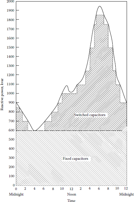
The remaining kilovar demands of the loads are met by the generator or preferably by the switched capacitors. However, since meeting the kilovar demands of the system from the generator is too expensive and may create problems in the system stability, capacitors are used. Capacitor sizes are selected to match the remaining load characteristics from hour to hour.
Many utilities apply the following rule of thumb to determine the size of the switched capacitors: Add switched capacitors until
From the voltage regulation point of view, the kilovars needed to raise the voltage at the end of the feeder to the maximum allowable voltage level at minimum load (25% of peak load) are the size of the fixed capacitors that should be used. On the other hand, if more than one capacitor bank is installed, the size of each capacitor bank at each location should have the same proportion, that is,
However, the resultant voltage rise must not exceed the light-load voltage drop. The approximate value of the percent voltage rise can be calculated from
where
%VR is the percent voltage rise
Qc,3ϕ is the three-phase reactive power due to fixed capacitors applied, kvar x is the line reactance, O/min
l is the length of feeder from sending end of feeder to fixed capacitor location, min
VL–L is the line-to-line voltage, kV
The percent voltage rise can also be found from
where
If the fixed capacitors are applied to the end of the feeder and if the percent voltage rise is already determined, the maximum value of the fixed capacitors can be determined from
Equations 8.31 and 8.32 can also be used to calculate the percent voltage rise due to the switched capacitors. Therefore, once the percent voltage rises due to both fixed and switched capacitors, the total percent voltage rise can be calculated as
where
is the total percent voltage rise
%VRNSW is the percent voltage rise due to fixed (or nonswitched) capacitors
%VRSW is the percent voltage rise due to switched capacitors
Some utilities use the following rule of thumb: The total amount of fixed and switched capacitors for a feeder is the amount necessary to raise the receiving-end feeder voltage to maximum at 50% of the peak feeder load.
Once the kilovars of capacitors necessary for the system are determined, there remains only the question of proper location. The rule of thumb for locating the fixed capacitors on feeders with uniformly distributed loads is to locate them approximately at two-thirds of the distance from the substation to the end of the feeder.
For the uniformly decreasing loads, fixed capacitors are located approximately halfway out on the feeder. On the other hand, the location of the switched capacitors is basically determined by the voltage regulation requirements, and it usually turns out to be the last one-third of the feeder away from the source.
8.5.2 Types of Controls for Switched Shunt Capacitors
The switching process of capacitors can be done by manual control or by automatic control using some type of control intelligence. Manual control (at the location or as remote control) can be employed at distribution substations. The intelligence types that can be used in automatic control include time–switch, voltage, current, voltage–time, voltage–current, and temperature.
The most popular types are the time-switch control, voltage control, and voltage––current control. The time–switch control is the least–expensive one. Some combinations of these controls are also used to follow the reactive load–duration curve more closely, as illustrated in Figure 8.20.

Meeting the reactive power requirements with fixed, voltage-controlled, and time-controlled capacitors.
8.5.3 Types of Three-Phase Capacitor-Bank Connections
A three-phase capacitor bank on a distribution feeder can be connected in (1) delta, (2) grounded wye, or (3) ungrounded wye. The type of connection used depends upon the following:
- System type, that is, whether it is a grounded or an ungrounded system
- Fusing requirements
- Capacitor-bank location
- Telephone interference considerations
A resonance condition may occur in delta and ungrounded-wye (floating neutral) banks when there is a one- or two-line open-type fault that occurs on the source side of the capacitor bank due to the maintained voltage on the open phase that backfeeds any transformers located on the load side of the open conductor through the series capacitor. As a result of this condition, the singlephase distribution transformers on four-wire systems may be damaged. Therefore, ungrounded-wye capacitor banks are not recommended under the following conditions:
- On feeders with light load where the minimum load per phase beyond the capacitor bank does not exceed 150% of the per phase rating of the capacitor bank
- On feeders with single-phase breaker operation at the sending end
- On fixed capacitor banks
- On feeder sections beyond a sectionalizing-fuse or single-phase recloser
- On feeders with emergency load transfers
However, the ungrounded-wye capacitor banks are recommended if one or more of the following conditions exist:
- Excessive harmonic currents in the substation neutral can be precluded.
- Telephone interferences can be minimized.
- Capacitor-bank installation can be made with two single-phase switches rather than with three single-pole switches.
Usually, grounded-wye capacitor banks are used only on four-wire three-phase primary systems. Otherwise, if a grounded-wye capacitor bank is used on a three-phase three-wire ungrounded-wye or delta system, it furnishes a ground current source that may disturb sensitive ground relays.
8.6 Economic Justification for Capacitors
Loads on electric utility systems include two components: active power (measured in kilowatts) and reactive power (measured in kilovars). Active power has to be generated at power plants, whereas reactive power can be provided by either power plants or capacitors. It is a well-known fact that shunt power capacitors are the most economical source to meet the reactive power requirements of inductive loads and transmission lines operating at a lagging power factor.
When reactive power is provided only by power plants, each system component (i.e., generators, transformers, transmission and distribution lines, switchgear, and protective equipment) has to be increased in size accordingly. Capacitors can mitigate these conditions by decreasing the reactive power demand all the way back to the generators. Line currents are reduced from capacitor locations all the way back to generation equipment. As a result, losses and loadings are reduced in distribution lines, substation transformers, and transmission lines.
Depending upon the uncorrected power factor of the system, the installation of capacitors can increase generator and substation capability for additional load at least 30% and can increase individual circuit capability, from the voltage regulation point of view, approximately 30%–100%.
Furthermore, the current reduction in transformer and distribution equipment and lines reduces the load on these kilovoltampere-limited apparatus and consequently delays the new facility installations. In general, the economic benefits force capacitor banks to be installed on the primary distribution system rather than on the secondary.
It is a well-known rule of thumb that the optimum amount of capacitor kilovars to employ is always the amount at which the economic benefits obtained from the addition of the last kilovar exactly equal the installed cost of the kilovars of capacitors.
The methods used by the utilities to determine the economic benefits derived from the installation of capacitors vary from company to company, but the determination of the total installed cost of a kilovar of capacitors is easy and straightforward.
In general, the economic benefits that can be derived from capacitor installation can be summarized as follows:
- Released generation capacity
- Released transmission capacity
- Released distribution substation capacity
- Additional advantages in distribution system
- Reduced energy (copper) losses
- Reduced voltage drop and consequently improved voltage regulation
- Released capacity of feeder and associated apparatus
- Postponement or elimination of capital expenditure due to system improvements and/ or expansions
- Revenue increase due to voltage improvements
8.6.1 Benefits Due to Released Generation Capacity
The released generation capacity due to the installation of capacitors can be calculated approximately from
where
ΔSG is the released generation capacity beyond maximum generation capacity at original power factor, kVA
SG is the generation capacity, kVA
Qc is the reactive power due to corrective capacitors applied, kvar
cos θ is the original (or uncorrected or old) power factor before application of capacitors
Therefore, the annual benefits due to the released generation capacity can be expressed as
where
Δ$G is the annual benefits due to released generation capacity, $/year
ΔSG is the released generation capacity beyond maximum generation capacity at original power factor, kVA
CG is the cost of (peaking) generation, $/kW
iG is the annual fixed charge rate* applicable to generation
8.6.2 Benefits Due to Released Transmission Capacity
The released transmission capacity due to the installation of capacitors can be calculated approximately as
where
ΔST is the released transmission capacity† beyond maximum transmission capacity at original power factor, kVA
ST is the transmission capacity, kVA
Thus, the annual benefits due to the released transmission capacity can be found as
where
Δ$T is the annual benefits due to released transmission capacity, $/year
ΔST is the released transmission capacity beyond maximum transmission capacity at original power factor, kVA
CT is the cost of transmission line and associated apparatus, $/kVA
iT is the annual fixed charge rate applicable to transmission
8.6.3 Benefits Due to Released Distribution Substation Capacity
The released distribution substation capacity due to the installation of capacitors can be found approximately from
where
ΔSS is the released distribution substation capacity beyond maximum substation capacity at original power factor, kVA
SS is the distribution substation capacity, kVA
Hence, the annual benefits due to the released substation capacity can be calculated as
where
Δ$S is the annual benefits due to the released substation capacity, $/year
ΔSS is the released substation capacity, kVA
CS is the cost of substation and associated apparatus, $/kVA
iS is the annual fixed charge rate applicable to substation
8.6.4 Benefits Due to Reduced Energy Losses
The annual energy losses are reduced as a result of decreasing copper losses due to the installation of capacitors. The conserved energy can be expressed as
where
ΔACE is the annual conserved energy, kWh/year
Qc,3ϕ is the three-phase reactive power due to corrective capacitors applied, kvar
R is the total line resistance to load center, O
QL,3ϕ is the original, that is, uncorrected, three-phase load, kVA
sin θ is the sine of original (uncorrected) power factor angle
VL–L is the line-to-line voltage, kV
Therefore, the annual benefits due to the conserved energy can be calculated as
where
ΔACE is the annual benefits due to conserved energy, $/year
EC is the cost of energy, $/kWh
8.6.5 Benefits Due to Reduced Voltage Drops
The following advantages can be obtained by the installation of capacitors into a circuit:
- The effective line current is reduced, and consequently, both IR and IXL voltage drops are decreased, which results in improved voltage regulation.
- The power factor improvement further decreases the effect of reactive line voltage drop.
The percent voltage drop that occurs in a given circuit can be expressed as
where
%VD is the percent voltage drop
SL,3ϕ is the three-phase load, kVA
r is the line resistance, 0/min
x is the line reactance, 0/min
l is the length of conductors, min
VL-L is the line-to-line voltage, kV
The voltage drop that can be calculated from Equation 8.44 is the basis for the application of the capacitors. After the application of the capacitors, the system yields a voltage rise due to the improved power factor and the reduced effective line current. Therefore, the voltage drops due to IR and IXL are minimized. The approximate value of the percent voltage rise along the line can be calculated as
Furthermore, an additional voltage-rise phenomenon through every transformer from the generating source to the capacitors occurs due to the application of capacitors. It is independent of load and power factor of the line and can be expressed as
where
%VRT is the percent voltage rise through the transformer
ST,3ϕ is the total three-phase transformer rating, kVA
xT is the percent transformer reactance (approximately equal to the transformer’s nameplate impedance).
8.6.6 Benefits Due to Released Feeder Capacity
In general, feeder capacity is restricted by allowable voltage drop rather than by thermal limitations (as seen in Chapter 4). Therefore, the installation of capacitors decreases the voltage drop and consequently increases the feeder capacity.
Without including the released regulator or substation capacity, this additional feeder capacity can be calculated as
Therefore, the annual benefits due to the released feeder capacity can be calculated as
where
Δ$F is the annual benefits due to released feeder capacity, $/year
ΔSF is the released feeder capacity, kVA
CF is the cost of installed feeder, $/kVA
iF is the annual fixed charge rate applicable to the feeder
8.6.7 Financial Benefits Due to Voltage Improvement
The revenues to the utility are increased as a result of increased kilowatthour energy consumption due to the voltage rise produced on a system by the addition of the corrective capacitor banks. This is especially true for residential feeders.
The increased energy consumption depends on the nature of the apparatus used. For example, energy consumption for lighting increases as the square of the voltage used. As an example, Table 8.3 gives the additional kilowatthour energy increase (in percent) as a function of the ratio of the average voltage after the addition of capacitors to the average voltage before the addition of capacitors (based on a typical load diversity).
Additional kWh Energy Increase After capacitor addition
|
ΔkWh Increase, % |
|---|---|
1.00 | 0 |
1.05 | 8 |
1.10 | 16 |
1.15 | 25 |
1.20 | 34 |
1.25 | 43 |
1.30 | 52 |
Thus, the increase in revenues due to the increased kilowatthour energy consumption can be calculated as
where
Δ$BEC is the additional annual revenue due to increased kWh energy consumption, $/year
ΔBEC is the additional kWh energy consumption increase
BEC is the original (or base) annual kWh energy consumption, kWh/year
8.6.8 Total Financial Benefits Due to Capacitor Installations
Therefore, the total benefits due to the installation of capacitor banks can be summarized as
The total benefits obtained from Equation 8.50 should be compared against the annual equivalent of the total cost of the installed capacitor banks. The total cost of the installed capacitor banks can be found from
where
ΔEICc is the annual equivalent of the total cost of installed capacitor banks, $/year
ΔQc is the required amount of capacitor-bank additions, kvar
ICc is the cost of installed capacitor banks, $/kvar
ic is the annual fixed charge rate applicable to capacitors
In summary, capacitors can provide the utility industry with a very effective cost reduction instrument. With plant costs and fuel costs continually increasing, electric utilities benefit whenever new plant investment can be deferred or eliminated and energy requirements reduced.
Thus, capacitors aid in minimizing operating expenses and allow the utilities to serve new loads and customers with a minimum system investment. Today, utilities in the United States have approximately 1 kvar of power capacitors installed for every 2 kW of installed generation capacity in order to take advantage of the economic benefits involved [4].
Example 8.19*
Assume that a large power pool is presently operating at 90% power factor. It is desired to improve the power factor to 98%. To improve the power factor to 98%, a number of load flow runs are made, and the results are summarized in Table 8.4.
For Example 8.19
Comment |
At 90% PF |
At 98% PF |
|---|---|---|
Total loss reduction due to capacitors applied to substation buses, kW |
495,165 |
491,738 |
Additional loss reduction due to capacitors applied to feeders, kW |
85,771 |
75,342 |
Total demand reduction due to capacitors applied to substation buses and feeders, kVA |
22,506,007 |
21,172,616 |
Total required capacitor additions at buses and feeders, kvar |
9,810,141 |
4,213,297 |
Assume that the average fixed charge rate is 0.20, average demand cost is $250/kW, energy cost is $0.045/kWh, the system loss factor is 0.17, and an average capacitor cost is $4.75/kvar. Use responsibility factors of 1.0 and 0.9 for capacitors installed on the substation buses and on feeders, respectively. Determine the following:
- The resulting additional savings in kilowatt losses at the 98% power factor when all capacitors are applied to substation buses.
- The resulting additional savings in kilowatt losses at the 98% power factor when some capacitors are applied to feeders.
- The total additional savings in kilowatt losses.
- The additional savings in the system kilovoltampere capacity.
- The additional capacitors required, kvars.
- The total annual savings in demand reduction due to additional capacitors applied to substation buses and feeders, $/year.
- The annual savings due to the additional released transmission capacity, $/year.
- The total annual savings due to the energy loss reduction, $/year.
- The total annual cost of the additional capacitors, $/year.
- The total net annual savings, $/year.
- Is the 98% power factor the economic power factor?
Solution
- From Table 8.4, the resulting additional savings in kilowatt losses due to the power factor improvement at the substation buses is
- From Table 8.4 for feeders,
- Therefore, the total additional kilowatt savings is
As can be observed, the additional kilowatt savings due to capacitors applied to the feeders is more than three times that of capacitors applied to the substation buses. This is due to the fact that power losses are larger at the lower voltages.
- From Table 8.4, the additional savings in the system kilovoltampere capacity is
- From Table 8.4, the additional capacitors required are
- The annual savings in demand reduction due to capacitors applied to distribution substation buses is approximately
and due to capacitors applied to feeders is
Therefore, the total annual savings in demand reduction is
- The annual savings due to the additional released transmission capacity is
- The total annual savings due to the energy loss reduction is
- The total annual cost of the additional capacitors is
- The total annual savings is summation of the savings in demand, capacity, and energy:
Therefore, the total net annual savings is
- No, since the total net annual savings is not zero.
8.7 Practical Procedure to Determine the Best Capacitor Location
In general, the best location for capacitors can be found by optimizing power loss and voltage regulation. A feeder voltage profile study is performed to warrant the most effective location for capacitors and the determination of a voltage that is within recommended limits.
Usually, a 2 V rise on circuits used in urban areas and a 3 V rise on circuits used in rural areas are approximately the maximum voltage changes that are allowed when a switched capacitor bank is placed into operation. The general iteration process involved is summarized in the following steps:
- Collect the following circuit and load information:
- Any two of the following for each load: kilovoltamperes, kilovars, kilowatts, and load power factor
- Desired corrected power of circuit
- Feeder-circuit voltage
- A feeder-circuit map that shows locations of loads and presently existing capacitor banks
- Determine the kilowatt load of the feeder and the power factor.
- From Table 8.2, determine the kilovars per kilowatts of load (i.e., the correction factor) necessary to correct the feeder-circuit power factor from the original to the desired power factor. To determine the kilovars of capacitors required, multiply this correction factor by the total kilowatts of the feeder circuit.
- Determine the individual kilovoltamperes and power factor for each load or group of loads.
- To determine the kilovars on the line, multiply individual load or groups of loads by their respective reactive factors that can be found from Table 8.2.
- Develop a nomograph to determine the line loss in W/1000 ft due to the inductive loads tabulated in steps 4 and 5. Multiply these line losses by their respective line lengths in thousands of feet. Repeat this process for all loads and line sections and add them to find the total inductive line loss.
- In the case of having presently existing capacitors on the feeder, perform the same calculations as in step 6, but this time subtract the capacitive line loss from the total inductive line loss. Use the capacitor kilovars determined in step 3 and the nomograph developed for step 6 and find the line loss in each line section due to capacitors.
- To find the distance to capacitor location, divide the total inductive line loss by capacitive line loss per thousand feet. If this quotient is greater than the line section length
- Divide the remaining inductive line loss by the capacitive line loss in the next line section to find the location
- If this quotient is still greater than the line section length, repeat step 8a
- Prepare a voltage profile by hand calculations or by using a computer program for voltage profile and load analysis to determine the circuit voltages. If the profile shows that the voltages are inside the recommended limits, then the capacitors are installed at the location of minimum loss. If not, then use engineering judgment to locate them for the most effective voltage control application.