10.12 Fault-Current Calculations in Per Units
Fault currents can also be determined by using per unit values rather than actual system values, of course. For example, Anderson [3] gives fault-current formulas that use per unit values, as shown in Table 10.12.
Fault-Current Formulas in Per Unit
Fault Type |
Fault-Current Formula |
Source Connection |
|---|---|---|
3ϕ |
ˉIf,3ϕ=ˉVfˉZsys+ˉZT+ˉZckt+ˉZf |
Delta or grounded wye |
L-L |
ˉIf,b=−ˉIf,c=−j√3×ˉVf2(ˉZsys+ˉZT+ˉZckt)+ˉZf |
Delta or grounded wye |
L-G |
ˉIf,a=0 |
Delta or |
ˉIf,a=3ˉVf2ˉZsys+3ˉZT+6ˉZckt+3ˉZf |
Grounded wyea |
Source: Anderson, P.M., Elements of Power System Protection, Cyclone Copy Center, Ames, IA, 1975.
a Using K0 = 4, from Table 10.6.
Example 10.3
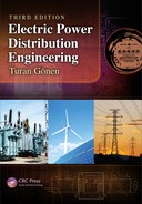
Assume that a distribution substation, shown in Figure 10.31, has a 5000 kVA 69/12.47 kV LTC transformer feeding a three-phase four-wire 12.47 kV distribution system. The transformer has a reactance of 0.065 pu Ω. Assume that the faults are bolted with zero fault impedance and that the maximum and minimum power generations of the system are 600 and 360 MVA, respectively. Use 1 MVA as the three-phase power base:
- Under the maximum (system) power generation conditions, determine the available three-phase, L-L, and SLG fault currents at buses 1 and 2 in per units, in amperes, and in megavoltamperes.
- Under the minimum (system) power generation conditions, determine the available three-phase, L-L, and SLG fault currents at buses 1 and 2 in per units, in amperes, and in megavoltamperes.
- Tabulate the results obtained in parts a and b.
- Selecting 69 kV as the voltage base, the impedance base can be determined as
ZB=V2B,L−LSB,3ϕ=(69×103)21×106=4761 Ω
Therefore, under the maximum (system) power generation conditions, the system impedance is
Zsys=(69×103)2600×106=7.935 Ω
or
Zsys=7.9354761=0.0017 pu Ω
Similarly, the three-phase current base can be found as
IB=SB,3ϕ√3×VB,L−L=1×10⁶√3(69×103)=8.3674 A
- i. At bus 1, from Table 10.12, the three-phase fault current can be calculated as
ˉIf,3ϕ=|ˉVfˉZsys+ˉZT+ˉZckt+ˉZf|=|1.0j0.0017+0+0+0|≅588.2 pu A
(note that it is assumed that the voltage is 1.0 pu V at the fault point.)
or
If,3ϕ=(588.2 pu A)(8.3674 A)=4922 A
or
Sf,3ϕ=√3(69 kV)(4922)×10−3≅588.2 MVA
The L-L fault current can be calculated by using the appropriate equation from Table 10.12 or from
If,L−L=0.8666If,3ϕ=0.866(588.2 pu A)≅509.38 pu A=4262.5 A
or
Sf,L−L=(69 kV)(4267.2 A)10−3=294.1 MVA
From Table 10.12, the SLG fault current can be calculated as or
If,L−L=3ˉVf2ˉZsys+3ˉZT+6ˉZckt+3ˉZf=|3(1.0)2(j0.0017)+0+0+0|=882.35 pu A=7383 A
or
Sf,L−G=(69 kV√3)(7383 A) 10−3=294.1 MVA
- ii. At bus 2, since the given transformer reactance of 0.065 pu Ω value is based on 5 MVA, it has to be converted to the new base of 1 MVA. Therefore,
ZT,new=ZT,old(VB,L−L,oldVB,L−L,new)2SB,3ϕ,newSB,3ϕ,old=j0.065(69 kV69 kV)21MVA5MVA=j0.013 pu Ω=ZB=(12.47 × 10³)21×106=155.5Ω=IB=1×10⁶√3(12.47×10³)=46.2991 A
Thus,
If,3ϕ=|1.0j0.0017+j0.013+0+0|=68.0272 pu A
or
If,3ϕ=(68.0272pu A)(46.2991A)≅3149.6A
or
Sf,3ϕ=√3(12.47 kV)(3149.6)10−3=68.0272 MVA
If,L−L=0.866(If,3ϕ)=0.866(68.0272 pu A)=58.9116 pu A=2727.6 A
or
Sf,L−L=(12.47 kV)(2727.6 A)10−3=34.01 MVA
If,L−G=|3(1.0)2(j0.0017)+3(j0.013)+0+0|=70.7547 pu A≅3275.9 A
Sf,L−G=(12.47 kV√3)(3275.9 A)10−3≅23.58 MVA
- i. At bus 1, from Table 10.12, the three-phase fault current can be calculated as
- Under the minimum (system) power generation conditions, the system impedance becomes
Zsys=(69×103)2360×106=13.225 Ω
or
Zsys=13.2254761=j0.0028 pu Ω
- i At bus 1,
If,3ϕ=|1.0j0.0028+0+0+0|=360 pu A=3012.3 A
or
Sf,3ϕ=√3(69 kV)(3012.3 A)10-3=360 MVAIf,L−L=0.866 × If,3ϕ=311.76pu A=2608.7 A
or
Sf,L−L=(69kV)(2608.7 A)10-3≅180.2 MVA
If,L−G=|3(1.0)2(j0.0028)+0+0+0|=535.7 pu A=4482.5 A
or
If,L−G=(69kV√3)(4487.8 A)10-3≅178.6MVA
- ii. At bus 2,
If,3ϕ=|1.0j0.0028+j0.013+0+0|=63.2911 pu A≅2930.3 A
or
Sf,3ϕ=(12.47 kV)(2933.8 A)10-3≅63.29 MVA
If,L−L=0.866 × If,3ϕ=54.81 pu A≅2537.7 A
or
Sf,L−L=(12.47 kV)(2540.7 A)10-3≅36.6 MVA
If,L−G=|3(1.0)2(j0.0028)+3(j0.013)+0+0|=67.2646 pu A≅3114.3 A
or
Sf,L−G=(12.47 kV√3)(3114.3 A)10−3≅22.42 MVA
- i At bus 1,
- The results are given in Table 10.13.
Results of Example 10.3
Maximum Generation |
Minimum Generation |
||||
|---|---|---|---|---|---|
BUS |
Fault |
A |
MVA |
A |
MVA |
1 |
3ϕ |
4922 |
588.2 |
3012.3 |
360 |
L-L |
4266.5 |
294.1 |
2608.7 |
180.2 | |
L-G |
7383 |
294.1 |
4482.5 |
178.6 | |
2 |
3ϕ |
3149.6 |
68.0 |
2930.3 |
63.29 |
L-L |
2727.6 |
34.0 |
2537.7 |
36.6 | |
L-G |
3275.9 |
23.6 |
3114.3 |
23.42 | |
10.13 Secondary-System Fault-Current Calculations
10.13.1 Single-Phase 120/240 V Three-Wire Secondary Service
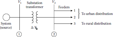
As shown in Figure 10.32, a line-to-ground fault may involve line l1 and neutral or line 12 and neutral. Therefore, the maximum line-to-ground fault current can be calculated as
ˉIf,L−G=ˉVL−NˉZeq(10.46)
or
ˉIf,L−G=0.5ˉVL−LˉZeq(10.47)
where
ˉZeq=ˉZT+n2ˉZG+ˉZG,SL(10.48)
is the equivalent impedance to fault, Ω
ˉZT is the equivalent impedance of distribution transformer,* Ω
=1.5RT+j1.2XT(10.49)
ˉZG is the line-to-ground impedance of primary system, Ω
ˉZG,SL is the line-to-ground impedance of secondary line, Ω
n is the primary-to-secondary impedance-transfer ratio †
=sec VL−Npri VL−N(10.50)
Also, maximum L-L fault may occur between lines l1 and l2. Therefore,
ˉIf,L−N= ˉVL−N ˉZL−N(10.51)
where
ˉZeq=ˉZT+n2ˉZG+ˉZ1,SL(10.52)
ˉZT is the equivalent impedance of distribution transformer, Ω
=Z(10.53)
ˉZ1,SL is the positive-sequence impedance of secondary line, Ω
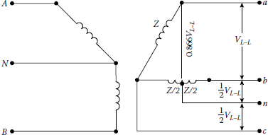
10.13.2 Three-Phase 240/120 or 480/240 V Wye–Delta or Delta–Delta Four-Wire Secondary Service
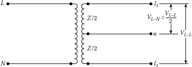
For a delta-connected secondary, if the primary is connected in wye, its impedance must be converted to its equivalent delta impedance, as indicated in Figure 10.33. Therefore,
A wye–delta or delta–delta secondary service. If needed, the wye primary can be replaced with its equivalent delta, as illustrated.
ˉZΔ=ˉZ1ˉZ1+ˉZ1ˉZ1+ˉZ1ˉZ1ˉZ1=3ˉZ1(10.54)
where
ˉZ1 is the positive-sequence impedance, Ω
ˉZΔ is the equivalent delta impedance, Ω
If the primary is already connected in delta, then
ˉZΔ=ˉZ1(10.55)
As shown in Figure 10.33, a line-to-ground fault may involve phase a and neutral. The resultant maximum line-to-ground fault current can be expressed as
ˉIf,L−G=0.866×ˉVL−LˉZeq(10.56)
where
ˉZeq=ˉZT+n2ˉZΔ+ˉZG,SL(10.57)
ˉZT=(ˉZ+ˉZ/2)(ˉZ+ˉZ/2)2(ˉZ+(ˉZ/2))=3ˉZ4(10.58)
If the line-to-ground fault involves phase b and neutral or phase c and neutral, then the maximum available line-to-ground fault current can be calculated as
ˉIf,L−G=0.5×ˉVL−LˉZeq(10.59)
where ˉZeq is found from Equation 10.57 and
ˉZT=ˉZ/2(2ˉZ+ˉZ/2)2(ˉZ+(ˉZ/2))=5ˉZ12(10.60)
An L–L fault may involve phases a and b, or b and c, or c and a. In any case, the maximum L-L fault current can be calculated from Equation 10.51 where
ˉZeq=ˉZT+n2ˉZΔ+ˉZ1,SL(10.61)
and
ˉZT=(2ˉZ)(ˉZ)2ˉZ+ˉZ=2ˉZ3(10.62)
A three-phase fault, of course, involves all three phases. Therefore,
ˉIf,3ϕ=ˉVL−L√3×ˉZeq(10.63)
where
Zeq=ZT+n2ZΔ+Z1,cable(10.64)
ˉZT=ˉZ(10.65)
10.13.3 Three-Phase 240/120 or 480/240 V Open-Wye Primary and Four-Wire Open-Delta Secondary Service
Figure 10.34 shows a three-phase open-wye primary and four-wire open-delta secondary connection. If a line-to-ground fault involves phase b and neutral or phase c and neutral, the maximum available fault current can be calculated as
ˉIf,L−G=0.5×ˉVL−LˉZeq(10.66)
where
ˉZeq is found from Equation 10.48
n is the transfer ratio found from Figure 10.35a
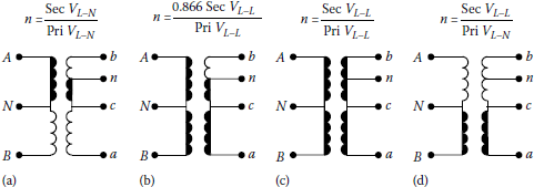
Various fault-current paths in the transformer and associated impedance-transfer ratios.
(The shaded path determines the primaryand secondary-transformer fault impedances.)
If the line-to-ground fault involves phase a and neutral, the maximum available fault current can be expressed as
ˉIf,L−G=0.886×ˉVL−LˉZeq(10.67)
where
ˉZeq=ˉZT+n2ˉZ1+ˉZG,SL(10.68)
n is the transfer ratio from Figure 10.35b
ˉZT=ˉZ+ˉZ2=(RT+1.5RT)+j(XT+1.2XT)(10.69)
If an L–L fault involves phases a and b, the available fault current can be calculated from Equation 10.51, where
ˉZeq=ˉZT+n2ˉZ1+ˉZ1,SL(10.70)
n is the transfer ratio from Figure 10.35c
ˉZT=2ˉZ(10.71)
If an L–L fault involves phases a and c or phases b and c, the available fault current can be calculated by using Equations 10.51 and 10.52, where
n is the transfer ratio from Figure 10.35d
ˉZT=ˉZ
Since a three-phase fault involves all three phases, the maximum three-phase fault current can be determined from
ˉIf,3ϕ=ˉVL−LˉZeq(10.72)
where ˉZeq is found from Equation 10.70 and
ˉZT=(3ˉZ)(3ˉZ)6ˉZ=3ˉZ2(10.73)
10.13.4 Three-Phase 208Y/120 V, 480Y/277 V, or 832Y/480 V Four-Wire Wye-Wye Secondary Service
Figure 10.36 shows a three-phase wye–wye–connected four-wire secondary connection. A line-toground fault may involve any one of the three phases and neutral. The maximum line-to-ground fault current can be calculated as
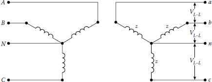
ˉIf,L−G=ˉVL−NˉZeq(10.74)
where is found from Equation 10.48 and
An L–L fault may involve phases a and b, or b and c, or c and a. The available L–L fault current is
where is determined from Equation 10.70 and
A three-phase fault may involve all three phases; therefore, the available three-phase fault current can be expressed as
where is determined from Equation 10.70.
Example 10.4
Assume that there is a single-phase L–L secondary fault on a 120/240 V three-wire service, as shown in Figure 10.37, and that the subtransmission system is taken as an infinite bus. The substation transformer is a three-phase 7500 kVA with 7% impedance and 1% resistance. The 12.47 kV primary feeder has three-phase conductors of 336AS37 with a neutral conductor of 0AS7 at 62 in. spacing.
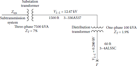
The secondary transformer (i.e., distribution transformer) has 100 kVA capacity with 1.9% impedance and 1% resistance. The 60 ft long self-supporting service cable (SSC) with ACSR neutral has three wires and is given to be 3-4ALSSC. Assume that it has a resistance of 0.4660 Ω/1000 ft and a reactance of 0.0293 Ω/1000 ft. Use Table 10.7 to determine the necessary sequenceimpedance values for the primary line and determine the following:
- The impedance of the substation transformer, Ω
- The positive- and zero-sequence impedance of the line, Ω
- The line-to-ground impedance in the primary system, Ω
- The total impedance through the primary, Ω
- The total primary impedance referred to secondary, Ω
- The distribution transformer impedance, Ω
- The impedance of the secondary cable, Ω
- The total impedance to the fault, Ω
- The single-phase L–L fault for the 120/240 V three-wire service, A
Solution
- Since the impedance of the substation transformer can be expressed as
where its reactance is
and
therefore
- From Table 10.7, the positive-sequence impedance of the primary line is
and similarly the zero-sequence impedance is
- From Equation 10.17,
- Since the subtransmission system is assumed to be an infinite bus,
therefore the total impedance through the primary is
- From Equation 10.50, the total primary impedance referred to secondary is
- The secondary (i.e., distribution) transformer reactance can be determined as
Therefore, its impedance can be expressed as or
or
- Since the impedance of the secondary cable is given in Ω/1000 ft, for a 60 ft length,
- Therefore, the total impedance to the fault can be found as
- Thus, from Equation 10.51, the fault current at the secondary fault point F is
10.14 High-Impedance Faults
The detection of high-impedance faults on electric distribution systems has been one of the most difficult and persistent problems. These faults result from the contact of an energized conductor with surfaces or objects that limit the current to levels below the detection thresholds of conventional protection devices. High-impedance faults often take place when an energized overhead conductor breaks and falls to the ground, creating a serious public hazard.
The typical measured values of primary fault current for a 15 kV class of distribution feeder conductor in contact with various surfaces are 0 A for dry asphalt or sand, 15 A for wet grass, 20 A for dry sod, 25 A for dry grass, 40 A for wet sod, 50 A for wet grass, and 75 A for reinforced concrete. Recent advances in digital technology have provided a means of detecting most of these previously undetectable faults.
However, it is still impossible to detect all high-impedance faults, because of the random and intermittent nature of these low current faults. For example, in one of the methods, an electromechanical time-overcurrent relay, which balanced zero-sequence operating torque against positive- and negative-sequence bias, showed an increased sensitivity but with disappointing security. Also, several mechanical devices have been developed to catch and ground a broken conductor, but they appear to have questionable reliability and are costly. They are also difficult to install.
The single most important measure that might be taken, in any power system and without product expense, to improve system protection against arcing faults would be to lower circuit-breaker instantaneous trip settings to a level no higher than that required to avoid nuisance tripping under normal conditions. Because of the inadequacies of fuses and arcing-fault currents, recourse to supplementary relaying is necessary to secure adequate protection.
Both grounded and ungrounded systems have proven valuable to arcing-fault burndowns. The ungrounded power system tends to present higher probable minimum values of arcing-fault current under certain conditions, when compared to the grounded system. The ungrounded system can have substantial transient overvoltages in the event of faults [16].
Ground fault currents in a system, which is solidly grounded, may have values approaching or exceeding the bolted three-phase short-circuit values, and automatically and prompt interruption of circuits faulted to ground is the intended mode of operation.
The solidly grounded system is the most widely used low-voltage distribution system, in either the industrial or commercial building domain. The ideal solution to the problem would be sensitive to arcing-fault current alone. Since arcing faults in grounded systems almost invariably involve ground, this fat permits a near-perfect approach to the ideal solution.
An excellent method of monitoring the presence of ground fault currents (zero-sequence currents) is provided by the use of a window or doughnut-type CT in combination with an overcurrent relay. All the phase conductors of the circuit to be monitored (plus the neutral conductor, if used) are passed through the window of the CT. With this arrangement (a low-voltage ground-sensor relay combination), only circuit faults involving ground will produce a current in the CT secondary to pick up the relay. By proper matching of the CT and relay, this arrangement may be made quite sensitive, so as to operate on ground currents of 15 A or less.
In the early 1980s, researchers [14] were focused on using an integrated multialgorithm approach in solving this nagging problem. The resultant partial success was due to the following developments in the digital technology: (1) rapid increase in digital processing power, (2) emergence of artificial intelligence methodology, and (3) advances in pattern recognition techniques. The random intermittent nature of these arcing faults required extensive data capture over relatively long-term intervals. Analysis of this expanding database enabled the researchers distinguish high-impedance faults from other power system events. This pattern recognition approach provided the basis for the development of the high-impedance fault detection algorithms.
One of the main algorithms is based on the recognition of sudden and sustained changes in energy in the extracted nonharmonic, as well as the harmonic components, of the feeder CT secondary currents. A second algorithm identifies the distinctive random changes in these extracted signals. In addition to the energy and randomness algorithms, various other algorithms address such things as spectral shape and arc burst patterns to further confirm the presence of arcing high-impedance faults.
While no one of these detection algorithms conclusively distinguishes all types of arcing faults from power system operational events, the integration of all of these algorithms into a knowledgebased system provides sensitive, reliable detection with excellent security. This expert arc-detection system requires a large amount of signal processing in real time during a fault or disturbance to run the various algorithms. Additional intelligence is provided to determine whether a high-impedance fault condition involves a primary conductor on the ground [14–16].
10.15 Lightning Protection
Momentary outages are a main concern for some utilities trying to improve their power quality. Improving protection of overhead distribution circuits from lightning is one way in which some utilities can significantly reduce the number of momentary outages. In most cases, flashovers result in a flash. The fault can be cleared by the substation breaker on the instantaneous setting of the relay, and the system will be back to normal following reclosure. This causes a momentary outage for the entire feeder that, in the past, may not have been a problem. However, modern consumer devices (such as digital clocks, computers, and VCRs) are disrupted by momentary outages, so many utilities are looking for ways to reduce those interruptions.
The voltages by nearby strokes are determined in a similar manner as the method used for direct strokes. For the direct stroke calculations, a current surge is injected into the conductor, and the traveling wave calculations are done. The induced voltage calculations are more complex but are similar in that they use the same traveling wave calculation method. The main difference is that currents are induced at each point along the line instead of a current injected at one point.
The electromagnetic fields created by the lightning stroke induce voltages and currents all along the line, but they can all be computed by considering the fields acting on very small conductor segments. Antenna theory is used to compute the electric and magnetic fields near the line segments due to the current stroke some distance away. Digital analysis becomes necessary due to the complexities involved with multiple phases, arresters, and ground impedances.
10.15.1 A Brief Review of Lightning Phenomenon
By definition, lightning is an electric discharge. It is the high-current discharge of an electrostatic electricity accumulation between the cloud and earth or between the clouds. The mechanism by which a cloud becomes electrically charged is not yet fully understood.
However, it is known that the ice crystals in an active cloud are positively charged, while the water droplets usually carry negative charges. Therefore, a thundercloud has a positive center in its upper section and a negative charge center in its lower section. Electrically speaking, this constitutes dipole. Note that the charge separation is related to the supercooling and occasionally even the freezing of droplets. The disposition of charge concentrations is partially due to the vertical circulation in terms of updrafts and downdrafts.
As a negative charge builds up in the cloud base, a corresponding positive charge is induced on earth, as shown in Figure 10.38a. The voltage gradient in the air between charge centers in cloud (or clouds) or between cloud and earth is not uniform, but it is maximum where the charge concentration is greatest.
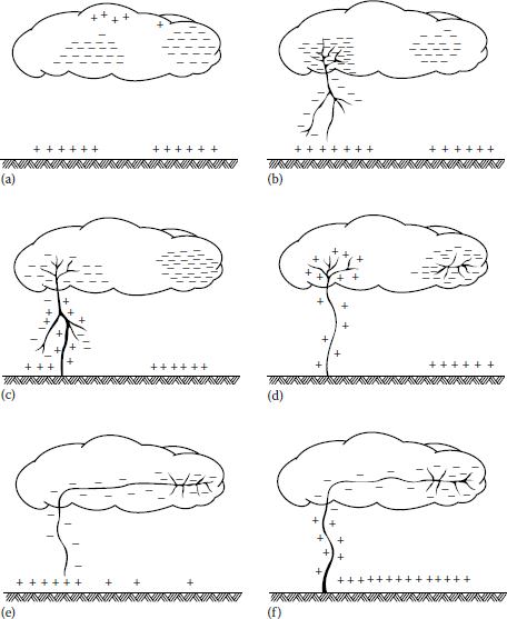
When voltage gradient within the cloud builds up to the order of 5–10 kV/cm, the air in the region breaks down and an ionized path called leader or leader stroke starts to form, moving from the cloud up to the earth, as shown in Figure 10.38b. The tip of the leader has a speed between 105 and 2 × 10⁵ m/s (i.e., less than 1000th of the speed of the light of 3 × 10⁸ m/s) and moves in jumps. If photographed by a camera lens of which is moving from left to right, the leader stroke would appear as shown in Figure 10.39. Therefore, the formation of a lightning stroke is a progressive breakdown of the arc path from the cloud to the earth.
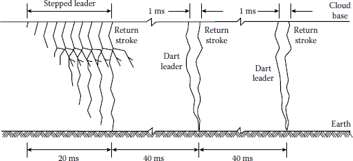
As the leader strikes the earth, an extremely bright return streamer, called return stroke, propagates upward from the earth to the cloud following the same path, as shown in Figures 10.38c and 10.39. In a sense, the return stroke establishes an electric short circuit between the negative charge deposited along the leader and the electrostatically induced positive charge on the ground.
Therefore, the charge energy from the cloud is related into the ground, neutralizing the charge centers. The initial speed of the return stroke is 108 m/s. The current involved in the return stroke has a peak value of from 1 to 200 kA, lasting about 100 μs. About 40 μs later, a second leader, called dart leader, may stroke usually following the same path taken by the first leader.
Dart leader is much faster and has no branches and may be produced by discharge between two charge centers in the cloud, as shown in Figure 10.38e. Note the distribution of the negative charge along the stroke path. The process of dart leader and return stroke (Figure 10.38f) can be repeated several times.
The complete process of successive strokes is called lightning flash. Thus, a lightning flash may have a single or a sequence of several discrete stokes (as many as 40) separated by about 40 ms, as shown in Figure 10.39.
10.15.2 Lightning Surges
The voltages produced on overhead lines by lightning may be due to indirect strokes or direct strokes. In the indirect stroke, induced charges can take place in the lines as a result of close-by lightning strokes to ground. Even though the cloud and earth charges are neutralized through the established cloud-to-earth current path, a charge will be trapped on the line, as shown in Figure 10.40a.
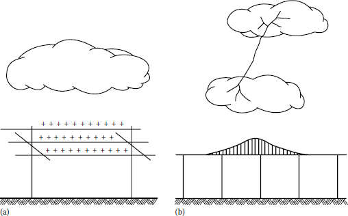
(a) Induced line charges due to indirect lightning strokes and (b) an occurence of a lightning among clouds.
The magnitude of this trapped charge is a function of the initial cloud-to-earth voltage gradient and the closeness of the stroke to the line. Such voltage may also be induced as a result of lightning among clouds, as shown in Figure 10.40. In any case, the voltage induced on the line propagates along the line as a traveling wave until it is dissipated by attenuation, leakage, insulation failure, or arrester operation.
A direct lightning can hit any point on a line. It can hit a pole or somewhere in the span between poles. If lightning hits a pole top, some of the current may flow through the shield wires if there is any, and the remaining current flows through the pole to the earth. The flashover will look like a fireball enveloping the top of the pole. The current will divide at the neutral connection, and a small part of it will travel down the line in both directions to the poles on each side of the struck pole.
When the two traveling lightning current waves reach the two adjacent grounded poles, the current will be traveling to these pole grounds, and a small part will continue down the line to the next pole grounds. In general, all of the current can be assumed to flow into the ground at the pole that is struck and the first two grounded poles adjacent to it. If the earth resistance is high, several more grounded poles may be involved on either side of the struck pole.
However, if lightning hits midspan on a distribution line, the lightning current will divide, and half will travel along the line in each direction at almost the speed of light. If the lightning current flowing through the surge impedance of the line produces a voltage greater than the line insulation can withstand, flashover will take place on the two poles adjacent to the strike point. In addition, strokes that terminate near the line but do not actually hit it can induce voltages high enough to cause flashovers.
To the voltage and current waves, the dead end will appear to be an open circuit. The current wave will be reflected back down the line with a reversed polarity. The voltage wave will double and be reflected back down the line with the same polarity.
Because of the low basic lightning impulse level (BIL) of distribution lines and the lightning peak-current magnitudes, voltage doubling at dead ends will produce flashover at all unprotected dead ends, resulting in a line outage. Most dead ends have installed surge arresters, which prevent voltage doubling. A surge arrester should be installed on all dead ends.
10.15.3 Lightning Protection
Shunting and shielding are two basic methods used to protect lines. With shunting method, lightning is permitted to strike the phase conductors, and the lightning current is shunted to ground either by a flashover or by lightning arresters.
With shielding, a separate conductor (called overhead ground wire) is installed above the phase conductors, and the lightning current is routed to ground without flowing through the phase conductors.
Shielding is used mostly on transmission lines. Shunting is used mainly on distribution lines. The shield wire intercepts the lightning strike. This is accomplished at distribution-line heights by using a 30° protective angle. (This is the angle between the vertical and a straight line between the shield wire and the outside phase conductor.) It is important that there is enough insulation between the phase conductors and the shield system to prevent flashover.
When lightning strikes the shield wire, it travels down the shield to the first structure and down the pole ground to earth. The flow of current in the pole ground results in a voltage between it and the phase conductors. If the insulation strength (i.e., BIL of the line) is exceeded by this voltage, flashover occurs.
Since the lightning current is flowing in the ground circuit instead of the phase conductor, the phenomenon is known as the backflash. On the other hand, when lightning strikes a line directly, the raised voltage, at the contact point, propagates in the form of a traveling wave in both directions and raises the potential of the line to the voltage of the downward leader.
If the line is not properly protected against such overvoltage, such voltage may exceed the lineto-ground withstand voltage of the line insulation failure, or preferably the arrester operation establishes a path from the line conductor to ground for the lightning surge current.
To achieve reasonable performance with a shield system on distribution lines, the BIL of the path between the insulators and the pole ground is required to be in the 500–600 kV range, and the pole ground impedance has to be less than 10 Ω. Also, every single pole is required to have a pole ground installed.
In general, the cost of a properly designed shield system will considerably exceed the cost of a lightning arrester-protected system. A lightning arrester-protected line will usually experience fewer outages at less cost. For this reason, shield wires are not recommended on distribution lines.
Lightning protection has the added benefit of reducing equipment damage and line burndowns. Induced flashovers can also be reduced by improved design. Also, building a distribution line on a transmission structure is not a good design option. This is because the number of strikes per mile of the transmission line will be greater than for a distribution line.
Furthermore, the backflash voltage due to strikes to the shield wire will cause flashover on the distribution line, especially if the transmission line pole ground is very close to the distribution-line insulators, with very little wood in the circuit.
10.15.4 Basic Lightning Impulse Level
The voltage level at which flashover will occur on distribution structures is the basic impulse insulation level (BIL). BIL is also defined as “a specific insulation level expressed in kilovolts of the crest value of a standard lightning impulse.” It is determined by testing insulators and equipment using lightning impulse surge generators.
The published voltage impulse for an insulator is defined by the critical flashover voltage for a 1.2 × 50-µs voltage impulse. The voltage across the insulator is increased in steps until flashover occurs. The voltage is adjusted until 50% flashover takes place, which is called the critical flashover. Impulse flashover tests are performed for both positive and negative impulses.
BIL is determined statistically from the critical flashover tests and is usually about 10% below critical flashover since the majority of lightning flashes are negative; the essential design value is for negative impulse. For pin insulators, usually used on 7.2/12.47 kV distribution lines, the BIL is approximately 100 kV for negative impulse. However, for the lines, using this insulator on grounded steel crossarms, a 300 kV BIL is needed to prevent flashovers from nearby strikes.
The accurate BIL of a structure can be determined by testing the structure with a surge generator. However, a BIL can also be estimated. One has to remember that the insulator provides the primary insulation for the line. Here, insulation wet flashover values for negative impulses are used.
For example, to estimate BIL for a distribution line, the impulse flashover value for wood or other insulation in the flashover path is then added to the insulator BIL. BIL for wood differs by the type of the wood but usually can be assumed to be about 100 kV/ft dry. Wet value is about 75 kV/ft. Thus, for a structure with a 100 kV BIL insulator and a 3 ft spacing of wood, the BIL would be roughly 325 kV.
The main concern when designing structures is to achieve a 300 kV or greater BIL level to ensure that only direct strikes to the lie will cause a flashover. This is normally achieved by using the wood of the structure itself.
On steel and concrete distribution structures, the only insulation is the conductor insulation. The BI of the structure is the BIL of the insulator. A standard 15 kV insulator has a BIL of about 100 kV. If this insulator is used on a steel pole, the line BIL is 100 kV, and a significant number of flashovers due to nearby lightning strikes can be expected. The insulator BIL requirement is 300 kV. Such an insulator will normally be a 55 kV class insulator.
Fiberglass pins and arms are a good choice from a lightning performance point of view since they normally have a BIL of 200 kV. Adding this to the insulator BIL of 100 gives a 300 kV BIL for the structure. If steel is used, the insulator size should be increased to maintain the 300 kV BIL. Obviously, trade-offs must be made between lightning performance and other considerations such as structural design and economics.
Guy wires, used to help hold poles upright, are generally attached as high on the pole as possible. These guy wires are effectively a grounding point if they do not contain insulating members, and if they are attached high on the pole, the BIL of the configuration will be reduced. The neutral-wire height also affects BIL. On wood poles, the closer the neutral wire to the phase wires, the lower the BIL.
Many of the newer designs have lower BIL than older designs because of tighter phase spacing. The candlestick and spacer cable designs are common in newer construction, and these have lower BIL. The additional spacing and the wood crossarm of the traditional design provide a higher insulation level.
Example 10.5
Surge impedances of overhead distribution lines are in the range of 300–500 Ω. The BIL of distribution lines is in the 100–500 kV range. Determine the following:
- The minimum current at which flashover can be expected for distribution lines.
- The maximum current at which flashover can be expected for distribution lines.
- The minimum total lightning current for the midspan strike.
- The maximum total lightning current for a midspan strike.
Solution
- The maximum current at which flashover can be expected is
- The maximum current at which flashover can be expected is
- For a midspan strike, the current is divided at the strike point, and half is flowed in each direction. The minimum and maximum currents earlier represent half the total current in the lightning flash. Therefore, the minimum total lightning current for a midspan strike is
- The maximum total lightning current for a midspan strike is
Note that about 99% of lightning first-stroke peak-current magnitudes exceed 3.34 kA.
Except for the small percentage of very-low-magnitude lightning currents, flashover will take place at the two adjacent poles. The process repeats itself, and all of the lightning current will flow to ground at the four poles. However, if the earth resistance is high, current will flow additional adjacent pole grounds.
Example 10.6
Most overhead configurations of distribution lines have a surge impedance between 300 and 500 Ω. Assume that an average lightning stroke current in a stricken phase conductor is 30 kA and determine the following:
- The voltage level on the stricken phase conductor if the surge impedance is 300 Ω.
- The voltage level on the stricken phase conductor if the surge impedance is 500 Ω.
- Will flashovers occur due to direct strikes in parts a and b?
Solution
- The voltage level on the stricken phase conductor if the surge impedance is 300 Ω is
- The voltage level on the stricken phase conductor if the surge impedance is 500 Ω is
- Yes, since the calculated values earlier are much higher than the BIL of distribution lines, unless some sort of line protection is used, flashovers will occur due to direct strikes.
10.15.5 Determining the Expected Number of Strikes on a Line
The unit of measure for ground flash density is strikes per square kilometer per year. The ground flash-density map in Figure 10.41 can be used to determine long-term average ground flash density for any location in the United States. The contours on the map are intervals of two strikes per square kilometer per year.
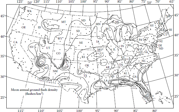
Any specific location within the country will either be on a contour or between counters. For example, Atlanta is between the 8 and 6 strikes/km2 counters but is very close to the 8 contour. Thus, a ground flash density of 8 should be used for Atlanta. Also, notice that the ground flash density for the whole State of California is two. This value can easily be converted into number of strikes/min2/year by multiplying it by 2.59. The resultant number of strikes should be rounded to the nearest whole number. For example, for Atlanta, 8 × 2.59 results in 21 strikes/min2/year, whereas for California, it is 5 strikes/min2/year. For an engineering design, the low end of the range of ground flash-density values can be taken as 50% of average. The high end of the range can be taken as 200% of average.
As Ben Franklin discovered it, lightning is attracted to tall structures, and this attraction is defined as an area shielded by the structure. This shielded area of the tower SA in m2 is determined from
where
N is the number of strikes to the tower
Ngfd is the average ground flash density in strikes/min2/year (found from Figure 10.41)
The number of strikes to a distribution or transmission line in open country (Noc) with a length of 100 km can be found from
where
b is the width between the outside conductors
h is the height of tower in m
or for a length of 1 km, it can be expressed as
For distribution lines, the width term b can be eliminated by assuming it zero. (It can be shown that the resultant error is less than 2.33%.) In addition by converting to English units, for a length of 1 mile,
For the total line length, where
where
s is the length of the lone in min
Ngfd is the average ground flash density in strikes/km2/year
For standard pole lengths (standard setting depths and REA standard construction), the total number of strikes to an open country distribution line can be expressed as
where C is a constant based on pole length.
For various standard pole lengths, the constant C is given in Table 10.14.
Constant C for REA Standard Pole Lengths
Pole Length, ft |
Setting Depth in soil, ft |
Conductor above the Pole Top, ft |
Height (h) of Line Aboveground, ft |
C = 0.022h0.6 |
|---|---|---|---|---|
30 |
5.5 |
0.66 |
25.16 |
0.154 |
35 |
6.0 |
0.66 |
29.16 |
0.168 |
40 |
6.0 |
0.66 |
34.66 |
0.185 |
45 |
6.5 |
0.66 |
39.16 |
0.199 |
50 |
7.0 |
0.66 |
43.66 |
0.212 |
Source: From Rural Electrification Administration: Guide for Making a Sectionalizing Study on Rural Electric Systems, REA Bulletin 61–2. March, 1958.
The total number of strikes to a distribution line is affected by the nearby trees, other structures, or objects that shield the line from direct strikes. Here, the shielding factor Sf can be defined as
where
N is the number of strikes to the shielded line
is the number of strikes to the line in open country
The methods used to determine the shielding factor are quite complex and involve the use of electrogeometric models. However, estimates of shielding effects can be made by considering standard shielding cases, and the accuracy of such estimates is sufficient for most engineering decisions.
Here, the value of Sf varies between 0.0 and 1.0:
If there is no shielding of any kind, then Sf = 0.
If there are tall trees on both sides of the line and within 100 ft of the line, then Sf = 0.90.
If there are tall trees at the edge of the typical 30 ft right of way (15 ft from the center of the line, on both sides), then Sf = 1.0.
If the trees present have heights that are 1.5 times the height of the line, then Sf = 0.70.
If the height of the one-sided shielding is twice the height of the line and within 50 ft of the line, Sf = 0.90.
If the shielding factor is known, the number of predicted direct strikes N to the lie is determined from
Example 10.7
Assume that the NL&NP Company of Kansas has 8000 customers on 2000 miles of line located in central Kansas that can be considered as an open country. The average pole length used on the distribution system is 35 ft. The distribution system has 6000 pole-mounted transformers installed. Determine the following:
- The average span length, if the system has 35,000 poles
- The number of strikes per mile per year
- The number of expected strikes to the adjoining spans of an equipment pole
- The total expected number of strikes to the adjoining spans of the 6000 transformer poles per year
- The average time between lightning strikes that can be expected within one span of an "average" equipment pole
Solution
- For the 35,000 poles, the average span length is
- From Figure 10.41, the ground flash density in central Kansas is 9 strikes/km2/year. For a 35 ft pole, from Table 10.14, C = 0.168. Therefore, the number of strikes is
- Since a direct lightning strike can be expected to cause a flashover on the first pole on either side of the strike point, only concern with the two spans on each side of the equipment location. Therefore, the number of expected strikes is
- The total expected number of strikes to the adjoining spans of the 6000 transformer poles per year is
- The average time between lightning strikes that can be expected within one span of an average equipment pole is
Example 10.8
Consider the distribution system used in Example 10.7 and assume that most transformers are shielded from lightning to some extent by buildings or trees. Therefore, use a "reasonable estimate" of 70% for the average shielding factor. It is assumed that 5% of lightning return sto exceed 100 kA. Determine the following:
- The total number of strikes per year to transformers if shielding is taken into consideration
- The total number of expected transformer failures per year due to lightning
- The annual expected transformer failure rate due to lightning
Solution
- If the shielding is used, then
- Since 5% of stoke currents exceed 100 kA, the expected number of transformer failures is
- The annual expected transformer failure rate due to lightning is
that is, 1 out of every 400 installed transformers.
Example 10.9
Consider the distribution system used in Example 10.7 and assume that for the arrester used on the system, a lightning current of 50 kA produces a discharge voltage of 95 kV. The arrester is tank mounted with zero lead length. The NL&NP Company uses 95 kV BIL transformers so that surge voltages in excess of 95 kV can be expected to cause transformer failure. For midspan lightning strikes, the lightning current will divide, and half of the current will flow down the line in each direction. Determine the following:
- The amount of lightning return stroke current if the transformer is to be subjected to a 50 kA current surge
- The total annual number of strikes to transformers that can be expected to produce voltages that exceed the transformer BIL and cause failures
Solution
- For the transformer to be subjected to a 50 kA current surge, it is required that the lightning return stroke current must be
- Since 5% of lightning return strokes exceed 100 kA,
Example 10.10
Assume that the NL&NP Company of California utilizes 30 ft poles in its 100 mile long rural lines. The practical maximum line width occurs with the use of an 8 ft crossarm and a horizontal conductor arrangement. The distance between the outside conductors is 7.4 ft. Assume that the 100 min long line is in open country. Determine the following:
- The number of strikes to the line
- The number of strikes to the line, if the line width term b is ignored and/or assumed to be zero
- Compare the results of parts, and express the difference in percentage Solution
Solution
- The number of strikes to the 100 min long line can be found from
where
Ngfd = 2 strikes/km2/year (from Figure 10.41)
b = (7.4 ft)(0.3048 m/ft) = 2.256 m
h = (25.16 ft)(0.3048 m/ft) = 7.669 m (25.16 ft is found from Table 10.14)
Thus,
- If the line width term b is ignored,
- Therefore
This 2.32% difference is a maximum value, and for taller or narrower lines, the difference is less than 2.32%.
10.16 Insulators
An insulator is a material that prevents the flow of an electric current and can be used to support electric conductors. The function of an insulator is to provide for the necessary clearances between the line conductors, between conductors and ground, and between conductors and the pole or tower. Insulators are made up of porcelain, glass, and fiberglass treated with epoxy resins. However, porcelain is still the most common material used for insulators.
The basic types of insulators include (1) pin-type insulators, (2) suspension insulators, and (3) strain insulators. The pin insulator gets its name from the fact that it is supported on a pin. The pin holds the insulator, and the insulator has the conductor tied to it. They may be made in one piece for voltages below 23 kV, in two pieces for voltages from 23 to 46 kV, in three pieces for voltages from 46 to 69 kV, and in four pieces for voltages from 69 to 88 kV. Pin insulators are used in distribution lines and are seldom used on transmission lines having voltages above 44 kV, although some 88 kV lines using pin insulators are in operation. The glass pin insulator is mainly used on low-voltage circuits. The porcelain pin insulator is used on secondary mains and services, as well as on primary mains, feeders, and transmission lines.
A modified version of the pin-type insulator is known as the post-type insulator. The post-type insulators are used on distribution, subtransmission, and transmission lines and are installed on wood, concrete, and steel poles. The line post insulators are usually made as one-piece solid porcelain units.
Suspension insulators are normally used on subtransmission and transmission lines and consist of a string of interlinking separate disks made of porcelain. A string may consist of many disks depending on the line voltage. (For further information, see Gönen [16, Chapter 4]). For example, as an average, 7 disks are usually used for 115 kV lines and 18 disks are usually used for 345 kV lines.
The suspension insulator, as its name implies, is suspended from the crossarm (or a pole or tower) and has the line conductor fastened to the lower end. When there is a dead end of the line or there is corner or a sharp curve, or the line crosses a river, etc., the line will withstand great strain.
The assembly of suspension units arranged to dead-end the conductor of such structure is called a dead-end, or strain, insulator. In such an arrangement, suspension insulators are used as strain insulators [16,17].
Problems
- 10.1 Repeat Example 10.1, assuming that the fault current is 1000 A.
- 10.2 Repeat Example 10.1, assuming that the fault current is 500 A.
- 10.3 In Problem 10.2, determine the lacking relay travel that is necessary for the relay to close its contacts and trip its breaker:
- (a) In percent
- (b) In seconds
- 10.4 Assume that an inverse-time-overcurrent relay is installed at a location on a feeder. It is desired that the substation OCB trip on a sustained current of approximately 400 A and trip in 2 s on a short-circuit current of 4000 A. Assuming that CTs of 60:1 ratio are used, determine the following:
- (a) The current-tap setting of the relay
- (b) The time setting of the relay
- 10.5 Repeat Example 10.2, assuming that the transformer is rated 3750 kVA 69/4.16 kV feeding a three-phase four-wire 4.16 kV circuit and that the sizes of the phase conductors and neutral conductor are 267AS33 and OAS7, respectively.
- 10.6 Repeat Example 10.3, assuming that the faults are bolted and that the fault impedance is 40 Ω.
- 10.7 Assume that there is a bolted fault at a certain point F on a distribution circuit, as indicated in Figure P10.1. Also assume that the maximum power generation of the system is 600 MVA. Determine the following:
- (a) Maximum values of the available three-phase, L–L, and SLG fault currents at the fault point F, using actual system values
- (b) Minimum value of the available SLG fault, assuming that it is equal to 60 percent of its maximum value found in part a
- 10.8 Repeat Example 10.4, assuming that the substation transformer’s impedance is 7.5 percent and that the distribution transformer has a capacity of 75 kVA with 2 percent impedance. Also assume that the primary line is made of three 477AS33 conductors and a neutral conductor of OAS7 at 62 in spacing and that the lengths of the primary line and secondary cable are 1000 and 50 ft, respectively. Assume that the impedance of the three-wire OALSSC secondary cable is 0.1843 + j0.0273 Ω/1000 ft.
- 10.9 Assume that the NL&NP Company of California has 6000 customers on 1000 miles of lines located in central California (which can be considered as an open country). The average pole length used on the distribution system has 4000 pole-mounted transformers installed. Determine the following:
- (a) The average span length, if the system has 17,032 poles
- (b) The number of strikes per mile per year
- (c) The number of expected strikes to the adjoining spans of an equipment pole
- (d) The total expected number of strikes to the adjoining spans of the 4000 transformer poles per year
- (e) The average time between lightning strikes that can be expected within one span of an “average” equipment pole
- 10.10 Consider the distribution system given in Problem 10.9 and assume that most transformers are shielded from lightning to some extent by buildings or trees. Therefore, use a “reasonable estimate” of 70% for the average shielding factor. It is assumed that the total expected number of strikes to the transformer poles is 174 strikes/year and that 5% of lightning return strokes exceed 100 kA. Determine the following:
- (a) The total number of strikes per year to the transformers if shielding is taken into consideration
- (b) The total number of expected transformer failures per year due to lightning
- (c) The annual expected transformer failure rate due to lightning
- 10.11 Consider the distribution system given in Problem 10.10, and assume that for the arrester used on the system, a lightning current of 50 kA produces a discharge voltage of 95 kV. The arrester is tank mounted with zero lead length. The NL&NP Company uses 95 kV BIL transformers so that surge voltages in excess of 95 kV can be expected to cause transformer failure. For midspan lightning strikes, the lightning current will divide, and half of the current will flow down the line in each direction. It is assumed that 5% of lightning return strokes exceed 100 kA. Determine the following:
- (a) The amount of lightning return stroke current if the transformer is to be subjected to a 50 kA current surge
- (b) The total annual number of strikes to transformers that can be expected to produce voltages that exceed the transformer BIL and cause failures
- 10.12 Resolve Example 10.3 by using MATLAB®.
- 10.13 Resolve Example 10.4 by using MATLAB.
References
1. Westinghouse Electric Corporation: Electric Utility Engineering Reference Book-Distribution Systems, vol. 3, Westinghouse Electric Corporation, East Pittsburgh, PA, 1965.
2. Fink, D. G. and H. W. Beaty: Standard Handbook for Electrical Engineers, 11th edn., McGraw-Hill, New York, 1978.
3. Anderson, P. M.: Elements of Power System Protection, Cyclone Copy Center, Ames, IA, 1975.
4. General Electric Company: Overcurrent Protection for Distribution Systems, Application Manual GET-1751A, Schenectady, NY, 1962.
5. General Electric Company: Distribution System Feeder Overcurrent Protection, Application Manual GET-6450, 1979.
6. Westinghouse Electric Corporation: Westinghouse Transmission and Distribution Reference Book, Westinghouse Electric Corporation, East Pittsburgh, PA, 1964.
7. IEEE: Recommended Practice for Protection and Coordination of Industrial and Commercial Power Systems, IEEE Standard 242-1975, New York, 1975.
8. Anderson, P. M.: Analysis of Faulted Power Systems, Iowa State University Press, Ames, IA, 1973.
9. Rural Electrification Administration: Guide for Making a Sectionalizing Study on Rural Electric Systems, REA Bulletin 61-2, March, 1958, US Dept. of Agriculture, Washington DC.
10. Wagner, C. F. and R. D. Evans: Symmetrical Components, McGraw-Hill, New York, 1933.
11. Stevenson, W. D.: Elements of Power System Analysis, 3rd edn., McGraw-Hill, New York, 1975.
12. Gross, C. A.: Power System Analysis, Wiley, New York, 1979.
13. Carson, J. R.: Wave propagation in overhead wires with ground return, Bell Syst. Tech. J., 5, October 1926, 539–555.
14. Aucoin, B. M. and B. D. Russell: Distribution high-impedance fault detection utilizing high-frequency current components, IEEE Trans. Power Appar. Syst., PAS-101(6), June 1982, 1596–1606.
15. IEEE: Detection of Downed Conductors on Utility Distribution Systems, IEEE Tutorial Course, prod. No. 90EHO310-3-PWR, 1989.
16. Gönen, T.: Modern Power System Analysis, Wiley, New York, 1988.
17. Gönen, T.: Electric Power Transmission System Engineering, Wiley, New York, 1988.
18. MacGorman, D. R. et al.: Lightning Strike Density for the Contiguous United States from Thunderstorm Duration Records, NUREG/CR-3759, National Oceanic and Atmospheric Administration, Prepared for the U. S. Nuclear Regulatory Commission, May 1984.
* TCC curves of overcurrent protective devices are plotted on log-log coordinate paper. The use of this standard-size transparent paper allows the comparison of curves by superimposing one sheet over another.
* For further information, see Ref. [5].
* More rigorous and detailed treatment of the subject is given by Anderson [3,8].
† One should keep in mind that these probabilities may differ substantially from one system to another in practice.
* Anderson [3] recommends letting the positive-sequence. Thevenin impedance of the system, that is, Zlsys be equal to zero, if there is no exact system information available and, at the same time, the substation transformer is small. Of course, by using this assumption, the system is treated as an infinitely large system.
* Remember that an impedance can be converted from one base voltage to another by using Z2 = Z1(V2/V1)2, where Z1 = impedance on V1 base and Z2 = impedance on V2 base.
† Note that there has been a shift in notation and the symbol Z1,T stands for Z1,T stands for ZT.
* Usually the resistance and reactance values of a substation transformer are approximately equal to 2% and 98% of its impedance, respectively.
* Note that there has been a shift in notation and the symbol ZT stands for Z1,T.
† Note that there has been a shift in notation and the symbol n stands for primary-to-secondary impedance-transfer ratio. (It is the inverse of the transformer turns ratio.)