Chapter 3
Application of Distribution Transformers
Now that I’m almost up the ladder,
I should, no doubt, be feeling gladder,
It is quite fine, the view and such,
If just it didn’t shake so much.Richard Armour
3.1 Introduction
In general, distribution transformers are used to reduce primary system voltages (2.4–34.5 kV) to utilization voltages (120–600 V). Table 3.1 gives standard transformer capacity and voltage ratings according to ANSI Standard C57.12.20-1964 for single-phase distribution transformers. Other voltages are also available, for example, 2400 × 7200, which is used on a 2400 V system that is to be changed later to 7200 V.
Standard Transformer Kilovoltamperes and Voltages
Kilovoltamperes |
High Voltages |
Low Voltages |
|||
|---|---|---|---|---|---|
Single Phase |
Three Phase |
Single Phase |
Three Phase |
Single Phase |
Three Phase |
5 |
30 |
2,400/4,160 Y |
2,400 |
120/240 |
208Y/120 |
10 |
45 |
4,800/8,320 Y |
4,160 Y/2,400 |
240/480 |
240 |
15 |
75 |
4,800Y/8,320 YX |
4,160 Y |
2400 |
480 |
25 |
112½ |
7,200/12,470 Y |
4,800 |
2520 |
480 Y/277 |
37½ |
150 |
12,470 Gnd Y/7,200 |
8,320 Y/4,800 |
4800 |
240 × 480 |
50 |
225 |
7,620/13,200 Y |
8,320 Y |
5040 |
2,400 |
75 |
300 |
13,200 Gnd Y/7,620 |
7,200 |
6900 |
4,160 Y/2,400 |
100 |
500 |
12,000 |
12,000 |
7200 |
4,800 |
167 |
13,200/22,860 Gnd Y |
12,470 Y/7,200 |
7560 |
12,470 Y/7,200 |
|
250 |
13,200 |
12,470 Y |
7980 |
13,200 Y/7,620 |
|
333 |
13,800 Gnd Y/7,970 |
13,200 Y/7,620 |
|||
500 |
13,800/23,900 Gnd Y |
13,200 Y |
|||
13,800 |
13,200 |
||||
14,400/24,940 Gnd Y |
13,800 |
||||
16,340 |
22,900 |
||||
19,920/34,500 Gnd Y |
34,400 |
||||
22,900 |
43,800 |
||||
34,400 |
67,000 |
||||
43,800 |
|||||
67,000 |
|||||
Secondary symbols used are the letter Y, which indicates that the winding is connected or may be connected in wye, and Gnd Y, which indicates that the winding has one end grounded to the tank or brought out through a reduced insulation bushing. Windings that are delta connected or may be connected delta are designated by the voltage of the winding only.
In Table 3.1, further information is given by the order in which the voltages are written for low-voltage (LV) windings. To designate a winding with a mid-tap that will provide half the fullwinding kilovoltampere rating at half the full-winding voltage, the full-winding voltage is written first, followed by a slant, and then the mid-tap voltage. For example, 240/120 is used for a three-wire connection to designate a 120 V mid-tap voltage with a 240 V full-winding voltage. A winding that is appropriate for series, multiple, and three-wire connections will have the designation of multiple voltage rating followed by a slant and the series voltage rating, for example, the notation 120/240 means that the winding is appropriate either for 120 V multiple connection, for 240 V series connection, and for 240/120 three-wire connection. When two voltages are separated by a cross (×), a winding that is appropriate for both multiple and series connections but not for three-wire connection is indicated. The notation 120 × 240 is used to differentiate a winding that can be used for 120 V multiple connection and 240 V series connection, but not a three-wire connection. Examples of all symbols used are given in Table 3.2.
Designation of Voltage Ratings for Single- and Three-Phase Distribution Transformers
Single Phase |
Three Phase |
||
|---|---|---|---|
Designation |
Meaning |
Designation |
Meaning |
120/240 |
Series, multiple, or three-wire connection |
2,400/4,160 Y |
Suitable for delta or wye connection |
240/120 |
Series or three-wire connection only |
4,160 Y |
Wye connection only (no neutral) |
240 × 480 |
Series or multiple connection only |
4,160 Y 2,400 |
Wye connection only (with neutral available) |
120/208 Y |
Suitable for delta or wye connection three phase |
12,470 Gnd Y/7,200 |
Wye connection only (with reduced insulation neutral available) |
12,470 Gnd Y/7,200 |
One end of winding grounded to tank or brought out through reduced insulation bushing |
4,160 |
Delta connection only |
To reduce installation costs to a minimum, small distribution transformers are made for pole mounting in overhead distribution. To reduce size and weight, preferred oriented steel is commonly used in their construction. Transformers 100 kVA and below are attached directly to the pole, and transformers larger than 100 up to 500 kVA are hung on crossbeams or support lugs. If three or more transformers larger than 100 kVA are used, they are installed on a platform supported by two poles.
In underground distribution, transformers are installed in street vaults, in manholes direct-buried, on pads at ground level, or within buildings. The type of transformer may depend upon soil content, lot location, public acceptance, or cost.
The distribution transformers and any secondary service junction devices are installed within elements, usually placed on either the front or the rear lot lines of the customer’s premises. The installation of the equipment to either front or rear locations may be limited by customer preference, local ordinances, landscape conditions, etc. The rule of thumb requires that a transformer be centrally located with respect to the load it supplies in order to provide proper cable economy, voltage drop, and aesthetic effect.
Secondary service junctions for an underground distribution system can be of the pedestal, hand-hole, or direct-buried splice types. No junction is required if the service cables are connected directly from the distribution transformer to the user’s apparatus.
Secondary or service conductors can be either copper or aluminum. However, in general, aluminum conductors are mostly used for cost savings. The cables are either single conductor or triplex conductors. Neutrals may be either bare or covered, installed separately, or assembled with the power conductors. All secondary or service conductors are rated 600 V, and their sizes differ from # 6 AWG to 1000 kcmil.
3.2 Types of Distribution Transformers
Heat is a limiting factor in transformer loading. Removing the coil heat is an important task. In liquid-filled types, the transformer coils are immersed in a smooth-surfaced, oil-filled tank. Oil absorbs the coil heat and transfers it to the tank surface, which, in turn, delivers it to the surrounding air. For transformers 25 kVA and larger, the size of the smooth tank surface required to dissipate heat becomes larger than that required to enclose the coils. Therefore, the transformer tank may be corrugated to add surface, or external tubes may be welded to the tank. To further increase the heat-disposal capacity, air may be blown over the tube surface. Such designs are known as forcedair-cooled, with respect to self-cooled types. Presently, however, all distribution transformers are built to be self-cooled.
Therefore, the distribution transformers can be classified as (1) dry type and (2) liquid-filled type. The dry-type distribution transformers are air-cooled and air-insulated. The liquid-filled-type distribution transformers can further be classified as (1) oil filled and (2) inerteen filled.
The distribution transformers employed in overhead distribution systems can be categorized as
- Conventional transformers
- Completely self-protecting (CSP) transformers
- Completely self-protecting for secondary banking (CSPB) transformers
The conventional transformers have no integral lightning, fault, or overload protective devices provided as a part of the transformer. The CSP transformers are, as the name implies, self-protecting from lightning or line surges, overloads, and short circuits. Lightning arresters mounted directly on the transformer tank, as shown in Figure 3.1, protect the primary winding against the lightning and line surges. The overload protection is provided by circuit breakers inside the transformer tank. The transformer is protected against an internal fault by internal protective links located between the primary winding and the primary bushing. Single-phase CSP transformers (oil-immersed, polemounted, 65°C, 60 Hz, 10–500 kVA) are available for a range of primary voltages from 2,400 to 34,400 V. The secondary voltages are 120/240 or 240/480/277 V. The CSPB distribution transformers are designed for banked secondary service. They are built similar to the CSP transformers, but they are provided with two sets of circuit breakers. The second set is used to sectionalize the secondary when it is needed.

Overhead pole-mounted distribution transformers: (a) single-phase completely self-protecting (or conventional) and (b) three phase.
(From Westinghouse Electric Corporation, East Pittsburgh, PA. With permission.)
The distribution transformers employed in underground distribution systems can be categorized as
- Subway transformers
- Low-cost residential transformers
- Network transformers
Subway transformers are used in underground vaults. They can be conventional type or current-protected type. Low-cost residential transformers are similar to those conventional transformers employed in overhead distribution. Network transformers are employed in secondary networks. They have the primary disconnecting and grounding switch and the network protector mounted integrally on the transformer. They can be either liquid filled, ventilated dry type, or sealed dry type.
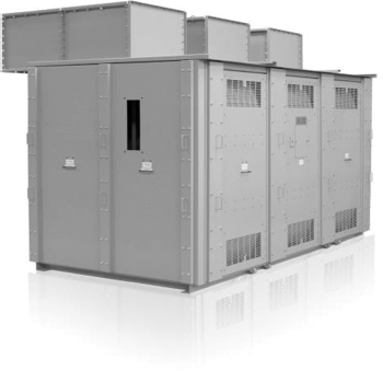
The ABB Corporation developed resibloc dry-type distribution transformers from 112.5 through 25,000 kVA, and from 2,300 through 34.5 kV primary voltage level and 120 V through 15 kV secondary voltage level. Such transformers have windings that are hermetically cast in epoxy without the use of mold. The epoxy insulation system is reinforced by a special glass fiber roving technique that binds the coil together into virtual winding block. As a result, they have unsurpassed mechanical strength with design optimization through 25,000 kVA. Figure 3.2 shows such resibloc network transformer. Figure 3.3 shows a dry-type pole-mounted resibloc transformer. Figure 3.4 shows a dry-type resibloc network transformer. Figure 3.5 shows an outdoor three-phase dry-type resibloc transformer. Figure 3.6 shows a pad-mount-type single-phase resibloc transformer. Figure 3.7 shows a pad-mount three-phase resibloc transformer. Figure 3.8 shows an arch flash-resistant drytype three-phase resibloc transformer. Figure 3.9 shows a TRIDRY dry-type resibloc transformer. Figure 3.10 shows a VPI dry resibloc transformer. Figure 3.11 shows a pad-mount installation of three-phase resibloc transformer.


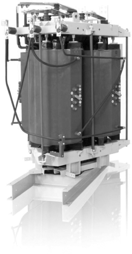
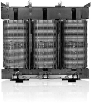
These resibloc transformers provide the ultimate withstand to thermal and mechanical stresses from severe climates, cycling loads, and short circuit forces. The epoxy insulation system is highly resistant to moisture, freezing, and chemicals, and is used in most demanding applications. Such transformers are nonexplosive with resistance to flame and do not require vaults, containment dikes, or expensive fire suppression systems. Primary basic impulse insulation level (BIL) is up to 150 kV and secondary BIL is up to 75 kV.
They can withstand a temperature rise of 80°C. They have no danger of fire and explosion and have no liquids to leak. Thus, they require minimal maintenance. They can be used indoor and outdoor enclosures. The resibloc transformers will not ignite during an electrical arc of nominal duration. If ignited with a direct flame, resibloc will self-extinguish when the flame is removed.
Resibloc transformers are utilized in some of the harshest indoor and outdoor environments imaginable. However, while core and coil technologies have been enhanced to combat caustic and humid environments, resibloc transformers still require the protection of a properly designed enclosure. An enclosure that flexes or bends under high wind loading can compromise electrical clearances from the transformer to the enclosure, which can lead to transformer failures as well as electrical safety hazards.
For example, an enclosure that allows excess water entry into it also poses unique risk. Such enclosure designs have been used along coastal areas and frigid northern slopes where high winds and driving rain are common. They can be also supplied with forced air cooling. The temperature sensors are located in the LV windings and are connected to the three-phase winding temperature monitor that controls the forced air cooling automatically.
Figure 3.12 shows various types of transformers. Figure 3.12a shows a typical secondary-unit substation with the high voltage (HV) and the LV on opposite ends and full-length flanges for close coupling to HV and LV switchgears. These units are normally made in sizes from 75 to 2500 kVA, three-phase, to 35 kV class. A typical single-phase pole-type transformer for a normal utility application is shown in Figure 3.12b. These are made from 10 to 500 kVA for delta and wye systems (one-bushing or two-bushing HV).
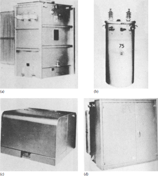
Various types of transformer: (a) a typical secondary unit substation transformer, (b) a typical single-phase pole-type tansformer, (c) a single-phase pad-mounted transformer, and (d) three-phase pad-mounted transformer.
(From Baleau Standard Inc., with permission.)
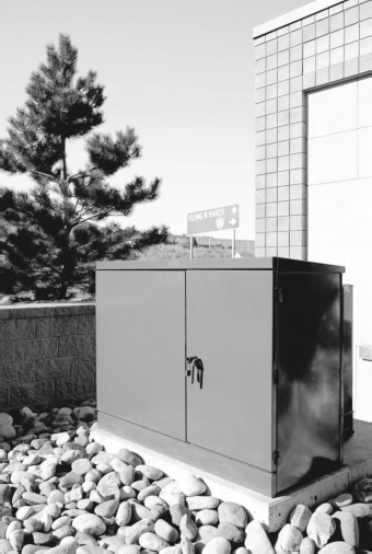
Figure 3.12c shows a typical single-phase pad-mounted (minipad) utility-type transformer. These are made from 10 to 167 kVA. They are designed to do the same function as the pole type except they are for the underground distribution system where all cables are below grade. A typical threephase pad-mounted (stan-pad) transformer used by utilities as well as industrial and commercial applications is shown in Figure 3.12d. They are made from 45 to 2500 kVA normally, but have been made to 5000 kVA on special applications. They are also designed for underground service.
Figure 3.13 shows various types of transformers. Figure 3.13a shows a typical three-phase subsurface-vault-type transformer used in utility applications in vaults below grade where there is no room to place the transformer elsewhere. These units are made for 75–2500 kVA and are made of a heavier-gage steel, special heavy corrugated radiators for cooling, and a special coal-tar type of paint.

Various types of transformers: (a) three-phase sub-surface-vault type transformer, (b) a typical mobile transformer, and (c) a typical power transformer.
(From Baleau Standard Inc., with permission.)
A typical mobile transformer is shown in Figure 3.13b. These units are made for emergency applications and to allow utilities to reduce inventory. They are made typically for 500–2500 kVA. They can be used on underground service as well as overhead service. Normally they can have two or three primary voltages and two or three secondary voltages, so they may be used on any system the utility may have. For an emergency outage, this unit is simply driven to the site, hooked up, and the power to the site is restored. This allows time to analyze and repair the failed unit. Figure 3.13c shows a typical power transformer. This class of unit is manufactured from 3700 kVA to 30 MVA up to about 138 kV class. The picture shows removable radiators to allow for a smaller size during shipment, and fans for increased capacity when required, including an automatic on-load tap changer that changes as the voltage varies.
Table 3.3 presents electrical characteristics of typical single-phase distribution transformers. Table 3.4 gives electrical characteristics of typical three-phase pad-mounted transformers. (For more accurate values, consult the individual manufacturer’s catalogs.)
Electrical Characteristics of Typical Single-Phase Distribution Transformersa
120/240 V Low |
240/480 and 277/480 YVM |
|||||||||||||||
|---|---|---|---|---|---|---|---|---|---|---|---|---|---|---|---|---|
Percent of A v. |
Watts Loss |
% |
% |
% |
Watts Loss |
% |
% |
% |
||||||||
kVA |
Excit. Curr. |
No Load |
Total |
1.0 PF |
0.8 PF |
Z |
R |
X |
No Load |
Total |
1.0 PF |
0.8 PF |
Z |
R |
X |
|
2400/4160 Y V high voltage |
||||||||||||||||
5 |
2.4 |
34 |
137 |
2.06 |
2.12 |
2.2 |
2.1 |
0.8 |
||||||||
10 |
1.6 |
68 |
197 |
1.30 |
1.68 |
1.7 |
1.3 |
1.1 |
68 |
202 |
1.35 |
1.69 |
1.7 |
1.3 |
1.0 |
|
15 |
1.4 |
84 |
272 |
1.27 |
1.59 |
1.6 |
1.3 |
1.0 |
84 |
277 |
1.30 |
1.60 |
1.6 |
1.3 |
1.1 |
|
25 |
1.3 |
118 |
385 |
1.10 |
1.65 |
1.7 |
1.1 |
1.1 |
118 |
390 |
1.11 |
1.65 |
1.7 |
1.1 |
1.3 |
|
38 |
1.1 |
166 |
540 |
1.00 |
1.55 |
1.6 |
1.0 |
1.3 |
166 |
550 |
1.04 |
1.54 |
1.6 |
1.0 |
1.2 |
|
50 |
1.0 |
185 |
615 |
0.88 |
1.58 |
1.7 |
0.9 |
1.5 |
185 |
625 |
0.90 |
1.58 |
1.7 |
0.9 |
1.5 |
|
75 |
1.3 |
285 |
910 |
0.85 |
1.41 |
1.5 |
0.8 |
1.2 |
285 |
925 |
0.86 |
1.33 |
1.4 |
0.9 |
1.1 |
|
100 |
1.2 |
355 |
1175 |
0.84 |
1.55 |
1.7 |
0.8 |
1.5 |
355 |
1190 |
0.85 |
1.49 |
1.6 |
0.8 |
1.4 |
|
167 |
1.0 |
500 |
2100 |
0.99 |
1.75 |
1.9 |
1.0 |
1.6 |
500 |
2000 |
0.90 |
1.57 |
1.7 |
0.9 |
1.4 |
|
250 |
1.0 |
610 |
3390 |
1.16 |
2.16 |
2.4 |
1.1 |
2.1 |
610 |
3280 |
1.11 |
2.02 |
2.2 |
1.1 |
1.9 |
|
333 |
1.0 |
840 |
4200 |
1.08 |
2.51 |
3.0 |
1.0 |
2.8 |
840 |
3690 |
0.88 |
1.90 |
2.2 |
0.9 |
1.9 |
|
500 |
1.0 |
1140 |
5740 |
0.97 |
2.50 |
3.1 |
0.9 |
3.0 |
1140 |
4810 |
0.95 |
2.00 |
2.3 |
0.7 |
2.2 |
|
7,200/12,470 Y V high voltage |
||||||||||||||||
5 |
2.4 |
41 |
144 |
2.07 |
2.11 |
2.2 |
2.1 |
0.8 |
||||||||
10 |
1.6 |
68 |
204 |
1.37 |
1.80 |
1.8 |
1.4 |
1.2 |
68 |
209 |
1.43 |
1.80 |
1.8 |
1.4 |
1.1 |
|
15 |
1.4 |
84 |
282 |
1.33 |
1.69 |
1.7 |
1.3 |
1.2 |
84 |
287 |
1.35 |
1.70 |
1.7 |
1.4 |
1.0 |
|
25 |
1.3 |
118 |
422 |
1.22 |
1.69 |
1.7 |
1.2 |
1.2 |
118 |
427 |
1.24 |
1.69 |
1.7 |
1.2 |
1.2 |
|
38 |
1.1 |
166 |
570 |
1.10 |
1.64 |
1.7 |
1.1 |
1.3 |
166 |
575 |
1.10 |
1.65 |
1.7 |
1.1 |
1.3 |
|
50 |
1.0 |
185 |
720 |
1.10 |
1.71 |
1.8 |
1.1 |
1.4 |
185 |
725 |
1.10 |
1.71 |
1.8 |
1.1 |
1.4 |
|
75 |
1.3 |
285 |
985 |
0.95 |
1.60 |
1.7 |
0.9 |
1.4 |
285 |
1000 |
0.97 |
1.52 |
1.6 |
1.0 |
1.3 |
|
100 |
1.2 |
355 |
1275 |
0.95 |
1.72 |
1.9 |
1.9 |
1.7 |
355 |
1290 |
0.95 |
1.60 |
1.7 |
1.9 |
1.4 |
|
167 |
1.0 |
500 |
2100 |
0.98 |
1.90 |
2.1 |
1.0 |
1.9 |
500 |
2000 |
0.91 |
1.70 |
1.9 |
0.9 |
1.7 |
|
250 |
1.0 |
610 |
3490 |
1.22 |
2.45 |
2.8 |
1.2 |
2.6 |
610 |
3250 |
1.17 |
2.19 |
2.4 |
1.1 |
2.2 |
|
333 |
1.0 |
840 |
4255 |
1.07 |
2.50 |
3.0 |
1.0 |
2.8 |
840 |
3690 |
0.89 |
2.03 |
2.4 |
0.9 |
2.2 |
|
500 |
1.0 |
1140 |
5640 |
0.95 |
2.55 |
3.2 |
0.9 |
3.1 |
1140 |
4810 |
0.78 |
1.99 |
2.4 |
0.7 |
2.3 |
|
13,200/22,860 Gnd Y or 13,800/23,900 Gnd Y or 14,400/24,940 Gnd Y V high voltage |
||||||||||||||||
5 |
2.4 |
42 |
154 |
2.25 |
2.30 |
2.4 |
2.3 |
0.9 |
||||||||
10 |
1.6 |
73 |
215 |
1.45 |
1.89 |
1.9 |
1.4 |
1.3 |
73 |
220 |
1.49 |
1.89 |
1.9 |
1.5 |
1.2 |
|
15 |
1.4 |
84 |
305 |
1.48 |
1.80 |
1.8 |
1.5 |
1.0 |
84 |
310 |
1.52 |
1.80 |
1.8 |
1.5 |
1.0 |
|
25 |
1.3 |
118 |
437 |
1.29 |
1.79 |
1.8 |
1.3 |
1.3 |
118 |
442 |
1.30 |
1.78 |
1.8 |
1.3 |
1.2 |
|
38 |
1.1 |
166 |
585 |
1.15 |
1.72 |
1.8 |
1.1 |
1.4 |
166 |
590 |
1.16 |
1.72 |
1.8 |
1.1 |
1.4 |
|
50 |
1.0 |
185 |
735 |
1.14 |
1.81 |
1.9 |
1.1 |
1.4 |
185 |
740 |
1.15 |
1.81 |
1.9 |
1.1 |
1.5 |
|
75 |
1.4 |
285 |
1050 |
1.05 |
1.78 |
1.8 |
1.0 |
1.5 |
285 |
1065 |
1.06 |
1.78 |
1.8 |
1.0 |
1.5 |
|
100 |
1.3 |
355 |
1300 |
0.97 |
1.81 |
2.0 |
0.9 |
1.8 |
355 |
1310 |
0.98 |
1.74 |
1.9 |
1.0 |
1.6 |
|
167 |
1.0 |
500 |
2160 |
0.98 |
1.96 |
2.2 |
1.0 |
2.0 |
500 |
2060 |
0.95 |
1.80 |
2.0 |
0.9 |
1.8 |
|
250 |
1.0 |
610 |
3490 |
1.22 |
2.52 |
2.9 |
1.2 |
2.7 |
610 |
3285 |
1.11 |
2.16 |
2.5 |
1.1 |
2.3 |
|
333 |
1.0 |
840 |
4300 |
1.09 |
2.60 |
3.1 |
1.0 |
2.9 |
840 |
3750 |
0.91 |
2.05 |
2.4 |
0.9 |
2.2 |
|
500 |
1.0 |
1140 |
5640 |
0.95 |
2.55 |
3.2 |
1.1 |
3.0 |
1140 |
4760 |
0.76 |
1.98 |
2.4 |
0.7 |
2.3 |
|
Electrical Characteristics of Typical Three-Phase Pad-Mounted Transformers
208 Y /120 V Low Voltage% Regulation |
480 Y /277 V Low Voltage% Regulation |
|||||||||||||||
|---|---|---|---|---|---|---|---|---|---|---|---|---|---|---|---|---|
Percent of A v. |
Watts Loss |
% |
% |
% |
Watts Loss |
% |
% |
% |
||||||||
kVA |
Excit. Curr. |
No Load |
Total |
1.0 PF |
0.8 PF |
Z |
R |
X |
No Load |
Total |
1.0 PF |
0.8 PF |
Z |
R |
X |
|
4,160 Gnd Y/2,400 X 12,470 Gnd Y/7,200 V high voltage |
||||||||||||||||
75 |
1.5 |
360 |
1,350 |
1.35 |
2.1 |
2.1 |
1.3 |
1.6 |
360 |
1,350 |
1.35 |
2.1 |
2.1 |
1.3 |
1.6 |
|
112 |
1.0 |
530 |
1,800 |
1.15 |
1.7 |
1.7 |
1.1 |
1.3 |
530 |
1,800 |
1.15 |
1.7 |
1.7 |
1.1 |
1.3 |
|
150 |
1.0 |
560 |
2,250 |
1.15 |
1.9 |
1.9 |
1.1 |
1.6 |
560 |
2,250 |
1.15 |
1.9 |
1.9 |
1.1 |
1.6 |
|
225 |
1.0 |
880 |
3,300 |
1.10 |
1.9 |
1.9 |
1.1 |
1.6 |
800 |
3,300 |
1.10 |
1.9 |
1.9 |
1.1 |
1.6 |
|
300 |
1.0 |
1050 |
4,300 |
1.10 |
1.9 |
2.0 |
1.1 |
1.7 |
1050 |
4,100 |
1.05 |
1.8 |
1.8 |
1.0 |
1.5 |
|
500 |
1.0 |
1600 |
6,800 |
1.15 |
2.2 |
2.3 |
1.0 |
2.1 |
1600 |
6,500 |
1.10 |
2.0 |
2.0 |
1.0 |
1.7 |
|
750 |
1.0 |
1800 |
10,200 |
1.28 |
4.4 |
5.7 |
1.1 |
5.6 |
1800 |
9,400 |
1.18 |
4.3 |
5.7 |
1.0 |
5.6 |
|
1000 |
1.0 |
2100 |
12,500 |
1.20 |
4.3 |
5.7 |
1.0 |
5.6 |
2100 |
10,900 |
1.04 |
4.2 |
5.7 |
0.9 |
5.7 |
|
1500 |
1.0 |
2900 |
19,400 |
1.26 |
4.3 |
5.7 |
1.1 |
5.6 |
3300 |
16,500 |
1.04 |
4.2 |
5.7 |
0.9 |
5.7 |
|
2500 |
1.0 |
4800 |
26,600 |
1.03 |
4.2 |
5.7 |
0.9 |
5.7 |
||||||||
3750 |
1.0 |
6500 |
35,500 |
0.95 |
4.1 |
5.7 |
0.8 |
5.7 |
||||||||
12,470 Grid Y/7,200 V high voltage |
||||||||||||||||
75 |
1.5 |
360 |
1,350 |
1.4 |
1.7 |
1.7 |
1.3 |
1.1 |
360 |
1,350 |
1.4 |
1.5 |
1.5 |
1.3 |
0.8 |
|
112 |
1.0 |
530 |
1,800 |
1.2 |
1.5 |
1.5 |
1.1 |
1.0 |
530 |
1,800 |
1.2 |
1.3 |
1.3 |
1.1 |
0.7 |
|
150 |
1.0 |
560 |
2,250 |
1.2 |
1.8 |
1.9 |
1.1 |
1.6 |
560 |
2,250 |
1.2 |
1.7 |
1.7 |
1.1 |
1.3 |
|
225 |
1.0 |
880 |
3,300 |
1.1 |
1.8 |
1.8 |
1.1 |
1.4 |
880 |
3,300 |
1.1 |
1.6 |
1.6 |
1.1 |
1.2 |
|
300 |
1.0 |
1050 |
4,300 |
1.1 |
1.6 |
1.6 |
1.1 |
1.2 |
1050 |
4,100 |
1.1 |
1.4 |
1.4 |
1.0 |
1.0 |
|
500 |
1.0 |
1600 |
6,800 |
1.1 |
1.7 |
1.7 |
1.0 |
1.4 |
1600 |
6,500 |
1.1 |
1.4 |
1.4 |
1.0 |
1.0 |
|
750 |
1.0 |
1800 |
10,200 |
1.3 |
4.4 |
5.7 |
1.1 |
5.6 |
1800 |
9,400 |
1.2 |
4.3 |
5.7 |
1.0 |
5.6 |
|
1000 |
1.0 |
2100 |
12,500 |
1.2 |
4.3 |
5.7 |
1.0 |
5.6 |
2100 |
10,900 |
1.0 |
4.2 |
5.7 |
0.9 |
5.7 |
|
1500 |
1.0 |
2900 |
19,400 |
1.3 |
4.3 |
5.7 |
1.1 |
5.6 |
3300 |
16,500 |
1.0 |
4.2 |
5.7 |
0.9 |
5.7 |
|
2500 |
1.0 |
4800 |
26,600 |
1.0 |
4.2 |
5.7 |
0.9 |
5.7 |
||||||||
3750 |
1.0 |
6500 |
35,500 |
0.9 |
4.1 |
5.7 |
0.8 |
5.7 |
||||||||
2400/4160 Y/2400 V low voltage |
||||||||||||||||
12,470 Delta V high voltage |
||||||||||||||||
1000 |
1.38 |
2443 |
11,480 |
1.06 |
4.09 |
5.56 |
0.89 |
5.49 |
||||||||
1500 |
1.33 |
3455 |
15,716 |
0.98 |
4.04 |
5.56 |
0.81 |
5.51 |
||||||||
2500 |
1.29 |
4956 |
23,193 |
0.92 |
3.97 |
5.56 |
0.73 |
5.52 |
||||||||
3750 |
1.37 |
6775 |
33,100 |
0.89 |
3.97 |
5.50 |
0.70 |
5.45 |
||||||||
5000 |
1.33 |
8800 |
42,125 |
0.86 |
3.94 |
5.50 |
0.67 |
5.45 |
||||||||
24,940 Delta V high voltage |
||||||||||||||||
1000 |
1.42 |
2533 |
11,588 |
1.07 |
4.09 |
5.56 |
0.91 |
5.49 |
||||||||
1500 |
1.37 |
3625 |
15,213 |
0.96 |
4.03 |
5.56 |
0.80 |
5.50 |
||||||||
2500 |
1.31 |
5338 |
23,213 |
0.88 |
3.98 |
5.56 |
0.72 |
5.52 |
||||||||
3750 |
1.42 |
7075 |
33,700 |
0.90 |
3.97 |
5.50 |
0.71 |
5.44 |
||||||||
5000 |
1.33 |
8725 |
43,550 |
0.88 |
3.96 |
5.50 |
0.69 |
5.44 |
||||||||
To find the resistance (R') and the reactance (X') of a transformer of equal size and voltage, which has a different impedance value (Z') than the one shown in tables, multiply the tabulated percent values of R and X by the ratio of the new impedance value to the tabulated impedance value, that is, Z'/Z. Therefore, the resistance and the reactance of the new transformer can be found from
R'=R×Z'Z %Ω(3.1)
and
X'=X×Z'Z %Ω(3.2)
3.3 Regulation
To calculate the transformer regulation for a kilovoltampere load of power factor cos θ, at rated voltage, any one of the following formulas can be used:
%regulation=SLST[%IRcosθ+%IXsinθ+(%IXcosθ−%IRsinθ)2200](3.3)
or
%regulation=IopIra[%Rcosθ+%Xsinθ+(%Xcosθ−%Rsinθ)2200](3.4)
or
%regulation=VRcosθ+VXsinθ+(VXcosθ−VRsinθ)2200(3.5)
where
θ is the power factor angle of load
VR is the percent resistance voltage
=copper lossoutput×100
SL is the apparent load power
ST is the rated apparent power of transformer
Iop is the operating current
Ira is the rated current
VX is the percent leakage reactance voltage
=(V2Z−V2R)1/2
VZ is the percent impedance voltage
Note that the percent regulation at unity power factor is
%Regulation=Copper lossOutput×100+(%reactance)2200(3.6)
3.4 Transformer Efficiency
The efficiency of a transformer can be calculated from
%Efficiency=Output in wattsOutput in watts + Total losses in watts×100(3.7)
The total losses include the losses in the electric circuit, magnetic circuit, and dielectric circuit. Stigant and Franklin [3, p. 97] state that a transformer has its highest efficiency at a load at which the iron loss and copper loss are equal. Therefore, the load at which the efficiency is the highest can be found from
%Load=(Iron lossCopper loss)1/2×100(3.8)
Figures 3.14 and 3.15 show nomograms for quick determination of the efficiency of a transformer. (For more accurate values, consult the individual manufacturer’s catalogs.) With the cost of electric energy presently 5–6 cents/kWh and projected to double within the next 10–15 years, as shown in Figure 3.16, the cost efficiency of transformers now shifts to align itself with energy efficiency.
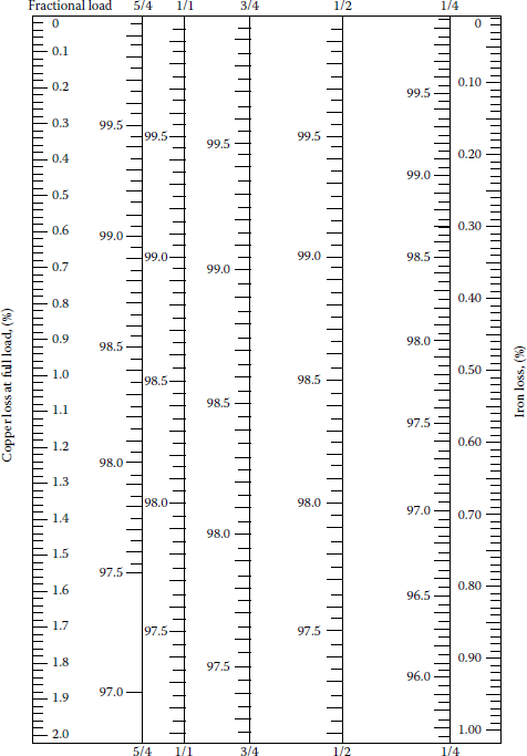
Transformer efficiency chart applicable only to the unity PF condition. To obtain the efficiency at a given load, lay a straightedge across the iron and copper loss values and read the efficiency at the point where the straightedge cuts the required load ordinate.
(From Stigant, S.A. and Franklin, A.C., The J&P Transformer Book, Butterworth, London, U.K., 1973.)
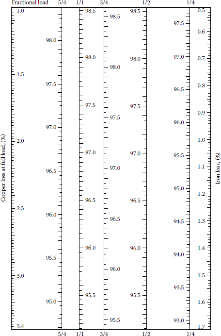
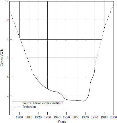
Cost of electric energy.
(From Stigant, S.A. and Franklin, A.C., The J&P Transformer Book, Butterworth, London, U.K., 1973. With permission.)
Note that the iron losses (or core losses) include (1) hysteresis loss and (2) eddy-current loss. The hysteresis loss is due to the power requirement of maintaining the continuous reversals of the elementary magnets (or individual molecules) of which the iron is composed as a result of the flux alternations in a transformer core. The eddy-current loss is the loss due to circulating currents in the core iron, caused by the magnetic flux in the iron cutting the iron, which is a conductor. The eddycurrent loss is proportional to the square of the frequency and the square of the flux density. The core is built up of thin laminations insulated from each other by an insulating coating on the iron to reduce the eddy-current loss. Also, in order to reduce the hysteresis loss and the eddy-current loss, special grades of steel alloyed with silicon are used. The iron or core losses are practically independent of the load. On the other hand, the copper losses are due to the resistance of the primary and secondary windings.
In general, the distribution transformer costs can be classified as (1) the cost of investment, (2) the cost of lost energy due to the losses in the transformer, and (3) the cost of demand lost (i.e., the cost of lost capacity) due to the losses in the transformer. Of course, the cost of investment is the largest cost component, and it includes the cost of the transformer itself and the costs of material and labor involved in the transformer installation.
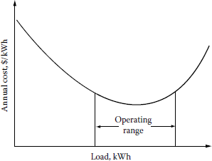
Figure 3.17 shows the annual cost per unit load vs. load level. At low-load levels, the relatively high costs result basically from the investment cost, whereas at high-load levels, they are due to the cost of additional loss of life of the transformer, the cost of lost energy, and the cost of demand loss in addition to the investment cost. Figure 3.15 indicates an operating range close to the bottom of the curve. Usually, it is economical to install a transformer at approximately 80% of its nameplate rating and to replace it later, at approximately 180%, by one with a larger capacity. However, presently, increasing costs of capital, plant and equipment, and energy tend to reduce these percentages.
3.5 Terminal or Lead Markings
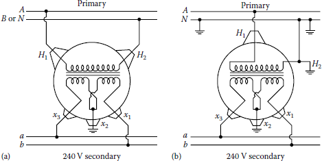
The terminals or leads of a transformer are the points to which external electric circuits are connected. According to NEMA and ASA standards, the higher-voltage winding is identified by HV or H, and the lower-voltage winding is identified by LV or x. Transformers with more than two windings have the windings identified as H, x, y, and z, in the order of decreasing voltage. The terminal H1 is located on the right-hand side when facing the HV side of the transformer. On single-phase transformers, the leads are numbered so that when H1 is connected to x1, the voltage between the highest-numbered H lead and the highest-numbered x lead is less than the voltage of the HV winding.
On three-phase transformers, the terminal H1 is on the right-hand side when facing the HV winding, with the H2 and H3 terminals in numerical sequence from right to left. The terminal x1 is on the left-hand side when facing the LV winding, with the x2 and x3 terminals in numerical sequence from left to right.
3.6 Transformer Polarity
Transformer-winding terminals are marked to show polarity, to indicate the HV from the LV side. Primary and secondary are not identified as such because which is which depends on input and output connections.
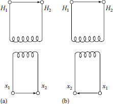
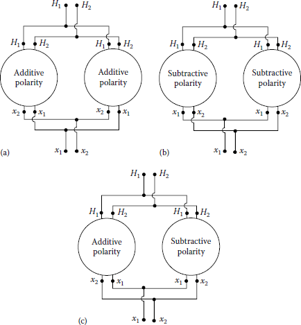
Transformer polarity is an indication of the direction of current flowing through the HV leads with respect to the direction of current flow through the LV leads at any given instant. In other words, the transformer polarity simply refers to the relative direction of induced voltages between the HV leads and the LV terminals. The polarity of a single-phase distribution transformer may be additive or subtractive. With standard markings, the voltage from H1 to H2 is always in the same direction or in phase with the voltage from X1 to X2. In a transformer where H1 and X1 terminals are adjacent, as shown in Figure 3.18a, the transformer is said to have subtractive polarity. On the other hand, when terminals H1 and X1 are diagonally opposite, as shown in Figure 3.18b, the transformer is said to have additive polarity.
Additive and subtractive polarity connections: (a) subtractive polarity and (b) additive polarity.
Transformer polarity can be determined by performing a simple test in which two adjacent terminals of the HV and LV windings are connected together and a moderate voltage is applied to the HV winding, as shown in Figure 3.19, and then the voltage between the HV and LV winding terminals that are not connected together are measured. The polarity is subtractive if the voltage read is less than the voltage applied to the HV winding, as shown in Figure 3.19a. The polarity is additive if the voltage read is greater than the applied voltage, as shown in Figure 3.19b.

By industry standards, all single-phase distribution transformers 200 kVA and smaller, having HVs 8660 V and below (winding voltages), have additive polarity. All other single-phase transformers have a subtractive polarity. Polarity markings are very useful when connecting transformers into three-phase banks.
3.7 Distribution Transformer Loading Guides
The rated kilovoltamperes of a given transformer is the output that can be obtained continuously at rated voltage and frequency without exceeding the specified temperature rise. Temperature rise is used for rating purposes rather than actual temperature, since the ambient temperature may vary considerably under operating conditions. The life of insulation commonly used in transformers depends upon the temperature the insulation reaches and the length of time that this temperature is sustained. Therefore, before the overload capabilities of the transformer can be determined, the ambient temperature, preload conditions, and the duration of peak loads must be known.
Based on Appendix C57.91 entitled The Guide for Loading Mineral Oil-Immersed Overhead-Type Distribution Transformers with 55°C and 65°C Average Winding Rise [4], which is an appendix to the ANSI Overhead Distribution Standard C57.12, 20 transformer insulation-life curves were developed. These curves indicate a minimum life expectancy of 20 years at 95°C and 110°C hotspot temperatures for 55°C and 65°C rise transformers. Previous transformer loading guides were based on the so-called 8°C insulation-life rule. For example, for transformers with class A insulation (usually oil filled), the rate of deterioration doubles approximately with each 8°C increase in temperature. In other words, if a class A insulation transformer were operated 8°C above its rated temperature, its life would be cut in half.
3.8 Equivalent Circuits of a Transformer
It is possible to use several equivalent circuits to represent a given transformer. However, the general practice is to choose the simplest one, which would provide the desired accuracy in calculations.
Figure 3.20 shows an equivalent circuit of a single-phase two-winding transformer. It represents a practical transformer with an iron core and connected to a load (ZL). When the primary winding is excited, a flux is produced through the iron core. The flux that links both primary and secondary is called the mutual flux, and its maximum value is denoted as ϕm. However, there are also leakage fluxes ϕl1 and ϕl2 that are produced at the primary and secondary windings, respectively. In turn, the ϕl1 and ϕl2 leakage fluxes produce xl1 and xl2, that is, primary and secondary inductive reactances, respectively. The primary and secondary windings also have their internal resistances of r1 and r2.
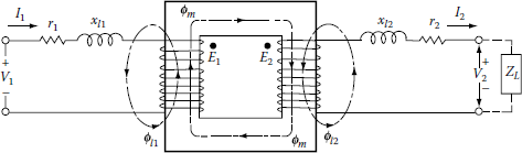
Figure 3.21 shows an equivalent circuit of a loaded transformer. Note that I'2 current is a primarycurrent (or load) component that exactly corresponds to the secondary current I2, as it does for an ideal transformer. Therefore,
I'2=n2n1×I2(3.9)
or
I'2=I2n(3.10)
where
I2 is the secondary current
n1 is the number of turns in primary winding
n2 is the number of turns in secondary winding
n is the turns ratio =n1n2
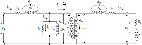
The Ie current is the excitation current component of the primary current I1 that is needed to produce the resultant mutual flux. As shown in Figure 3.22, the excitation current Ie also has two components, namely, (1) the magnetizing current component Im and (2) the core-loss component Ic. The rc represents the equivalent transformer power loss due to (hysteresis and eddy-current) iron losses in the transformer core as a result of the magnetizing current Im. The xm represents the inductive reactance components of the transformer with an open secondary.
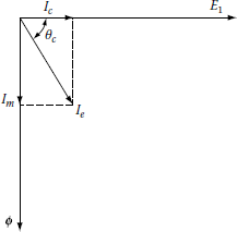
Figure 3.23 shows an approximate equivalent circuit with combined primary and reflected secondary and load impedances. Note that the secondary current I2 is seen by the primary side as I2/n and that the secondary and load impedances are transferred (or referred) to the primary side as n2(r2 + jxl2) and n2(RL + jXL), respectively. Also note that the secondary-side terminal voltage V2 is transferred as nV2.

Since the excitation current Ie is very small with respect to I2/n for a loaded transformer, the former may be ignored, as shown in Figure 3.24. Therefore, the equivalent impedance of the transformer referred to the primary is
Zeq=Z1+Z'2=Z1+n2Z2=req+jxeq(3.11)
where
Z1=r1+jxl2(3.12)
Z2=r2+jxl2(3.13)
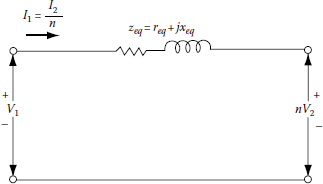
and therefore the equivalent resistance and the reactance of the transformer referred to the primary are
req=r1+n2r2(3.14)
and
xeq=xl1+n2xl2(3.15)
As before in Figure 3.25, for large-size power transformers,
req→0
therefore the equivalent impedance of the transformer becomes
Zeq=jxeq(3.16)
3.9 Single-Phase Transformer Connections
3.9.1 General
At present, the single-phase distribution transformers greatly outnumber the polyphase ones. This is partially due to the fact that lighting and the smaller power loads are supplied at single phase from single-phase secondary circuits. Also, most of the time, even polyphase secondary systems are supplied by single-phase transformers that are connected as polyphase banks.
Single-phase distribution transformers have one HV primary winding and two LV secondary windings that are rated at a nominal 120 V. Earlier transformers were built with four insulated secondary leads brought out of the transformer tank, the series or parallel connection being made outside the tank. Presently, in modern transformers, the connections are made inside the tank, with only three secondary terminals being brought out of the transformer.
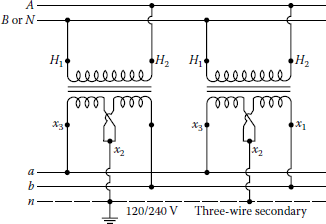
Single-phase distribution transformers have one HV primary winding and two LV secondary windings. Figure 3.26 shows various connection diagrams for single-phase transformers supplying single-phase loads. Secondary coils each rated at a nominal 120 V may be connected in parallel to supply a two-wire 120 V circuit, as shown in Figure 3.26a and b, or they may be connected in series to supply a three-wire 120/240 V single circuit, as shown in Figure 3.26c and d. The connections shown in Figure 3.26a and b are used where the loads are comparatively small and the length of the secondary circuits is short. It is often used for a single customer who requires only 120 V singlephase power.
However, for modern homes, this connection usually is not considered adequate. If a mistake is made in polarity when connecting the two secondary coils in parallel (see Figure 3.26a) so that the LV terminal 1 is connected to terminal 4 and terminal 2 to terminal 3, the result will be a shortcircuited secondary, which will blow the fuses that are installed on the HV side of the transformer (they are not shown in the figure). On the other hand, a mistake in polarity when connecting the coils in series (see Figure 3.26c) will result in the voltage across the outer conductors being zero instead of 240 V. Taps for voltage adjustment, if provided, are located on the HV winding of the transformer. Figure 3.26b and d shows single-bushing transformers connected to a multigrounded primary. They are used on 12,470 Gnd Y/7,200, 13,200 Gnd Y/7,620, and 24,940 Gnd Y/14,400 V multigrounded neutral systems. It is crucial that good and solid grounds are maintained on the transformer and on the system. Figure 3.27 shows single-phase transformer connections for singleand two-bushing transformers to provide customers who require only 240 V single-phase power. These connections are used for small industrial applications.
In general, however, the 120/240 V three-wire connection system is preferred since it has twice the load capacity of the 120 V system with only 12 times the amount of the conductor. Here, each 120 V winding has one-half the total kilovoltampere rating of the transformer. Therefore, if the connected 120 V loads are equal, the load is balanced, and no current flows in the neutral conductor. Thus the loads connected to the transformer must be held as nearly balanced as possible to provide the most economical usage of transformer capacity and to keep regulation to a minimum. Normally, one leg of the 120 V two-wire system and the middle leg of the 240 V two-wire or 120/240 V three-wire system are grounded to limit the voltage to ground on the secondary circuit to a minimum.
3.9.2 Single-Phase Transformer Paralleling
When greater capacity is required in emergency situations, two single-phase transformers of the same or different kilovoltampere ratings can be connected in parallel. The single-phase transformers can be of either additive or subtractive polarity as long as the following conditions are observed and connected, as shown in Figure 3.28:
- All transformers have the same turns ratio.
- All transformers are connected to the same primary phase.
- All transformers have identical frequency ratings.
- All transformers have identical voltage ratings.
- All transformers have identical tap settings.
- Per unit impedance of one transformer is between 0.925 and 1.075 of the other in order to maximize capability.
However, paralleling two single-phase transformers is not economical since the total cost and losses of two small transformers are much larger than one large transformer with the same capacity. Therefore, it should be used only as a temporary remedy to provide for increased demands for single-phase power in emergency situations. Figure 3.29 shows two single-phase transformers, each with two bushings, connected to a two-conductor primary to supply 120/240 V single-phase power on a three-wire secondary.
To illustrate load division among the parallel-connected transformers, consider the two transformers connected in parallel and feeding a load, as shown in Figure 3.30. Assume that the aforementioned conditions for paralleling have already been met (Figure 3.31).


Figure 3.21 shows the corresponding equivalent circuit referred to as the LV side. Since the transformers are connected in parallel, the voltage drop through each transformer must be equal. Therefore,
I1(Zeq,T1)=I2(Zeq,T2)(3.17)
from which
I1I2=Zeq,T2Zeq,T1(3.18)
where
I1 is the secondary current of transformer 1
I2 is the secondary current of transformer 2
IL is the load current
Zeq,1 is the equivalent impedance of transformer 1
Zeq,2 is the equivalent impedance of transformer 2
From Equation 3.18, it can be seen that the load division is determined only by the relative ohmic impedance of the transformers. If the ohmic impedances in Equation 3.18 are replaced by their equivalent in terms of percent impedance, the following equation can be found:
where
(%Z)T1 is the percent impedance of transformer 1
(%Z)T2 is the percent impedance of transformer 2
ST1 is the kilovoltampere rating of transformer 1
ST2 is the kilovoltampere rating of transformer 2
Equation 3.19 can be expressed in terms of kilovoltamperes supplied by each transformer since the primary and secondary voltages for each transformer are the same, respectively. Therefore,
where
SL1 is the kilovoltamperes supplied by transformer 1 to the load
SL2 is the kilovoltamperes supplied by transformer 2 to the load
Example 3.1
Figure 3.32 shows an equivalent circuit of a single-phase transformer with three-wire secondary for three-wire single-phase distribution. The typical distribution transformer is rated as 25 kVA, 7200-120/240 V, 60 Hz, and has the following per unit* impedance based on the transformer ratings and based on the use of the entire LV winding with zero neutral current:
and
An equivalent circuit of a single-phase transformer with three-wire secondary.
(From Lloyd, B., Electric Utility Engineering Reference Book-Distribution Systems, Vol. 3, Westinghouse Electric Corporation, East Pittsburgh, PA, 1965.)
Here, the two halves of the LV may be independently loaded, and, in general, the three-wire secondary load will not be balanced. Therefore, in general, the equivalent circuit needed is that of a three-winding single-phase transformer as shown in Figure 3.32, when voltage drops and/or fault currents are to be computed. Thus, use the meager amount of data (it is all that is usually available) and evaluate numerically all the impedances shown in Figure 3.32.
Solution
Figure 3.32 is based on the reference by Lloyd [1]. To determine approximately, Lloyd gives the following formula:
where is the transformer impedance referred to HV winding when the section of the LV winding between the terminals X2 and X3 is short-circuited.
From Figure 3.32, the turns ratio of the transformer is
Since the given per unit impedances of the transformer are based on the use of the entire LV winding,
Also, from Equation 3.21,
Therefore,
and
Example 3.2
Using the transformer equivalent circuit found in Example 3.1, determine the line-to-neutral (120 V) and line-to-line (240 V) fault currents in three-wire single-phase 120/240 V secondaries shown in Figures 3.33 and 3.34, respectively. In the figures, R represents the resistance of service-drop cable per conductor. Usually R is much larger than X for such cable and therefore X may be neglected.
Using the given data, determine the following:
- Find the symmetrical rms fault currents in the HV and LV circuits for a 120 V fault if R of the service-drop cable is zero.
- Find the symmetrical rms fault currents in the HV and LV circuits for a 240 V fault if R of the service-drop cable is zero.
- If the transformer is a CSPB type, find the minimum allowable interrupting capacity (in symmetrical rms amperes) for a circuit breaker connected to the transformer's LV terminals.
Solution
- When R = 0, from Figure 3.33, the line-to-neutral fault current in the secondary side of the transformer is
Thus the fault current in the HV side is
Note that the turns ratio is found as
- When R = 0, from Figure 3.24, the line-to-line fault current in the secondary side of the transformer is
Thus the fault current in the HV side is
Note that the turns ratio is found as
- Therefore, the minimum allowable interrupting capacity for a circuit breaker connected to the transformer LV terminals is 8181.7 A.
Example 3.3
Using the data given in Example 3.2, determine the following:
- Estimate approximately the value of R, that is, the service-drop cable’s resistance, which will produce equal line-to-line and line-to-neutral fault currents.
- If the conductors of the service-drop cable are aluminum, find the length of the servicedrop cable that would correspond to the resistance R found in part (a) in case of (1) #4 AWG conductors with a resistance of 2.58 Ω/mi and (2) #1/0 AWG conductors with a resistance of 1.03 Ω/mi.
Solution
- Since the line-to-line and the line-to-neutral fault currents are supposed to be equal to each other,
or
- The length of the service-drop cable is
- If #4 AWG aluminum conductors with a resistance of 2.58 Ω/mi or 4.886 × 10⁻⁴ Ω/ft are used,
- If #1/0 AWG aluminum conductors with a resistance of 1.03 Ω/mi or 1.9508 × 10⁻⁴ Ω/ft are used,
- If #4 AWG aluminum conductors with a resistance of 2.58 Ω/mi or 4.886 × 10⁻⁴ Ω/ft are used,
Example 3.4
Assume that a 250 kVA transformer with 2.4% impedance is paralleled with a 500 kVA transformer with 3.1% impedance. Determine the maximum load that can be carried without overloading either transformer. Assume that the maximum allowable transformer loading is 100% of the rating.
Solution
Designating the 250 and 500 kVA transformers as transformers 1 and 2, respectively, and using Equation 3.20,
Assume a load of 500 kVA on the 500 kVA transformer. The preceding result shows that the load on the 250 kVA transformer will be (0.6458) × (500 kVA) = 322.9 kVA when the load on the 500 kVA transformer is 500 kVA. Therefore, the 250 kVA transformer becomes overloaded before the 500 kVA transformer. The load on the 500 kVA transformer when the 250 kVA transformer is carrying rated load is
Thus the total load is
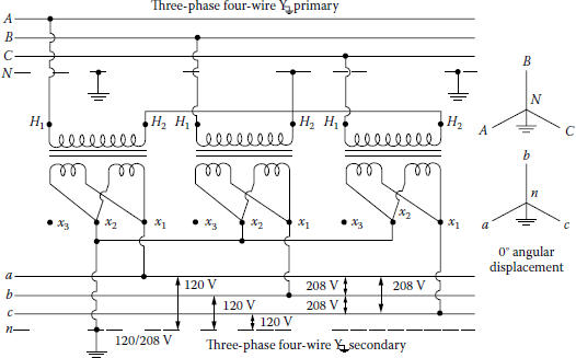
3.10 Three-Phase Connections
To raise or lower the voltages of three-phase distribution systems, either single-phase transformers can be connected to form three-phase transformer banks or three-phase transformers (having all windings in the same tank) are used. Figure 3.35 shows an eco-dry three-phase (resibloc) transformer. Figure 3.36 shows an air-to-water cooled resibloc three-phase transformer. Figure 3.37 shows an eco-dry (resibloc) three-phase transformer. Figure 3.38 shows a vacuum cast dry-type three-phase transformer.
Air-to-water cooled RESIBLOC three-phase transformer.
(Courtesy of ABB, Munich, Germany.)

Common methods of connecting three single-phase transformers for three-phase transformations are the delta–delta (Δ–Δ), wye–wye (Y–Y), wye–delta (Y–Δ), and delta–wye (Δ–Y) connections. Here, it is assumed that all transformers in the bank have the same kilovoltampere rating.
3.10.1 Δ–Δ Transformer Connection
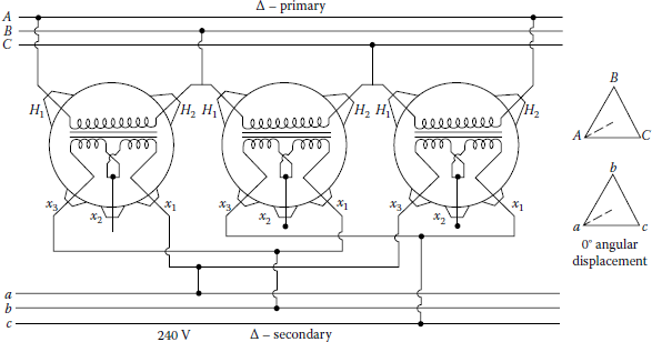
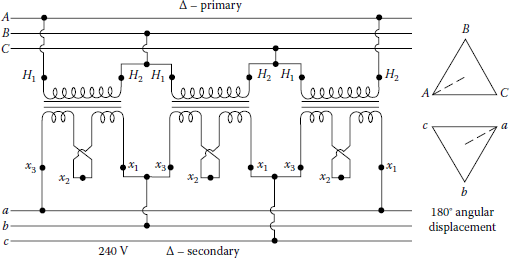
Figures 3.39 and 3.40 show the Δ–Δ connection formed by tying together single-phase transformers to provide 240 V service at 0° and 180° angular displacements, respectively.

This connection is often used to supply a small single-phase lighting load and three-phase power load simultaneously. To provide this type of service, the mid-tap of the secondary winding of one of the transformers is grounded and connected to the secondary neutral conductor, as shown in Figure 3.41. Therefore, the single-phase loads are connected between the phase and neutral conductors. Thus the transformer with the mid-tap carries two-thirds of the 120/240 V single-phase load and one-third of the 240 V three-phase load. The other two units each carry one-third of both the 120/240 and 240 V loads.

There is no problem from third-harmonic overvoltage or telephone interference. However, high circulating currents will result unless all three single-phase transformers are connected on the same regulating taps and have the same voltage ratios. The transformer bank rating is decreased unless all transformers have identical impedance values. The secondary neutral bushing can be grounded on only one of the three single-phase transformers, as shown in Figure 3.41.
Therefore, to get balanced transformer loading, the conditions include the following:
- All transformers have identical voltage ratios.
- All transformers have identical impedance values.
- All transformers are connected on identical taps.
However, if two of the units have the identical impedance values and the third unit has an impedance value that is within, plus or minus, 25% of the impedance value of the like transformers, it is possible to operate the Δ–Δ bank, with a small unbalanced transformer loading, at reduced bank output capacity. Table 3.5 gives the permissible amounts of load unbalanced on the odd and like transformers. Note that Z1 is the impedance of the odd transformer unit and Z2 is the impedance of the like transformer units. Therefore, with unbalanced transformer loading, the load values have to be checked against the values of the table so that no one transformer is overloaded.
Permissible Percent Loading on Odd and Like Transformers as a Function of the Z1/Z2 Ratio
% Load on |
||
Z1/Z2 Ratio |
Odd Unit |
Like Unit |
0.75 |
109.0 |
96.0 |
0.80 |
107.0 |
96.5 |
0.85 |
105.2 |
97.3 |
0.90 |
103.3 |
98.3 |
1.10 |
96.7 |
102.0 |
1.15 |
95.2 |
102.2 |
1.20 |
93.8 |
103.1 |
1.25 |
92.3 |
103.9 |
Assume that Figure 3.42 shows the equivalent circuit of a Δ–Δ-connected transformer bank referred to the LV side. A voltage-drop equation can be written for the LV windings as
where
Therefore, Equation 3.22 becomes
For the delta-connected secondary,
From Equation 3.24,
Adding the terms of and to either side of Equation 3.28 and substituting Equation 3.25 into the resultant equation,
and similarly,
and
If the three transformers shown in Figure 3.42 have equal percent impedance and equal ratios of percent reactance to percent resistance, then Equations 3.29 through 3.31 can be expressed as
where
ST,ab is the kilovoltampere rating of the single phase between phases a and b
ST,bc is the kilovoltampere rating of the single phase between phases b and c
ST,ca is the kilovoltampere rating of the single phase between phases c and a
Example 3.5
Three single-phase transformers are connected in Δ–Δ to provide power for a three-phase wyeconnected 200 kVA load with a 0.80 lagging power factor and an 80 kVA single-phase light load with a 0.90 lagging power factor, as shown in Figure 3.43.
Assume that the three single-phase transformers have equal percent impedance and equal ratios of percent reactance to percent resistance. The primary-side voltage of the bank is 7,620/13,200 V and the secondary-side voltage is 240 V. Assume that the single-phase transformer connected between phases b and c is rated at 100 kVA and the other two are rated at 75 kVA. Determine the following:
- The line current flowing in each secondary-phase wire
- The current flowing in the secondary winding of each transformer
- The load on each transformer in kilovoltamperes
- The current flowing in each primary winding of each transformer
- The line current flowing in each primary-phase wire
Solution
- (a) Using the voltage drop as the reference, the three-phase components of the line currents can be found as
Since the three-phase load has a lagging power factor of 0.80,
The single-phase component of the line currents can be found as
Since the single-phase load has a lagging power factor of 0.90, the current phasor lags its voltage phasor by –25.8°. Also, since the voltage phasor lags the voltage reference by 90° (see Figure 3.26), then the current phasor will lag the voltage reference by –115.8° (= –25.8° –90°). Therefore,
Hence, the line currents flowing in each secondary-phase wire can be found as
- (b) By using Equation 3.33, the current flowing in the secondary winding of transformer 1 can be found as
Similarly, by using Equation 3.32,
and using Equation 3.34,
- c. The kilovoltampere load on each transformer can be found as
- d. The current flowing in the primary winding of each transformer can be found by dividing the current flow in each secondary winding by the turns ratio. Therefore,
and hence
- e. The line current flowing in each primary-phase wire can be found as