
11.7 Series and Parallel Combinations
Simple combinations of series and parallel subsystems (or components) can be analyzed by successively reducing subsystems into equivalent parallel or series components.
Figure 11.17 shows a parallel–series system that has a high-level redundancy. The equivalent reliability of the system with m parallel paths of n components each can be expressed as
Rsys=1−(1−Rn)m(11.113)

where
Rsys is the equivalent reliability of system
Rn is the equivalent reliability of a path
R is the reliability of a component
n is the total number of components in a path
m is the total number of paths
Figure 11.18 shows a series–parallel system that has a low-level redundancy. The equivalent reliability of the system of n series units (or banks) with m parallel components in each unit (or bank) can be expressed as
Rsys=[1−(1−Rm)n](11.114)

where
Rsys is the equivalent reliability of system
1 – (1 – R)m is the equivalent reliability of a parallel unit (or bank)
R is the reliability of a component
m is the total number of components in a parallel unit (or bank)
n is the total number of units (or banks)
The comparison of the two systems shows that the series–parallel configuration provides higher system reliability than the equivalent parallel–series configuration for a given system. Therefore, it can be concluded that the lower the system level at which redundancy is applied, the larger the effective system reliability. The difference between parallel–series and series–parallel systems is not as pronounced if components have high reliabilities.
Example 11.4
Consider the various combinations of the reliability block diagrams shown in Figure 11.19. Assume that they are based on the logic diagrams of each subsystem and that the reliability of each component is 0.85. Determine the equivalent system reliability of each configuration.
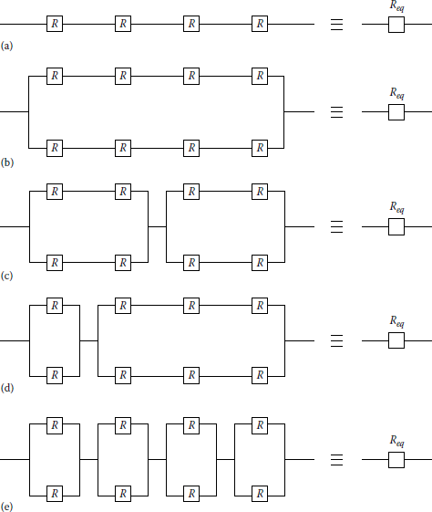
Various combinations of block diagrams: (a) series, (b) parallel–series, (c) mixed parallel, (d) mixed parallel, and (e) series–parallel.
Solution
- From Equation 11.63, the equivalent system reliability for the series system is
Req=Rsys = 4∏i=1Ri=(0.85)4=0.5220
- For the parallel–series system from Equation 11.113,
Req=1−(1−R4)2=1−[1−(0.85)4]2=0.7715
- For the mixed-parallel system,
Req=[1−(1−R2)2][1−(1−R2)2]=[1−(1−0.852)2][1−(1−0.852)2]=0.8519
- For the mixed-parallel system,
Req=[1−(1−R2)2][1−(1−R3)2]=[1−(1−0.852)2][1−(1−0.853)2]=0.8320
- For the series–parallel system from Equation 11.114,
Req=[1−(1−R2)]4=[1−(1−0.85)2]4=0.9130
Example 11.5
Assume that a system has five components, namely, A, B, C, D, and E, as shown in Figure 11.20, and that each component has different reliability as indicated in the figure. Determine the following:
- The equivalent system reliability.
- If the equivalent system reliability is desired to beat at least 0.80%, or 80%, design a system configuration to meet this system requirement by using each of the five components at least once.

Solution
- From Equation 11.63, the equivalent system reliability is
Req=5∏i=1Ri=(0.80)(0.95)(0.99)(0.90)(0.85)=0.4402 or 44.02%
- In general, the best way of improving the overall system reliability is to back the less-reliable components by parallel components. Therefore, since the relatively less-reliable components are λ and E, they can be backed by parallel redundancy as shown in Figure 11.21. Therefore, the new equivalent system reliability becomes
Rsys=5∏i=1Ri=[1−(1−0.80)2](0.95)(0.99)(0.90)[1−(1−0.65)4]=0.8004 or 80.04%

Example 11.6
Assume that a three-phase transformer bank consists of three single-phase transformers identified as A, B, and C for the sake of convenience. Assume that (1) transformer A is an old unit and therefore has a reliability of 0.90, (2) transformer B has been in operation for the last 20 years and therefore has been estimated to have a reliability of 0.95, and (3) transformer C is a brand new one with a reliability of 0.99. Based on the given information and assumption of independence, determine the following:
- The probability of having no failing transformer at any given time.
- If one out of the three transformers fails at any given time, what are the probabilities for that unit being the transformer A, or B, or C?
- If two out of the three transformers fail at any given time, what are the probabilities for those units being the transformers A and B, or B and C, or C and A?
- What is the probability of having all three transformers out of service at any given time?
Solution
- The probability of having no failing transformer at any given time is
P[A∩B∩C]=P(A)P(B)P(C)=(0.90)(0.95)(0.99)=0.84645
- If one out of the three transformers fails at any given time, the probabilities for that unit being the transformer A, or B, or C are
- If two out of the three transformers fail at any given time, the probabilities for those units being the transformers A and B, or B and C, or C and A are
- The probability of having all three transformers out of service at any given time* is
Therefore, the aforementioned reliability calculations can be summarized as given in Table 11.3.
11.8 Markov Processes*
A stochastic process, {X(t); t∈T}, is a family of random variables such that for each t contained in the index set T, X(t) is a random variable. Often T is taken to be the set of nonnegative integers.
In reliability studies, the variable t represents time, and X(t) describes the state of the system at time t. The states at a given time tn actually represent the (exhaustive and mutually exclusive) outcomes of the system at that time. Therefore, the number of possible states may be finite or infinite. For instance, the Poisson distribution
represents a stochastic process with an infinite number of states. If the system starts at time 0, the random variable n represents the number of occurrences between 0 and t. Therefore, the states of the system at any time t are given by n = 0, 1, 2....
A Markov process is a stochastic system for which the occurrence of a future state depends on the immediately preceding state and only on it. Because of this reason, the markovian process is characterized by a lack of memory. Therefore, a discrete parameter stochastic process, {X(t); t = 0, 1, 2,...}, or a continuous parameter stochastic process, {X(t); t ≥ 0}, is a Markov process if it has the following markovian property:
for any set of n time points, t1 < t2 < ··· tn in the index set of the process, and any real numbers x1, x2, .., xn. The probability of
is called the transition probability and represents the conditional probability of the system being in xn at tn, given it was xn–1 at tn–1. It is also called the one-step transition probability due to the fact that it represents the system between tn–1, and tn. One can define a k-step transition probability as
or as
A Markov chain is defined by a sequence of discrete-valued random variables, {X(tn)}, where tn is discrete-valued or continuous. Therefore, one can also define the Markov chain as the Markov process with a discrete state space. Define
as the one-step transition probability of going from state i at tn–1 to state j at tn and assume that these probabilities do not change over time. The term used to describe this assumption is stationarity. If the transition probability depends only on the time difference, then the Markov chain is defined to be stationary in time. Therefore, a Markov chain is completely defined by its transition probabilities, of going from state i to state j, given in a matrix form:
The matrix P is called a one-step transition matrix (or stochastic matrix) since all the transition probabilities pij’s are fixed and independent of time. The matrix P is also called just the transition matrix when there is no possibility of confusion. Since the pij’s are conditional probabilities, they must satisfy the conditions
and
where
i = 0, 1, 2,..., n
j = 0,1, 2,..., n
Note that when the number of transitions (or states) is not too large, the information in a given transition matrix P can be represented by a transition diagram. The transition diagram is a pictorial map of the process in which states are represented by nodes and transitions by arrows. Here, the focus is not on time but on the structure of allowable transitions. The arrow from node i to node j is labeled as pij. Since row i of the matrix P corresponds to the set of arrows leaving node i, the sum of their probabilities must be equal to unity.
Assume that a given system has two states, namely, state 1 and state 2. For example, here, states 1 and 2 may represent the system being up and down, respectively. Therefore, the associated transition probabilities can be defined as
p11 = probability of being in state 1 at time t, given that it was in state 1 at time zero
p12 = probability of being in state 2 at time t, given that it was in state 2 at time zero
p21 = probability of being in state 2 at time t, given that it was in state 1 at time zero
p22 = probability of being in state 1 at time t, given that it was in state 2 at time zero
Therefore, the associated transition matrix can be expressed as
Figure 11.22a shows the associated transition diagram.

By the same token, if the given system has three states, its transition matrix can be expressed as
and its transition diagram can be drawn as shown in Figure 11.22b.
Example 11.7
Based on past history, a distribution engineer of the NL&NP Company has gathered the following information on the operation of the distribution transformers served by the Riverside Substation. The records indicate that only 2% of the transformers that are presently down and therefore being repaired now will be down and therefore will need repair next time. The records also show that 5% of those transformers that are currently up and therefore in service now will be down and therefore will need repair next time. Assuming that the process is discrete, markovian, and has stationary transition probabilities, determine the following:
- The conditional probabilities
- The transition matrix
- The transition diagram
Solution
- Let t and t + 1 represent the present time (i.e., now) and the next time, respectively. Therefore, the associated conditional probabilities are
- Let numbers 1 and 2 represent the states of down and up, respectively. Therefore, from Equation 11.120 and part a,
or, from Equation 11.121,
- Therefore, the transition diagram can be drawn as shown in Figure 11.23.

Example 11.8
Assume that a distribution engineer of the NL&NP Company has studied the feeder outage statistics of the troublesome Riverside Substation and found out (1) that there is a markovian relationship between the feeder outages occurring at the present time and the next time and (2) that the relationship is a stationary one. Assume that the engineer has summarized the findings as shown in Table 11.4. For example, the table shows that if the presently outaged feeder is number 1, then the chances for the next outaged feeder being feeder 1, 2, or 3 are 40%, 30%, and 30%, respectively. Using the given data, determine the following:
- The conditional outage probabilities
- The transition matrix
- The transition diagram
Feeder Outage Data
Presently Outaged Feeder |
Chances, in Percent, for the Next Outaged Feeder Being |
||
|---|---|---|---|
1 |
2 |
3 |
|
1 |
40 |
30 |
30 |
2 |
20 |
50 |
30 |
3 |
25 |
25 |
50 |
Solution
- Let t and t + 1 represent the present time and the next time, respectively. Therefore, the probability of the next outaged feeder being number 1, given it is number 1 now, can be expressed as
where
Xt+1 is the outaged feeder at next time
Xt is the outaged feeder at present time
Similarly,
- Therefore, the transition matrix is
- The associated transition diagram is shown in Figure 11.24.

11.8.1 Chapman-Kolmogorov Equations
Assume that Sj represents the exhaustive and mutually exclusive states (outcomes) of a given system at any time, where j = 0, 1, 9,.... Also assume that the system is markovian and that represents the absolute probability that the system is in state Sj at t0. Therefore, if and the transition matrix P of a given Markov chain are known, one can easily determine the absolute probabilities of the system after n-step transitions. By definition, the one-step transition probabilities are
Therefore, the n-step transition probabilities can be defined by induction as
In other words, is the probability (absolute probability) that the process is in state j at time tn, given that it was in state i at time t0. It can be observed from this definition that must be 1 if i = j, and 0 otherwise.
The Chapman–Kolmogorov equations provide a method for computing these n-step transition probabilities. In general form, these equations are given as
for any m between zero and n. Note that Equation 11.128 can be represented in matrix form by
Therefore, the elements of a higher-order transition matrix, that is, , can be obtained directly by matrix multiplication. Hence,
Note that a special case of Equation 11.128 is
and therefore, the special cases of Equations 11.129 and 11.130 are
and
respectively.
The unconditional probabilities such as
are called the absolute probabilities or state probabilities. To determine the state probabilities, the initial conditions must be known. Therefore,
Note that Equation 11.135 can be represented in matrix form by
where
p(n) is the vector of state probabilities at time tn
p(0) is the vector of initial state probabilities at time t0
P(n) is the n-step transition matrix
The state probabilities or absolute probabilities are defined in vector form as
and
Example 11.9
Consider a Markov chain, with two states, having the one-step transition matrix of
and the initial state probability vector of
and determine the following:
- The vector of state probabilities at time t1
- The vector of state probabilities at time t4
- The vector of state probabilities at time t8
Solution
- From Equation 11.136,
- From Equation 11.136,
where
and thus,
Therefore
- From Equation 11.136,
where
Therefore,
Here, it is interesting to observe that the rows of the transition matrix P(8) tend to be the same. Furthermore, the state probability vector p(8) tends to be the same with the rows of the transition matrix P(8). These results show that the long-run absolute probabilities are independent of the initial state probabilities, that is, p(0). Therefore, the resulting probabilities are called the steady-state probabilities and defined as the set of πj, where
In general, the initial state tends to be less important to the n-step transition probability as n increases, such that
so that one can get the unconditional steady-state probability distribution from the n-step transition probabilities by taking n to infinity without taking the initial states into account. Therefore,
or
and thus,
where
Note that the matrix has identical rows so that each row is a row vector of
Since the transpose of a row vector Π is a column vector Πt, Equation 11.143 can also be expressed as
which is a set of linear equations.
To be able to solve equation sets (11.143) or (11.146) for individual πi’s, one additional equation is required. This equation is called the normalizing equation and can be expressed as
11.8.2 Classification of States in Markov Chains
Two states i and j are said to communicate, denoted as i ~ j, if each is accessible (reachable) from the other, that is, if there exists some sequence of possible transitions that would take the process from state i to state j.
A closed set of states is a set such that if the system, once in one of the states of this set, will stay in the set indefinitely; that is, once a closed set is entered, it cannot be left. Therefore, an ergodic set of states is a set in which all states communicate and which cannot be left once it is entered. An ergodic state is an element of an ergodic set. A state is called transient if it is not ergodic. If a single state forms a closed set, the state is called an absorbing state. Thus, a state is an absorbing state if and only if pij = 1.
11.9 Development of the State-Transition Model to Determine the Steady-State Probabilities
The Markov technique can be used to determine the steady-state probabilities. The model given in this section is based on the zone-branch technique developed by Koval and Billinton [11,12].
Assuming the process given in a markovian model is irreducible and all states are ergodic, one can derive a set of linear equations to determine the steady-state probabilities as
Therefore, for example, the system differential equations can be expressed in the matrix form for a single-component state as [13]
where
λ is the normal weather failure rate of component
μ is the normal weather repair rate of component
μ' is the adverse weather failure rate of component
μ' is the adverse weather repair rate of component
Also,
and
where
N is the expected duration of normal weather period
S is the expected duration of adverse weather period
Equation 11.148 can be expressed in the matrix form as
where
[dP(t)/dt] is the matrix whose (i, j)th element is dpij(t)/dt
P(t) is the matrix whose (i, j)th element is pij(t)
Λ is the matrix whose (i, j)th element is λij
Also, each element in matrix equation (11.152) can be expressed as
or
since
or
However, since the differentiation of a constant is zero, that is,
Equation 11.157 becomes
or, in the matrix form,
where
0 is the row vector of zeros
Λ is the matrix of transition rates
Π is the row vector of steady-state probabilities
Since the equations in the matrix equation (11.160) are dependent, introduction of an additional equation is necessary, that is,
which is called the normalizing equation.
The matrix Λ can be expressed as
where
λij = −di for i = j, called the rate of departure from state i
λij = eij for i ≠ j, called the rate of entry from state i to state j
Therefore, matrix equation (11.162) can be reexpressed as
Likewise,
Therefore, substituting Equations 11.163 and 11.164 into Equation 11.160,
or
Therefore,
or
Also,
or
As Koval and Billinton [11,12] suggested, once the long-term or steady-state probabilities of each state are computed from Equations 11.168 to 11.170, one can readily calculate the total failure rate and the average repair rate of the particular zone i and branch j. These rates also take into consideration the effects of interruptions on other parts of the system. The total failure rate of zone i branch j is given by Koval and Billinton [11] as
where
λij is the total failure rate of zone branch ij
λs is the failure rate of supply, that is, feeding substation
RIA(ij, k) is the recognition and isolation array coefficients,
I is the failed zone-branch array coefficient = FZB(k)
Likewise, the average downtime, that is, repair time, for each zone i branch j is given as
or
where
rij is the average repair time for each zone i branch j
is the downtime array coefficients
I is the failed zone-branch array coefficient, = FZB(k)
11.10 Distribution Reliability Indices
Since a typical distribution system accounts for 40% of the cost to deliver power and 80% of customer reliability problems, distribution system design and operation is critical for financial success of the utility company and customer satisfaction.
Interruptions and outages can be studied through the use of predictive reliability assessment tools that can predict customer reliability characteristics based on system topology and component reliability data. In order to achieve this, distribution reliability indices are calculated. Such reliability indices should be concerned with both duration and frequency of outage.
They also need to consider overall system conditions as well as specific customer conditions. Using averages all lead to loss of some information such as time until the last customer is returned to service, but averages should give a general trend of conditions for the utility.
Here, it is assumed that as seen as the customer service interrupted, the crews are dispatched and the restoration work starts immediately. Therefore, the duration of interruption is the same as the duration of restoration.
11.11 Sustained Interruption Indices
These indices are also known as customer-based indices.
11.11.1 SAIFI
System average interruption frequency index (SAIFI) (sustained interruptions). This index is designed to give information about the average frequency of sustained interruptions per customer over a predefined area. Therefore,
or
where
Ni is the number of interrupted customers for each interruption event during reporting period
NT is the total number of customers served for the area being indexed
11.11.2 SAIDI
System average interruption duration index (SAIDI). This index is commonly referred to as customer minutes of interruption or customer hours, and is designed to provide information about the average time the customers are interrupted. Thus,
or
where
ri is the restoration time for each interruption event.
11.11.3 CAIDI
Customer average interruption duration index (CAIDI). It represents the average time required to restore service to the average customer per sustained interruption. Hence,
or
11.11.4 CTAIDI
Customer total average interruption duration index (CTAIDI). For customers who actually experienced an interruption, this index represents the total average time in the reporting period they were without power. This index is a hybrid of CAID and is calculated the same except that customers with multiple interruptions are counted only once. Therefore,
or
where CN is total number of customers who have experienced a sustained interruption during the reporting period.
In tallying total number of customers interrupted, each individual customer should only be counted once regardless of the number of times interrupted during the reporting period. This applies to both CTAIDI and CAIFI.
11.11.5 CAIFI
Customer average interruption frequency index (CAIFI). This index gives the average frequency of sustained interruptions for those customers experiencing sustained interruptions. The customer is counted only once regardless of the number of times interrupted. Thus,
or
11.11.6 ASAI
Average service availability index (ASAI). This index represents the fraction of time (often in percentage) that a customer has power provided during 1 year or the defined reporting period. Hence,
or
There are 8760 h in a regular year, 8784 in a leap year.
11.11.7 ASIFI
Average system interruption frequency index (ASIFI). This index was specifically designed to calculate reliability based on load rather than number of customers. It is an important index for areas that serve mainly industrial/commercial customers.
It is also used by utilities that do not have elaborate customer tracking systems. Similar to SAIFI, it gives information on the system average frequency of interruption. Therefore,
or
where
is the total connected kVA load interrupted for interruption event
LT is the total connected kVA load served
11.11.8 ASIDI
Average system interruption duration index (ASIDI). This index was designed with the same philosophy as ASIFI, but it provides information on system average duration of interruptions. Thus,
or
11.11.9 CEMIn
Customers experiencing multiple interruptions (CEMIn). This index is designed to track the number n of sustained interruptions to a specific customer. Its purpose is to help identify customer trouble that cannot be seen by using averages. Hence,
or
where CN(k>n) is the total number of customers who have experienced more than n sustained interruptions during the reporting period.
11.12 Other Indices (Momentary)
11.12.1 MAIFI
Momentary average interruption frequency index (MAIFI). This index is very similar to SAIFI, but it tracks the average frequency of momentary interruptions. Therefore,
or
where IDi is the number of interrupting device operations.
MAIFI is the same as SAIFI, but it is for short-duration rather than long-duration interruptions.
11.12.2 MAIFIE
Momentary average interruption event frequency index (MAIFIE). This index is very similar to SAIFI, but it tracks the average frequency of momentary interruption events. Thus,
or
where IDE is the interrupting device events during reporting period.
Here, Ni is the number of customers experiencing momentary interrupting events. This index does not include the events immediately preceding a lockout.
Momentary interruptions are most commonly tracked by using breaker and recloser counts, which implies that most counts of momentaries are based on MAIFI and MAIFIE. To accurately count MAIFIE, a utility must have a supervisory control and data acquisition (SCADA) system or other time-tagging recording equipment.
11.12.3 CEMSMIn
Customers experiencing multiple sustained interruption and momentary interruption events (CEMSMIn). This index is designed to track the number n of both sustained interruption and momentary interruption events to a set of specific customers.
Its purpose is to help identify customer trouble that cannot be seen by using averages. Hence,
or
where CNT(k>n) is the total number of customers who have experienced more than n sustained interruption and momentary interruption events during the reporting period.
11.13 Load- and Energy-Based Indices
There are also load- and energy-based indices. In determination of such indices, one has to know the average load at each load bus. This average load Lavg at a bus is found from
where
Lavg is the peak load (demand)
FLD is the load factor
The average load can also be found from
If the period of interest is a year,
11.13.1 ENS
Energy not supplied index (ENS). This index represents the total energy not supplied by the system and is expressed as
where Lavg,i is the average load connected to load point i.
11.13.2 AENS
Average energy not supplied (AENS). This index represents the average energy not supplied by the system.
or
This index is the same as the average system curtailment index (ASCI).
11.13.3 ACCI
Average customer curtailment index (ACCI). This index represents the total energy not supplied per affected customer by the system.
or
It is a useful index for monitoring the changes of average energy not supplied between one calendar year and another.
Example 11.10
The Ghost Town Municipal Electric Utility Company (GMEU) has a small distribution system for which the information is given in Tables 11.5 and 11.6. Assume that the duration of interruption is the same as the restoration time. Determine the following reliability indices:
- SAIFI
- CAIFI
- SAIDI
- CAIDI
- ASAI
- ASIDI
- ENS
- AENS
- ACCI
Distribution System Data of GMEU Company
Load Point |
Number of Customers (Ni) |
Average Load Connected (kW) (Lavg,i) |
|---|---|---|
1 |
250 |
2,300 |
2 |
300 |
3,700 |
3 |
200 |
2,500 |
4 |
250 |
1,600 |
—— |
—— |
|
NT = 1,000 |
LT = 10,100 |
Solution
-
Annual Interruption Effects
Load Point Affected
Number of Customers Load Interrupted (Ni)
Load Interrupted (kW) (Li)
1
250
2,300
2
200
2,500
3
250
1,600
4
250
1,600
——
——
950
8,000
Load Point Affected
Duration of Interruptions (h) (di = ri)
Customer Hours Curtailed (ri × Ni)
Energy Not Supplied (kWh) (ri × Li)
1
2
500
4,600
2
3
600
7,500
3
1
250
1,600
4
1
250
1,600
——
——
1,600
15,300
CN, number of customers affected = 250 + 200 + 250 = 700.
11.14 Usage of Reliability Indices
Based on the two industry-wide surveys, the Working group on System Design of IEEE Power Engineering Society’s T&D Subcommittee has determined that the most commonly used indices are SAIDI, SAIFI, CAIDI, and ASAI in the descending popularity order of 70%, 80%, 66.7%, and 63.3%, respectively. Most utilities track one or more of the reliability indices to help them understand how the distribution system is performing.
For example, removing the instantaneous trip from the substation recloser has an effect on the whole circuit. The first area to look at is the effect on the reliability indices. With the advent of the digital clock and electronic equipment, a newer index (i.e., MAIFI, which tracks momentary outages) is gaining in popularity.
With the substation recloser instantaneous trip on, the SAIDI and CAIDI indices should be low, due to the “fuse saving” effect when clearing momentary faults. The MAIFI, however, will be high due to the blinks on the whole circuit. By removing the instantaneous trip, the MAIFI should be reduced but the SAIDI will increase.
11.15 Benefits of Reliability Modeling in System Performance
A reliability assessment model quantifies reliability characteristics based on system topology and component reliability data. The aforementioned reliability indices can be used to assess the past performance of a distribution system. Assessment of system performance is valuable for various reasons.
For example, it establishes the changes in system performance and thus helps to identify weak areas and the need for reinforcement. It also identifies overloaded and undersized equipment that degrades system reliability. Also, it establishes existing indices that can be used in the future reliability assessments. It enables previous predictions to be compared with actual operating experience. Such results can benefit many aspects of distribution planning, engineering, and operations. Reliability problems associated with expansion plans can be predicted.
However, a reliability assessment study can help to quantify the impact of design improvement options. Adding a recloser to a circuit will improve reliability, but by how much? Reliability models answer this question. Typical improvement options that can be studied based on a predictive reliability model include the following:
- New feeders and feeder expansions
- Load transfers between feeders
- New substation and substation expansions
- New feeder tie points
- Line reclosers
- Sectionalizing switches
- Feeder automation
- Replacement of aging equipment
- Replacing circuits by underground cables
According to Brown [22], reliability studies can help to identify the number of sectionalizing switches that should be placed on a feeder, the optimal location of devices, and the optimal ratings of new equipment. Adding a tie switch may reduce index by 10 min, and reconductoring for contingencies may reduce SAIDI by 5 min. Since reconductoring permits the tie switch to be effective, doing both projects may result in a SAIDI reduction of 30 min, doubling the cost-effectiveness of each project.
Cost-effectiveness is determined by computing the cost of each reliability improvement option and computing a benefit/cost ratio. This is a measure of how much reliability is purchased with each dollar being spent. Once all projects are ranked in order of cost-effectiveness, projects and project combinations can be approved in order of descending cost-effectiveness until reliability targets are met or budget constraints become binding. This process is referred to as value-based planning and engineering. In a given distribution system, reliability improvements can be achieved by various means, which include the following [22]:
- Increased line sectionalizing: It is accomplished by placing normally closed switching devices on a feeder. Adding fault interrupting devices (fuses and reclosers) improves devices by reducing the number of customers interrupted by downstream faults. Adding switches without fault interrupting capability improves reliability by permitting more flexibility during post-fault system reconfiguration.
- New tie points: A tie point is a normally open switch that permits a feeder to be connected to an adjacent feeder. Adding new tie points increases the number of possible transfer paths and may be a cost-effective way to improve reliability on feeders with low transfer capability.
- Capacity constrained load transfers: Following a fault, operators and crews can reconfigurate a distribution system to restore power to as many customers as possible. Reconfiguration is only permitted if it does not load a piece of equipment above its emergency rating. If a load transfer is not permitted because it will overload a component, the component is charged with a capacity constraint. System reliability is reduced, because the equipment does not have sufficient capacity for reconfiguration to take place.
- Transfer path upgrades: A transfer path is an alternate path to serve load after a fault takes place. If a transfer path is capacity constrained due to small conductor sizes, reconductoring may be a cost-effective way to improve reliability.
- Feeder automation: SCADA-controlled switches on feeders permit post-fault system reconfiguration to take place much more quickly than with manual switches, permitting certain customers to experience a momentary interruption rather than a sustained interruption.
In summary, distribution system reliability assessment is crucial in providing customers more with less cost. Today, computer softwares are commercially available, and the time has come for utilities to treat reliability issues with the same analytical rigor as capacity issues.
11.16 Economics of Reliability Assessment
Typically, as investment in system reliability increases, the reliability improves, but it is not a linear relationship. By calculating the cost of each proposed improvement and finding a ration of the increased benefit to the increased cost, the cost-effectiveness can be quantified.
Once the cost-effectiveness of the improvement options has been quantified, they can be prioritized for implementation. This incremental analysis of how reliability improves and affects the various indices versus the additional cost is necessary in order to help ensure that scarce resources are used most effectively.
Quantifying the additional cost of improved reliability is important, but additional considerations are needed for a more complete analysis. The costs associated with an outage are placed side by side against the investment costs for comparison in helping to find the true optimal reliability solution. Outage costs are generally divided between utility outage costs and customer outage costs.
Utility outage costs include the loss of revenue for energy not supplied, and the increased maintenance and repair costs to restore power to the customers affected. According to Billinton and Wang [23], the maintenance and repair costs can be quantified as
where
Ci is the labor cost for each repair and maintenance action, in dollars
Ccomp is the component replacement or repair costs, in dollars
Therefore, the total utility cost for an outage is
While the outage costs to the utility can be significant, often the costs to the customer are far greater. These costs vary greatly by customer sector type and geographical location. Industrial customers have costs associated with loss of manufacture, damaged equipment, extra maintenance, loss of products and/or supplies to spoilage, restarting costs, and greatly reduced worker productivity effectiveness.
Commercial customers may lose business during the outage and experience many of the same losses as industrial customers, but on a possibly smaller scale.
Residential customers typically have costs during a given outage that are far less than the previous two, but food spoilage, loss of heat during winter, or air conditioning during a heat wave can be disproportionately large for some individual customers. In general, customer outage costs are more difficult to quantify. Through collection of data from industry and customer surveys, a formulation of sector damage functions is derived, which lead to composite damage functions.
According to Lawton et al. [24], the sector customer damage function (SCDF) is a cost function of each customer sector. The composite customer damage function (CCDF) is an aggregation of the SCDF at specified load points and is weighted proportionally to the load at the load points. For n customers,
where Ci is the energy demand of customer type i.
Therefore, the customer outage cost by sector is
where Li is the average load at load point i.
Since the CCDF is a function of outage attributes, customer characteristics, and geographical characteristics, it is important to have accurate information about these variables. Although outage attributes include duration, season, time of day, advance notice, and day of the week, the most heavily weighted factor is outage duration.
The total customer cost for all applicable sectors can be found for a particular load point from
or
However, using the CCDF marks the outage cost that is borne disproportionately by the different sectors. For a reliability planning, in addition to the load point indices of λ, r, and U, one has to determine the following reliability cost/worth indices [23]:
- Expected energy not supplied (EENS) index: It is defined as
where
Ne is the total number of elements in the distribution system
Li is the average load at load point i
rij is the failure duration at load point i due to component j
λij is the failure rate at load point i due to component j
- Expected customer outage cost (ECOST) index: It is defined
where SCDFij is the sector customer damage function at load point i due to component j
- Interrupted energy assessment rate (IEAR) indices: It is defined as
This index provides a quantitative worth of the reliability for a particular load point in terms of cost for each unit of energy not supplied.
The reliability cost/worth analysis provides a more comprehensive analysis of the time reliability cost of the system. In addition to the incentives for improving the system indices and keeping system costs under control, costs help to ensure that the reliability investment costs are apportioned judiciously for maximum benefit to both the utility and the end user.
Reliability is terribly important for the customer. In one study performed in the Eastern United States in 2002, the “average” residential customer cost for an outage duration of 1 h was approximately $3, for a small-to-medium commercial customer the cost was $1,200, and for a large industrial customer the cost was $82,000 [24]. Providing a comprehensive reliability cost/worth assessment is a tool in order to help ensure a reliable electricity supply is available and that the system costs of the utility company are well justified.
Problems
- 11.1 Assume that the given experiment is tossing a coin three times and that a single outcome is defined as a certain succession of heads (H) and tails (T), for example, (HHT).
- How many possible outcomes are there? Name them.
- What is the probability of tossing three heads, that is, (HHH)?
- What is the probability of getting heads on the first two tosses?
- What is the probability of getting heads on any two tosses?
- 11.2 Two cards are drawn from a shuffled deck. What is the probability that both cards will be aces?
- 11.3 Two cards are drawn from a shuffled deck.
- What is the probability that two cards will be the same suit?
- What is the probability if the first card is replaced in the deck before the second one is drawn?
- 11.4 Assume that a substation transformer has a constant hazard rate of 0.005 per day.
- What is the probability that it will fail during the next 5 years?
- What is the probability that it will not fail?
- 11.5 Consider the substation transformer in Problem 11.4 and determine the probability that it will fail during year 6, given that it survives 5 years without any failure.
- 11.6 What is the MTTF for the substation transformer of Problem 11.4?
- 11.7 Determine the following for a parallel connection of three components:
- The reliability
- The availability
- The MTTF
- The frequency
- The hazard rate
- 11.8 A large factory of the International Zubits Company has 10 identical loads that switch on and off intermittently and independently with a probability p of being “on.” Testing of the loads over a long period has shown that, on the average, each load is on for a period of 12 min/h. Suppose that when switched on, each load draws some X kVA from the Ghost River Substation that is rated 7X kVA. Find the probability that the substation will experience an overload. (Hint: Apply the binomial expansion.)
- 11.9 Verify Equation 11.79.
- 11.10 Verify Equation 11.83.
- 11.11 Using Equation 11.78, derive and prove that the mean time to repair a two-component system is
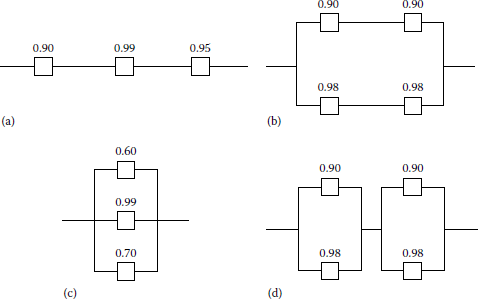
- 11.12 Calculate the equivalent reliability of each of the system configurations in Figure P11.12, assuming that each component has the indicated
- 11.13 Calculate the equivalent reliability of each of the system configurations in Figure P11.13, assuming that each component has the indicated reliability.
- 11.14 Determine the equivalent reliability of the system in Figure P11.14.
- 11.15 Using the results of Example 11.6, determine the following:
- The probability of having any one of the three transformers out of service at any given time.
- The probability of having any two of the three transformers out of service at any given time.
- 11.16 Using the results of Example 11.6, determine the following:
- The probability of having at least one of the three transformers out of service at any given time.
- The probability of having at least two of the three transformers out of service at any given time.
- 11.17 Repeat Example 11.2, assuming that the underground section of the feeder has been increased another mile due to growth in the downtown area and that on the average, the annual fault rate of the underground section has increased to 0.3 due to the growth and aging.
- 11.18 Repeat Example 11.3 for customers D–F, assuming that they all exist as shown in Figure 11.16.
- 11.19 Repeat Problem 11.18 but assume that during emergency the end of the existing feeder can be connected to and supplied by a second feeder over a normally open tie breaker.
- 11.20 Verify Equation 11.172 for a two-component system.
- 11.21 Verify Equation 11.172 for an n-component system.
- 11.22 Derive Equation 11.131 based upon the definition of n-step transition probabilities of a Markov chain.
- 11.23 Use the data given in Example 11.8 and assume that feeder 1 has just had an outage. Using the joint probability concept of the classical probability theory techniques and the system’s probability tree diagram, determine the probability that there will be an outage on feeder 2 at the time after the next outage.
- 11.24 Repeat Problem 11.23 by using the Markov chains concept rather than the classical probability theory techniques.
- 11.25 Use the data given in Example 11.8 and the Markov chains concept. Assuming that there is an outage on feeder 3 at the present time, determine the following:
- The probabilities of being in each of the respective states at time t1.
- The probabilities of being in each of the respective states at time t2.
- 11.26 Use the data given in Example 11.8 and the Markov chains concept. Assume that there is an outage on feeder 2 at the present time and determine the probabilities associated with this outage at time t4.
- 11.27 Use the data given in Example 11.8 and the Markov chains concept. Determine the complete outage probabilities at time t4.
- 11.28 Derive Equation 11.187 from Equation 11.186.
- 11.29 Consider a radial feeder supplying three laterals and assume that the distribution system data and annual interruption effects of a utility company are given in Tables P11.29A and B, respectively. Assume that the duration of interruption is the same as the restoration time. Determine the following reliability indices:
- SAIFI
- CAIFI
- SAIDI
- CAIDI
- ASAI
- ASIDI
- ENS
- AENS
- ACCI
Distribution System Data
Load Point
Number of Customers (Ni)
Average Load Connected (kW) (Lavg,i)
1
1800
8400
2
1300
6000
3
900
4600
—
—
NT = 4000
LT = 1900
Annual Interruption Effects
Load Point Affected
Number of Customers Load Interrupted (Ni)
Load Interrupted (kW) (Li)
2
800
3,600
3
600
2,800
3
300
1,800
3
600
2,800
2
500
2,400
3
300
1,800
—
—
3100
15,200
Load Point Affected
Duration of Interruptions (h) (di = ri)
Customer Hours Curtailed (ri × Ni)
Energy Not Supplied (kWh) (ri × Li)
2
3
2400
10,800
3
3
1800
8,400
3
2
600
3,600
3
1
600
2,800
2
1.5
750
3,600
3
1.5
450
2,700
—
—
6,600
31,900
CN, number of customers affected = 800 + 600 + 350 + 500 = 2,200.
- 11.30 Assume that a radial feeder is made up of three sections (i.e., sections A, B, and C) and that a load is connected at the end of each section. Therefore, there are three loads, that is, L1, L2, and L3. Table P11.30A gives the component data for the radiai feeder. Table P11.30B gives the load point indices for the radiai feeder. Finally, Table P11.30C gives the distribution system data. Determine the following reliability indices:
- 11.31Resolve Example 11.3 by using MATLAB. Assume that all the quantities remain the same.
- 11.32Resolve Example 11.9 by using MATLAB.


References
1. IEEE Committee Reports: Proposed definitions of terms for reporting and analyzing outages of electrical transmission and distribution facilities and interruptions, IEEE Trans. Power Appar. Syst., 87, May 5, 1968, 1318–1323.
2. Endrenyi, J.: Reliability Modeling in Electric Power Systems, Wiley, New York, 1978.
3. IEEE Committee Report: Definitions of customer and load reliability indices for evaluating electric power performance, Paper A75 588-4, presented at the IEEE PES Summer Meeting, San Francisco, CA, July 20–25, 1975.
4. IEEE Committee Report: List of transmission and distribution components for use in outage reporting and reliability calculations, IEEE Trans. Power Appar. Syst., PAS-95(4), July/August 1976, 1210–1215.
5. Smith, C. O.: Introduction to Reliability in Design, McGraw-Hill, New York, 1976.
6. The National Electric Reliability Study: Technical Study Reports, U.S. Department of Energy DOE/ EP-0005, April 1981.
7. The National Electric Reliability Study: Executive Summary, U.S. Department of Energy, DOE/EP-0003, April 1981.
8. Billinton, R.: Power System Reliability Evaluation, Gordon and Breach, New York, 1978.
9. Albrect, P. F.: Overview of power system reliability, Workshop Proceedings: Power System Reliability- Research Needs and Priorities, EPRI Report WS-77-60, Palo Alto, CA, October 1978.
10. Billinton, R., R. J. Ringlee, and A. J. Wood: Power-System Reliability Calculations, M.I.T., Cambridge, MA, 1973.
11. Koval, D. O. and R. Billinton: Evaluation of distribution circuit reliability, Paper F77 067-2, IEEE PES Winter Meeting, New York, NY, January–February 1977.
12. Koval, D. O. and R. Billinton: Evaluation of elements of distribution circuit outage durations, Paper A77 685-1, IEEE PES Summer Meeting, Mexico City, Mexico, July 17–22, 1977.
13. Billinton, R. and M. S. Grover: Quantitative evaluation of permanent outages in distribution systems, IEEE Trans. Power Appar. Syst., PAS-94, May/June 1975, 733–741.
14. Gönen, T. and M. Tahani: Distribution system reliability analysis, Proceedings of the IEEE MEXICON-80 International Conference, Mexico City, Mexico, October 22–25, 1980.
15. Standard Definitions in Power Operations Terminology Including Terms for Reporting and Analyzing Outages of Electrical Transmission and Distribution Facilities and Interruptions to Customer Service, IEEE Standard 346–1973, 1973.
16. Heising, C. R.: Reliability of electrical power transmission and distribution equipment, Proceedings of the Reliability Engineering Conference for the Electrical Power Industry, Seattle, WA, February 1974.
17. Electric Power Research Institute: Analysis of Distribution R&D Planning, EPRI Report 329, Palo Alto, CA, October 1975.
18. Howard, R. A.: Dynamic Probabilistic Systems, Vol. I: Markov Models, Wiley, New York, 1971.
19. Markov, A.: Extension of the limit theorems of probability theory to a sum of variables connected in a chain, Izv. Akad. Nauk St. Petersburg (translated as Notes of the Imperial Academy of Sciences of St. Petersburg), December 5, 1907.
20. Gönen, T. and M. Tahani: Distribution system reliability performance, IEEE Midwest Power Symposium, Purdue University, West Lafayette, IN, October 27–28, 1980.
21. Gönen, T. et al.: Development of advanced methods for planning electric energy distribution systems, U.S. Department of Energy, October 1979. Available from the National Technical Information Service, U.S. Department of Commerce, Springfield, VA.
22. Brown, E. R. et al.: Assessing the reliability of distribution systems, IEEE Comput. Appl. Power, 14, January 1, 2001, 33–49.
23. Billinton, R. and P. Wang: Distribution system reliability cost/worth analysis using analytical and sequential simulation techniques, IEEE Trans. Power Syst., 13, November 1998, 1245–1250.
24. Lawton, L. et al.: A framework and review of customer outage costs: Integration and analysis of electric utility outage cost surveys, Environmental Energy Technologies Division, Lawrance Berkley National Laboratory, LBNL-54365, Berkley, CA, November 2003.
* The technique presented in this section is primarily based on Ref. [10], by Billinton, Ringlee, and Wood.
* Note that Equation 11.84 gives an exact value if there is a dependency between the components; that is, one component must not fail while the other component is on repair.
* Notice the analogy between the total repair time and total (or equivalent) resistance value of a parallel connection of two resistors.
* Note that as time goes to infinity the reliability goes to zero by definition.
* The fundamental methodology given here was developed by the Russian mathematician A. A. Markov of the University of St. Petersburg around the beginning of the twentieth century.