Chapter 11

Distribution System Reliability

Mind moves matter.

Virgil

What is mind? No matter. What is matter? Never mind.

Thomas H. Key

If a man said ‘all mean are liars’, would you believe him?

Author Unknown

11.1 Basic Definitions

Most of the following definitions of terms for reporting and analyzing outages of electrical distribution facilities and interruptions are taken from Ref. [1,15] and included here by permission of the Institute of Electrical and Electronics Engineers, Inc.

Outage: Describes the state of a component when it is not available to perform its intended function due to some event directly associated with that component. An outage may or may not cause an interruption of service to consumers depending on system configuration.

Forced outage: An outage caused by emergency conditions directly associated with a component that require the component to be taken out of service immediately, either automatically or as soon as switching operations can be performed, or an outage caused by improper operation of equipment or human error.

Scheduled outage: An outage that results when a component is deliberately taken out of service at a selected time, usually for purposes of construction, preventive maintenance, or repair. The key test to determine if an outage should be classified as forced or scheduled is as follows. If it is possible to defer the outage when such deferment is desirable, the outage is a scheduled outage; otherwise, the outage is a forced outage. Deferring an outage may be desirable, for example, to prevent overload of facilities or an interruption of service to consumers.

Partial outage: “Describes a component state where the capacity of the component to perform its function is reduced but not completely eliminated” [2].

Transient forced outage: A component outage whose cause is immediately self-clearing so that the affected component can be restored to service either automatically or as soon as a switch or circuit breaker can be reclosed or a fuse replaced. An example of a transient forced outage is a lightning flashover that does not permanently disable the flashed component.

Persistent forced outage: A component outage whose cause is not immediately self-clearing but must be corrected by eliminating the hazard or by repairing or replacing the affected component before it can be returned to service. An example of a persistent forced outage is a lightning flashover that shatters an insulator, thereby disabling the component until repair or replacement can be made.

Interruption: The loss of service to one or more consumers or other facilities and is the result of one or more component outages, depending on system configuration.

Forced interruption: An interruption caused by a forced outage.

Scheduled interruption: An interruption caused by a scheduled outage.

Momentary interruption: It has a duration limited to the period required to restore service by automatic or supervisor-controlled switching operations or by manual switching at locations where an operator is immediately available. Such switching operations are typically completed in a few minutes.

Temporary interruption: “It has a duration limited to the period required to restore service by manual switching at locations where an operator is not immediately available. Such switching operations are typically completed within 1–2 h” [2].

Sustained interruption: “It is any interruption not classified as momentary or temporary” [2].

At the present time, there are no industry-wide standard outage reporting procedures. More or less, each electric utility company has its own standards for each type of customer and its own methods of outage reporting and compilation of statistics. A unified scheme for the reporting of outages and the computation of reliability indices would be very useful but is not generally practical due to the differences in service areas, load characteristics, number of customers, and expected service quality.

System interruption frequency index: “The average number of interruptions per customer served per time unit. It is estimated by dividing the accumulated number of customer interruptions in a year by the number of customers served” [3].

Customer interruption frequency index: “The average number of interruptions experienced per customer affected per time unit. It is estimated by dividing the number of customer interruptions observed in a year by the number of customers affected” [3].

Load interruption index: “The average kVA of connected load interrupted per unit time per unit of connected load served. It is formed by dividing the annual load interruption by the connected load” [3].

Customer curtailment index: “The kVA-minutes of connected load interrupted per affected customer per year. It is the ratio of the total annual curtailment to the number of customers affected per year” [3].

Customer interruption duration index: “The interruption duration for customers interrupted during a specific time period. It is determined by dividing the sum of all customer-sustained interruption durations during the specified period by the number of sustained customer interruptions during that period” [3].

Momentary interruption: The complete loss of voltage (<0.1 pu) on one or more phase conductors for a period between 30 cycles and 3 s.

Sustained interruption: The complete loss of voltage (<0.1 pu) on one or more phase conductors for a time greater than 1 min.

According to an IEEE committee report [4], the following basic information should be included in an equipment outage report:

1. Type, design, manufacturer, and other descriptions for classification purposes
2. Date of installation, location on system, length in the case of a line
3. Mode of failure (short-circuit, false operation, etc.)
4. Cause of failure (lightning, tree, etc.)
5. Times (both out of service and back in service, rather than outage duration alone), date, meteorological conditions when the failure occurred
6. Type of outage, forced or scheduled, transient or permanent

Furthermore, the committee has suggested that the total number of similar components in service should also be reported in order to determine outage rate per component per service year. It is also suggested that every component failure, regardless of service interruption, that is, whether it caused a service interruption to a customer or not, should be reported in order to determine component-failure rates properly [4]. Failure reports provide very valuable information for preventive maintenance programs and equipment replacements.

There are various types of probabilistic modeling of components to predict component-failure rates, which include (1) fitting a modified time-varying Weibull distribution to component-failure cases and (2) component survival rate studies. However, in general, there may be some differences between the predicted failure rates and observed failure rates due to the following factors [5]:

1. Definition of failure
2. Actual environment compared with prediction environment
3. Maintainability, support, testing equipment, and special personnel
4. Composition of components and component-failure rates assumed in making the prediction
5. Manufacturing processes including inspection and quality control
6. Distributions of times to failure
7. Independence of component failures

11.2 National Electric Reliability Council

In 1968, a national organization, the National Electric Reliability Council (NERC), was established to increase the reliability and adequacy of bulk power supply in the electric utility systems of North America. It is a form of nine regional reliability councils and covers all the power systems of the United States and some of the power systems in Canada, including Ontario, British Columbia, Manitoba, New Brunswick, and Alberta, as shown in Figure 11.1.

Here, the terms of reliability and adequacy define two separate but interdependent concepts. The term reliability describes the security of the system and the avoidance of power outages, whereas the term adequacy refers to having sufficient system capacity to supply the electric energy requirements of the customers.

In general, regional and nationwide annual load forecasts and capability reports are prepared by the NERC. Guidelines to member utilities for system planning and operations are prepared by the regional reliability councils to improve reliability and reduce costs.

Also shown in Figure 11.1 are the total number of bulk power outages reported and the ratio of the number of bulk outages to electric sales for each regional electric reliability council area to provide a meaningful comparison.

Table 11.1 gives the generic and specific causes for outages based upon the National Electric Reliability Study [6]. Figure 11.2 shows three different classifications of the reported outage events by (a) types of events, (b) generic subsystems, and (c) generic causes. The cumulative duration to restore customer outages is shown in Figure 11.3, which indicates that 50% of the reported bulk power system customer outages are restored in 60 min or less and 90% of the bulk outages are restored in 7 h or less.

A casual glance at Figure 11.2b may be misleading. Because, in general, utilities do not report their distribution system outages, the 7% figure for the distribution system outages is not realistic. According to The National Electric Reliability Study [7], approximately 80% of all interruptions occur due to failures in the distribution system.

The National Electric Reliability Study [7] gives the following conclusions:

1. Although there are adequate methods for evaluating distribution system reliability, there are insufficient data on reliability performance to identify the most cost-effective distribution investments.
2. Most distribution interruptions are initiated by severe weather-related interruptions with a major contributor being inadequate maintenance.
3. Distribution system reliability can be improved by the timely identification and response to failures.

11.3 Appropriate Levels of Distribution Reliability

The electric utilities are expected to provide continuous and quality electric service to their customers at a reasonable rate by making economical use of available system and apparatus. Here, the term continuous electric service has customarily meant meeting the customers’ electric energy requirements as demanded, consistent with the safety of personnel and equipment. Quality electric service involves meeting the customer demand within specified voltage and frequency limits.

To maintain reliable service to customers, a utility has to have adequate redundancy in its system to prevent a component outage becoming a service interruption to the customers, causing loss of goods, services, or benefits. To calculate the cost of reliability, the cost of an outage must be determined. Table 11.2 gives an example for calculating industrial service interruption cost. Presently, there is at least one public utility commission that requires utilities to pay for damages caused by service interruptions [6].

Reliability costs are used for rate reviews and requests for rate increases. The economic analysis of system reliability can also be a very useful planning tool in determining the capital expenditures required to improve service reliability by providing the real value of additional (and incremental) investments into the system.

As the National Electric Reliability Study [6] points out, “it is neither possible nor desirable to avoid all component failures or combinations of component failures that result in service interruptions. The level of reliability can be considered to be ‘appropriate’ when the cost of avoiding additional interruptions exceeds the consequences of those interruptions to consumers.

Thus the appropriate level of reliability from the consumer perspective may be defined as “that level of reliability when the sum of the supply costs plus the cost of interruptions which occur are at a minimum”. Figure 11.4 illustrates this theoretical concept. Note that the system’s reliability improvement and investment are not linearly related, and that the optimal (or appropriate) reliability level of the system corresponds to the optimal cost, that is, the minimum total cost. However, Billinton [8] points out that “the most improper parameter is perhaps not the actual level of reliability though this cannot be ignored but the incremental reliability cost. What is the increase in reliability per dollar invested? Where should the next dollar be placed within the system to achieve the maximum reliability benefit?”

In general, other than “for possible sectionalizing or reconfiguration to minimize either the number of customers affected by an equipment failure or the interruption duration, the only operating option available to the utility to enhance reliability is to minimize the duration of the interruption by the timely repair of the failed equipment(s)” [6].

Experience indicates that most distribution system service interruptions are the result of damage from natural elements, such as lightning, wind, rain, ice, and animals. Other interruptions are attributable to defective materials, equipment failures, and human actions such as vehicles hitting poles, cranes contacting overhead wires, felling of trees, vandalism, and excavation equipment damaging buried cable or apparatus.

Some of the most damaging and extensive service interruptions on distribution systems result from snow or ice storms that cause breaking of overhanging trees, which in turn damage distribution circuits. Hurricanes also cause widespread damage, and tornadoes are even more intensely destructive, though usually very localized. In such severe cases, restoration of service is hindered by the conditions causing the damage, and most utilities do not have a sufficient number of crews with mobile and mechanized equipment to quickly restore all service when a large geographic area is involved.

The coordination of preventive maintenance scheduling with reliability analysis can be very effective. Most utilities design their systems to a specific contingency level, for example, single contingency, so that, due to existing sufficient redundancy and switching alternatives, the failure of a single component will not cause any customer outages. Therefore, contingency analysis helps to determine the weakest spots of the distribution system.

The special form of contingency analysis in which the probability of a given contingency is clearly and precisely expressed is known as the risk analysis. The risk analysis is performed only for important segments of the system and/or customers. The resultant information is used in determining whether to build the system to a specific contingency level or to risk a service interruption. Figure 11.5 shows the flowchart of a reliability planning procedure.

11.4 Basic Reliability Concepts and Mathematics

Endrenyi [2] gives the classical definition of reliability as “the probability of a device or system performing its function adequately, for the period of time intended, under the operating conditions intended.” In this sense, not only the probability of failure but also its magnitude, duration, and frequency are important.

11.4.1 General Reliability Function

It is possible to define the probability of failure of a given component (or system) as a function of time as

$\begin{array}{cc}P(T\le t)=F(t)t\ge 0\hfill & \left(11.1\right)\hfill \end{array}$

where

T is a random variable representing the failure time

F(t) is the probability that component will fail by time t

Here, F(t) is the failure distribution function, which is also known as the unreliability function. Therefore, the probability that the component will not fail in performing its intended function at a given time t is defined as the reliability of the component. Thus, the reliability function can be expressed as

$\begin{array}{cccc}R(t)\hfill & =\hfill & 1-F(t)\hfill & \hfill \\ \hfill & =\hfill & P(T>t)\hfill & \left(11.2\right)\hfill \end{array}$

where

R(t) is the reliability function

F(t) is the unreliability function

Note that the R(t) reliability function represents the probability that the component will survive at time t.

If the time-to-failure random variable T has a density function f(t), from Equation 11.2,

$\begin{array}{cccc}R(t)\hfill & =\hfill & 1-F(t)\hfill & \hfill \\ \hfill & =\hfill & 1-{\displaystyle \underset{0}{\overset{\mathrm{t}}{\int }}f(t)dt}\hfill & \hfill \\ \hfill & =\hfill & {\displaystyle \underset{t}{\overset{\infty }{\int }}f(t)dt}\hfill & \left(11.3\right)\hfill \end{array}$

Therefore, the probability of failure of a given system in a particular time interval (t1, t2) can be given either in terms of the unreliability function, as

$\begin{array}{cccc}{\displaystyle \underset{t_1}{\overset{t_2}{\int }}f(t)dt}\hfill & =\hfill & {\displaystyle \underset{-\infty }{\overset{t_2}{\int }}f(t)dt}-{\displaystyle \underset{-\infty }{\overset{t_1}{\int }}f(t)dt}\hfill & \hfill \\ \hfill & =\hfill & F(T_2)-F(t_1)\hfill & \left(11.4\right)\hfill \end{array}$

or in terms of the reliability function, as

$\begin{array}{cccc}{\displaystyle \underset{t_1}{\overset{t_2}{\int }}f(t)dt}\hfill & =\hfill & {\displaystyle \underset{t_1}{\overset{\infty }{\int }}f(t)dt}-{\displaystyle \underset{t_2}{\overset{\infty }{\int }}f(t)dt}\hfill & \hfill \\ \hfill & =\hfill & R(t_1)-R(t_2)\hfill & \left(11.5\right)\hfill \end{array}$

Here, the rate at which failures happen in a given time interval (t1, t2) is defined as the hazard rate, or failure rate, during that interval. It is the probability that a failure per unit time happens in the interval, provided that a failure has not happened before the time t1, that is, at the beginning of the time interval. Therefore,

$\begin{array}{cccc}h(t)\hfill & =\hfill & \frac{R(t_1)-R\left(t_2\right)}{\left(t_2-t_1\right)R\left(t_1\right)}\hfill & \left(11.6\right)\hfill \end{array}$

If the time interval is redefined so that

$\begin{array}{ccc}{t}_1\hfill & =\hfill & t\hfill \\ t_2\hfill & =\hfill & t+\hfill & \Delta t\hfill \end{array}$

or

$\Delta t=t_2-t_1$

then since the hazard rate is the instantaneous failure rate, it can be defined as

$\begin{array}{cccc}h\left(t\right)\hfill & =\hfill & \underset{\Delta t\to 0}{\lim }\frac{\text{P{a component of age }t\mathrm{will}\mathrm{fail}\text{in}\Delta t\left|\text{it has survived up to}t\right\}}{\Delta t}\hfill & \left(11.7\right)\hfill \end{array}$

or

$\begin{array}{cccc}h(t)\hfill & =\hfill & \underset{\Delta t\to 0}{\lim }\frac{R(t)-R(t+\Delta t)}{\Delta t\cdot R(t)}\hfill & \hfill \\ \hfill & =\hfill & \frac{1}{R(t)}\left[-\frac{d}{dt}R(t)\right]\hfill & \hfill \\ \hfill & =\hfill & \frac{f(t)}{R(t)}\hfill & \left(11.8\right)\hfill \end{array}$

where f(t) is the probability density function

$=-\frac{dR(t)}{dt}$

Also, by substituting Equation 11.3 into Equation 11.8,

$\begin{array}{cccc}h(t)\hfill & =\hfill & \frac{f(t)}{1-F(t)}\hfill & \left(11.9\right)\hfill \end{array}$

Therefore,

$\begin{array}{cccc}h(t)dt\hfill & =\hfill & \frac{dF(t)}{1-F(t)}\hfill & \left(11.10\right)\hfill \end{array}$

or

$\begin{array}{cccc}{\displaystyle \underset{0}{\overset{\mathrm{t}}{\int }}h(t)dt}\hfill & =\hfill & -\text{In}{\left[1-F(t)\right]}_0^t\hfill & \left(11.11\right)\hfill \end{array}$

Hence,

$\begin{array}{cccc}\text{In}\frac{1-F(t)}{1-F(0)}\hfill & =\hfill & -{\displaystyle \underset{0}{\overset{\mathrm{t}}{\int }}h(t)dt}\hfill & \left(11.12\right)\hfill \end{array}$

or

$\begin{array}{cccc}1-F(t)\hfill & =\hfill & \exp \left[-{\displaystyle \underset{0}{\overset{\mathrm{t}}{\int }}h(t)dt}\right]\hfill & \left(11.13\right)\hfill \end{array}$

Taking derivatives of Equation 11.13 or substituting Equation 11.13 into Equation 11.9,

$\begin{array}{cccc}f(t)\hfill & =\hfill & h(t)\exp \left[-{\displaystyle \underset{0}{\overset{t}{\int }}h(t)dt}\right]\hfill & \left(11.14\right)\hfill \end{array}$

Also, substituting Equation 11.3 into Equation 11.13,

$\begin{array}{cccc}R(t)\hfill & =\hfill & \exp \left[-{\displaystyle \underset{0}{\overset{t}{\int }}h(t)dt}\right]\hfill & \left(11.15\right)\hfill \end{array}$

where

$\begin{array}{cccc}\exp []\hfill & =\hfill & {\mathrm{e}}^{[]}\hfill & \left(11.16\right)\hfill \end{array}$

Let

$\begin{array}{cccc}\lambda \left(t\right)\hfill & =\hfill & h\left(t\right)\hfill & \left(11.17\right)\hfill \end{array}$

hence Equation 11.16 becomes

$\begin{array}{cccc}R(t)\hfill & =\hfill & \exp \left[-{\displaystyle \underset{0}{\overset{t}{\int }}\lambda (t)dt}\right]\hfill & \left(11.18\right)\hfill \end{array}$

Equation 11.18 is known as the general reliability function. Note that in Equation 11.18 both the reliability function and the hazard (or failure) rate are functions of time.

Assume that the hazard or failure function is independent of time, that is,

$\begin{array}{ccc}h\left(t\right)\hfill & =\hfill & \lambda \text{failures/unit time}\hfill \end{array}$

From Equation 11.14, the failure density function is

$\begin{array}{cccc}f\left(t\right)\hfill & =\hfill & \lambda e^{-\lambda t}\hfill & \left(11.19\right)\hfill \end{array}$

Therefore, from Equation 11.8, the reliability function can be expressed as

$\begin{array}{cccc}R(t)\hfill & =\hfill & \frac{f(t)}{h(t)}\hfill & \hfill \\ \hfill & =\hfill & e^{-\lambda t}\hfill & (11.20)\hfill \end{array}$

which is independent of time. Thus, a constant failure rate causes the time-to-failure random variable to be an exponential density function.

Figure 11.6 shows a typical hazard function known as the bathtub curve. The curve illustrates that the failure rate is a function of time. The first period represents the infant mortality period, which is the period of decreasing failure rate. This initial period is also known as the debugging period, break-in period, burn-in period, or early life period. In general, during this period, failures occur due to design or manufacturing errors.

The second period is known as the useful life period, or normal operating period. The failure rates of this period are Constant, and the failures are known as chance failures, random failures, or catastrophic failures since they occur randomly and unpredictably.

The third period is known as the wear-out period. Here, the hazard rate increases as equipment deteriorates because of aging or wear as the components approach their “rated lives.” If the time t2 could be predicted with certainty, then equipment could be replaced before this wear-out phase begins.

In summary, since the probability density function is given as

$\begin{array}{cccc}f\left(t\right)\hfill & =\hfill & -\frac{dR\left(t\right)}{dt}\hfill & \left(11.21\right)\hfill \end{array}$

it can be shown that

$\begin{array}{cccc}f\left(t\right)dt\hfill & =\hfill & -dR\left(t\right)\hfill & \left(11.22\right)\hfill \end{array}$

and by integrating Equation 11.22,

$\begin{array}{cccc}{\displaystyle \underset{0}{\overset{t}{\int }}f\left(t\right)dt}\hfill & =\hfill & {\displaystyle \underset{0}{\overset{R\left(t\right)}{\int }}R\left(t\right)dt}\hfill & \hfill \\ \hfill & =\hfill & -\left[R\left(t\right)-1\right]\hfill & \hfill \\ \hfill & =\hfill & 1-R\left(t\right)\hfill & \left(11.23\right)\hfill \end{array}$

However,

$\begin{array}{cccc}{\displaystyle \underset{0}{\overset{t}{\int }}f\left(t\right)dt}+{\displaystyle \underset{t}{\overset{\infty }{\int }}f\left(t\right)dt}\hfill & =\hfill & {\displaystyle \underset{0}{\overset{\infty }{\int }}f\left(t\right)dt}\underset{\_}{\Delta }1\hfill & \left(11.24\right)\hfill \end{array}$

From Equation 11.24,

$\begin{array}{cccc}{\displaystyle \underset{0}{\overset{t}{\int }}f\left(t\right)dt}\hfill & =\hfill & 1-{\displaystyle \underset{t}{\overset{\infty }{\int }}f\left(t\right)dt}\hfill & \left(11.25\right)\hfill \end{array}$

Therefore, from Equations 11.23 and 11.25, reliability can be expressed as

$\begin{array}{cccc}R\left(t\right)\hfill & =\hfill & {\displaystyle \underset{t}{\overset{\infty }{\int }}f\left(t\right)dt}\hfill & \left(11.26\right)\hfill \end{array}$

However,

$\begin{array}{cccc}R\left(t\right)\hfill & +\hfill & Q\left(t\right)\underset{\_}{\underset{\_}{\Delta }}1\hfill & \left(11.27\right)\hfill \end{array}$

Thus, the unreliability can be expressed as

$\begin{array}{lll}Q\left(t\right)\hfill & =\hfill & 1-R\left(t\right)\hfill \\ \hfill & =\hfill & 1-{\displaystyle \underset{t}{\overset{\infty }{\int }}f\left(t\right)dt}\hfill \end{array}$

or

$\begin{array}{cccc}Q\left(t\right)\hfill & =\hfill & {\displaystyle \underset{0}{\overset{t}{\int }}f\left(t\right)dt}\hfill & \left(11.28\right)\hfill \end{array}$

Therefore, the relationship between reliability and unreliability can be illustrated graphically, as shown in Figure 11.7.

11.4.2 Basic Single-Component Concepts

Theoretically, the expected life, that is, the expected time during which a component will survive and perform successfully, can be expressed as

$\begin{array}{cccc}E\left(T\right)\hfill & =\hfill & {\displaystyle \underset{0}{\overset{\infty }{\int }}tf\left(t\right)dt}\hfill & \left(11.29\right)\hfill \end{array}$

Substituting Equation 11.21 into Equation 11.29,

$\begin{array}{cccc}E\left(T\right)\hfill & =\hfill & -{\displaystyle \underset{0}{\overset{\infty }{\int }}t\frac{dR\left(t\right)}{dt}dt}\hfill & \left(11.30\right)\hfill \end{array}$

Integrating by parts,

$\begin{array}{cccc}E\left(T\right)\hfill & =\hfill & -tR\left(t\right){|}_0^{\infty }+{\displaystyle \underset{0}{\overset{\infty }{\int }}R\left(t\right)dt}\hfill & \left(11.31\right)\hfill \end{array}$

since

$\begin{array}{cccc}{R}_{\left(t=0\right)}\hfill & =\hfill & 1\hfill & \left(11.32\right)\hfill \end{array}$

and

$\begin{array}{cccc}{R}_{\left(t=\infty \right)}\hfill & =\hfill & 0\hfill & \left(11.33\right)\hfill \end{array}$

the first term of Equation 11.31 equals zero, and therefore, the expected life can be expressed as

$\begin{array}{cccc}E\left(T\right)\hfill & =\hfill & {\displaystyle \underset{0}{\overset{\infty }{\int }}R\left(t\right)dt}\hfill & \left(11.34a\right)\hfill \end{array}$

or

$\begin{array}{cccc}E\left(T\right)\hfill & =\hfill & {\displaystyle \underset{0}{\overset{\infty }{\int }}\left\{\exp \left[-{\displaystyle \underset{0}{\overset{t}{\int }}\lambda }\left(t\right)dt\right]\right\}dt}\hfill & \left(11.34b\right)\hfill \end{array}$

The special case of useful life can be expressed, when there is a constant failure rate, by substituting Equation 11.20 into Equation 11.34a, as

$\begin{array}{cccc}E\left(T\right)\hfill & =\hfill & {\displaystyle \underset{0}{\overset{\infty }{\int }}{e}^{-\lambda t}dt=\frac{1}{\lambda }}\hfill & \left(11.35\right)\hfill \end{array}$

Note that if the system in question is not renewed through maintenance and repairs but simply replaced by a good system, then the E(T) useful life is also defined as the mean time to failure and denoted as

$\begin{array}{cccc}\text{MTTF}\hfill & =\hfill & \overline{m}=\frac{1}{\lambda }\hfill & \left(11.36\right)\hfill \end{array}$

where λ is the constant failure rate.

Similarly, if the system in question is renewed through maintenance and repairs, then the E(T) useful life is also defined as the mean time between failures and denoted as

$\begin{array}{cccc}\text{MTBF}\hfill & =\hfill & \overline{T}=\overline{m}=\overline{r}\hfill & \left(11.37\right)\hfill \end{array}$

where

$\overline{T}$ is the mean cycle time

$\overline{m}$ is the mean time to failure

$\overline{r}$ is the mean time to repair

Note that the mean time to repair is defined as the reciprocal of the average (or mean) repair rate and denoted as

$\begin{array}{cccc}\text{MTBF}\hfill & =\hfill & \overline{r}=\frac{1}{\mu }\hfill & \left(11.38\right)\hfill \end{array}$

where μ is the mean repair rate.

Consider the two-state model shown in Figure 11.8a. Assume that the system is either in the up (or in) state or in the down (or out) state at a given time, as shown in Figure 11.8b. Therefore, the mean time to failure can be reasonably estimated as

$\begin{array}{cccc}\text{MTBF}\hfill & =\hfill & \overline{m}=\frac{{\sum }_{i=1}^n{m}_i}{n}\hfill & \left(11.39\right)\hfill \end{array}$

where

$\overline{m}$ is the mean time to failure

mi is the observed time to failure for ith cycle

n is the total number of cycles

Similarly, the mean time to repair can be reasonably estimated as

$\begin{array}{cccc}\text{MTTR}\hfill & =\hfill & \overline{r}=\frac{{\sum }_{i=1}^n{r}_i}{n}\hfill & \left(11.40\right)\hfill \end{array}$

where

$\overline{r}$ is the mean time to repair

ri is the time to repair for ith cycle

n is the total number of cycles

Therefore, Equation 11.37 can be reexpressed as

$\begin{array}{cccc}\text{MTBF}\hfill & =\hfill & \text{MTTF+MTTR}\hfill & \left(11.41\right)\hfill \end{array}$

The assumption that the behaviors of a repaired system and a new system are identical from a failure standpoint constitutes the base for much of renewal theory. In general, however, perfect renewal is not possible, and in such cases, terms such as the mean time to the first failure or the mean time to the second failure become appropriate.

Note that the term mean cycle time defines the average time that it takes for the component to complete one cycle of operation, that is, failure, repair, and restart. Therefore,

$\begin{array}{cccc}\overline{T}\hfill & =\hfill & \overline{m}+\overline{r}\hfill & \left(11.42\right)\hfill \end{array}$

Substituting Equations 11.36 and 11.38 into Equation 11.42,

$\begin{array}{cc}\overline{T}=\frac{1}{\lambda }+\frac{1}{\mu }\hfill & \hfill \\ \text{or}\hfill & \left(11.43\right)\hfill \\ \overline{T}=\frac{\lambda +\mu }{\lambda \mu }\hfill & \hfill \end{array}$

The reciprocal of the mean cycle time is defined as the mean failure frequency and denoted as

$\begin{array}{cc}\overline{f}=\frac{1}{T}\hfill & \hfill \\ \text{or}\hfill & \left(11.44\right)\hfill \\ \overline{f}=\frac{\lambda \mu }{\lambda +\mu }\hfill & \hfill \end{array}$

When the states of a given component, over a period to time, can be characterized by the two-state model, as shown in Figure 11.8, then it can be assumed that the component is either up (i.e., available for service) or down (i.e., unavailable for service). Therefore, it can be shown that

$\begin{array}{cccc}A+U\hfill & =\hfill & 1\hfill & \left(11.45\right)\hfill \end{array}$

where

A is the availability of component, that is, the fraction of time component is up

$U=\overline{A}$ is the unavailability of component, that is, the fraction of time component is down

Therefore, on the average, as time t goes to infinity, it can be shown that the availability is

$\begin{array}{cccc}A\triangleq \frac{\overline{m}}{\overline{T}}\hfill & =\hfill & \frac{\text{MTTF}}{\mathrm{MTBF}}\hfill & \left(11.46\right)\hfill \end{array}$

or

$\begin{array}{cccc}A\triangleq \frac{\overline{m}}{\overline{m}+\overline{r}}\hfill & =\hfill & \frac{\text{MTTF}}{\text{MTTF}+\mathrm{MTBF}}\hfill & \left(11.47\right)\hfill \end{array}$

or

$\begin{array}{cccc}A\hfill & =\hfill & \frac{\mu }{\mu +\lambda }\hfill & \left(11.48\right)\hfill \end{array}$

Thus, the unavailability can be expressed as

$\begin{array}{cccc}U\hfill & \triangleq \hfill & 1-A\hfill & \left(11.49\right)\hfill \end{array}$

Substituting Equation 11.46 into Equation 11.49,

$\begin{array}{cccc}U\hfill & =\hfill & 1-\frac{\overline{m}}{\overline{T}}\hfill & \hfill \\ \hfill & =\hfill & \frac{\overline{T}-\overline{m}}{\overline{T}}\hfill & \hfill \\ \hfill & =\hfill & \frac{\left(\overline{m}+\overline{r}\right)-\overline{m}}{\overline{T}}\hfill & \hfill \\ \hfill & =\hfill & \frac{\overline{r}}{\overline{T}}=\frac{\text{MTTR}}{\text{MTBF}}\hfill & \left(11.50\right)\hfill \end{array}$

or

$\begin{array}{cccccc}U\hfill & =\hfill & \frac{\overline{r}}{\overline{r}+\overline{m}}\hfill & =\hfill & \frac{\text{MTTR}}{\text{MTTF+MTTR}}\hfill & \left(11.51\right)\hfill \end{array}$

or

$\begin{array}{cccc}U\hfill & =\hfill & \frac{\lambda }{\lambda +\mu }\hfill & \left(11.52\right)\hfill \end{array}$

Consider Equation 11.47 for a given system’s availability, that is,

$\begin{array}{ccc}A\hfill & =\hfill & \frac{\text{MTTF}}{\text{MTTF+MTTR}}\hfill \end{array}$

when the total number of components involved in the system is quite large and

$\begin{array}{ccc}\text{MTTF}\hfill & \gg \hfill & \text{MTTR}\hfill \end{array}$

then the division process becomes considerably tedious. However, it is possible to use an approximation form. Therefore, from Equation 11.47,

$\begin{array}{cccc}\frac{\text{MTTR}}{\text{MTTF+MTTR}}\hfill & =\hfill & 1-\frac{\text{MTTR}}{\text{MTTF}}+...{\left(-1\right)}^n\frac{{\left(\text{MTTR}\right)}^n}{{\left(\text{MTTF}\right)}^n}\hfill & \left(11.53\right)\hfill \end{array}$

or

$\begin{array}{cccc}\frac{\text{MTTR}}{\text{MTTF+MTTR}}\hfill & =\hfill & {\displaystyle \sum _{n=0}^{\infty }{\left(-1\right)}^n}\frac{{\left(\text{MTTR}\right)}^n}{{\left(\text{MTTF}\right)}^n}\hfill & \left(11.54\right)\hfill \end{array}$

or, approximately,

$\begin{array}{cccc}\frac{\text{MTTF}}{\text{MTTF+MTTR}}\hfill & \cong \hfill & 1-\frac{\text{MTTR}}{\text{MTTF}}\hfill & \left(11.55\right)\hfill \end{array}$

It is somewhat unfortunate, but it has become customary in certain applications, for example, nuclear power plant reliability studies, to employ the MTBF for both unrepairable components and repairable equipment and systems. In any event, however, it represents the same statistical concept of the mean time at which failures occur. Therefore, using this concept, for example, the availability is

$\begin{array}{cccc}\text{A}\hfill & =\hfill & \frac{\text{MTBF}}{\text{MTBF+MTTR}}\hfill & \left(11.56\right)\hfill \end{array}$

and the unavailability is

$\begin{array}{cccc}U\hfill & =\hfill & \frac{\text{MTTR}}{\text{MTTR+MTBF}}\hfill & \left(11.57\right)\hfill \end{array}$

11.5 Series Systems

11.5.1 Unrepairable Components in Series

Figure 11.9 shows a block diagram for a series system that has two components connected in series. Assume that the two components are independent. Therefore, to have the system operate and perform its designated function, both components (or subsystems) must operate successfully. Thus,

$\begin{array}{cccc}{R}_{\mathrm{sys}}\hfill & =\hfill & P\left[E_1\cap E_2\right]\hfill & \left(11.58\right)\hfill \end{array}$

and since it is assumed that the components are independent,

$\begin{array}{cccc}{R}_{\mathrm{sys}}\hfill & =\hfill & P\left(E_1\right)P\left(E_2\right)\hfill & \left(11.59\right)\hfill \end{array}$

or

$\begin{array}{ccc}{R}_{\mathrm{sys}}\hfill & =\hfill & R_1\times R_2\hfill \end{array}$

or

$\begin{array}{cccc}{R}_{\mathrm{sys}}\hfill & =\hfill & {\displaystyle \prod _{i=1}^2{R}_i}\hfill & \left(11.60\right)\hfill \end{array}$

where

Ei is the event that component i (or subsystem i) operates successfully

Ri = P(Ei) is the reliability of component i (or subsystem i)

Rsys is the reliability of system (or system reliability index)

To generalize this concept, consider a series system with n independent components, as shown in Figure 11.10. Therefore, the system reliability can be expressed as

$\begin{array}{cccc}{R}_{\mathrm{sys}}\hfill & =\hfill & P\left[E_1\cap E_2\cap E_3\cap ...\cap E_n\right]\hfill & \left(11.61\right)\hfill \end{array}$

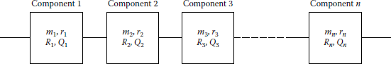
and since the n components are independent,

$\begin{array}{cccc}{R}_{\mathrm{sys}}\hfill & =\hfill & P\left(E_1\right)P\left(E_2\right)P\left(E_3\right)...P\left(E_n\right)\hfill & \left(11.62\right)\hfill \end{array}$

or

$\begin{array}{ccc}{R}_{\mathrm{sys}}\hfill & =\hfill & R_1\times R_2\times R_3\times ...R_n\hfill \end{array}$

or

$\begin{array}{cccc}{R}_{\text{sys}}\hfill & =\hfill & {\displaystyle \prod _{i=1}^n{R}_i}\hfill & \left(11.63\right)\hfill \end{array}$

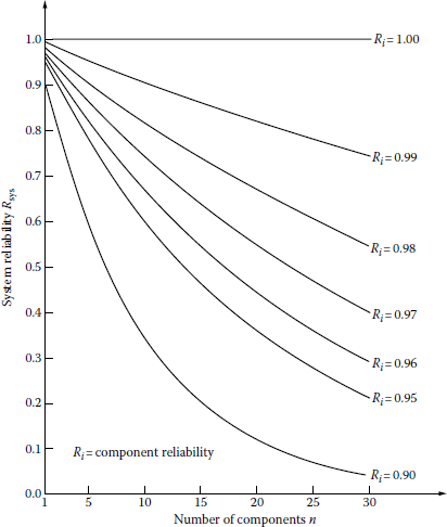
Note that Equation 11.63 is known as the product rule or the chain rule of reliability. System reliability will always be less than or equal to the least-reliable component, that is,

$\begin{array}{cccc}{R}_{\underset{i}{\text{sys}}}\hfill & \le \hfill & \min \left\{R_i\right\}\hfill & \left(11.64\right)\hfill \end{array}$

Therefore, the system reliability, due to the characteristic of the series system, is the function of the number of series components and the component reliability level. Thus, the reliability of a series system can be improved by (1) decreasing the number of series components or (2) increasing the component reliabilities. This concept has been illustrated in Figure 11.11.

Assume that the probability that a component will fail is q and it is the same for all components for a given series system. Therefore, the system reliability can be expressed as

$\begin{array}{cccc}{R}_{\text{sys}}\hfill & =\hfill & {\left(1-q\right)}^n\hfill & \left(11.65\right)\hfill \end{array}$

or, according to the binomial theorem,

$\begin{array}{cccc}{R}_{\text{sys}}\hfill & =\hfill & 1+n{\left(-q\right)}^1+\frac{n\left(n-1\right)}{2}{\left(-q\right)}^2+...+{\left(-q\right)}^n\hfill & \left(11.66\right)\hfill \end{array}$

If the probability of the component failure q is small, an approximate form for the system reliability, from Equation 11.66, can be expressed as

$\begin{array}{cccc}{R}_{\text{sys}}\hfill & \cong \hfill & 1-nq\hfill & \left(11.67\right)\hfill \end{array}$

where

n is the total number of components connected in series in the system

q is the probability of component failure

If the probabilities of component failures, that is, qi’s, are different for each component, then the approximate form of the system reliability can be expressed as

$\begin{array}{cccc}{R}_{\text{sys}}\hfill & \cong \hfill & 1-{\displaystyle \sum _{i-1}^n{q}_i}\hfill & \left(11.68\right)\hfill \end{array}$

Example 11.1

Assume that 15 identical components are going to be connected in series in a given system. If the minimum acceptable system reliability is 0.99, determine the approximate value of the component reliability.

Solution

From Equation 11.67,

$\begin{array}{ccc}{R}_{\text{sys}}\hfill & \cong \hfill & 1-nq\hfill \\ 0.99\hfill & =\hfill & 1-5\left(q\right)\hfill \end{array}$

and

$\begin{array}{ccc}q\hfill & =\hfill & 0.0007\hfill \end{array}$

Therefore, the approximate value of the component reliability required to meet the particular system reliability can be found as

$\begin{array}{ccc}{R}_i\hfill & \cong \hfill & 0.9993\hfill \end{array}$

11.5.2 Repairable Components in Series*

Consider a series system with two components, as shown in Figure 11.9. Assume that the components are independent and repairable. Therefore, the availability or the steady-state probability of success (i.e., operation) of the system can be expressed as

$\begin{array}{cccc}{A}_{\text{sys}}\hfill & =\hfill & A_1\times A_2\hfill & \left(11.69\right)\hfill \end{array}$

where

Asys is the availability of system

A1 is the availability of component 1

A2 is the availability of component 2

Since

$\begin{array}{cccc}{A}_1\hfill & =\hfill & \frac{{\overline{m}}_1}{{\overline{m}}_1+\overline{r_1}}\hfill & \left(11.70\right)\hfill \end{array}$

and

$\begin{array}{cccc}{A}_2\hfill & =\hfill & \frac{{\overline{m}}_2}{{\overline{m}}_2+\overline{r_2}}\hfill & \left(11.71\right)\hfill \end{array}$

substituting Equations 11.70 and 11.71 into Equation 11.69 gives

$\begin{array}{cccc}{A}_{\text{sys}}\hfill & =\hfill & \frac{{\overline{m}}_1}{{\overline{m}}_1+\overline{r_1}}\times \frac{{\overline{m}}_2}{{\overline{m}}_2+\overline{r_2}}\hfill & \left(11.72\right)\hfill \end{array}$

or

$\begin{array}{cccc}{A}_{\text{sys}}\hfill & =\hfill & \frac{{\overline{m}}_{\text{sys}}}{{\overline{m}}_{\text{sys}}+\overline{r_{\text{sys}}}}\hfill & \left(11.73\right)\hfill \end{array}$

where

${\overline{m}}_1$ is the mean time to failure of component 1

${\overline{m}}_2$ is the mean time to failure of component 2

${\overline{m}}_{\mathrm{sys}}$ is the mean time to failure of system

${\overline{r}}_1$ is the mean time to repair of component 1

${\overline{r}}_2$ is the mean time to repair of component 2

${\overline{r}}_{\mathrm{sys}}$ is the mean time to repair of system

The average frequency of the system failure is the sum of the average frequency of component 1 failing, given that component 2 is operable, plus the average frequency of component 2 failing while component 1 is operable. Thus,

$\begin{array}{cccc}{\overline{f}}_{\text{sys}}\hfill & =\hfill & A_2\times {\overline{f}}_1+A_1\times {\overline{f}}_2\hfill & \left(11.74\right)\hfill \end{array}$

where

${\overline{f}}_{\mathrm{sys}}$ is the average frequency of system failure

$\overline{f_i}$ is the average frequency of failure of component i

Ai is the availability of component i

Since

$\begin{array}{cccc}{\overline{f}}_i\hfill & =\hfill & \frac{1}{{\overline{m}}_i+{\overline{r}}_i}\hfill & \left(11.75\right)\hfill \end{array}$

and

$\begin{array}{cccc}{A}_i\hfill & =\hfill & \frac{{\overline{m}}_i}{{\overline{m}}_i+{\overline{r}}_i}\hfill & \left(11.76\right)\hfill \end{array}$

substituting Equations 11.75 and 11.76 into Equation 11.74 gives

$\begin{array}{cccc}{\overline{f}}_{\text{sys}}\hfill & =\hfill & \frac{1}{{\overline{m}}_1+{\overline{r}}_1}\times \frac{{\overline{m}}_2}{{\overline{m}}_2+{\overline{r}}_2}+\frac{1}{{\overline{m}}_2+{\overline{r}}_2}\times \frac{{\overline{m}}_1}{{\overline{m}}_1+{\overline{r}}_1}\hfill & \left(11.77\right)\hfill \end{array}$

Note that Equation 11.73 can be expressed as

$\begin{array}{cccc}{A}_{\text{sys}}\hfill & =\hfill & {\overline{m}}_{\text{sys}}\times {\overline{f}}_{\text{sys}}\hfill & \left(11.78\right)\hfill \end{array}$

Thus, the mean time to failure for a given series system with two components can be expressed as

$\begin{array}{cccc}{\overline{m}}_{\text{sys}}\hfill & =\hfill & \frac{1}{1/{\overline{m}}_1\times 1/{\overline{m}}_2}\hfill & \left(11.79\right)\hfill \end{array}$

Hence, the mean time to failure of a given series system with n components can be expressed as

$\begin{array}{cccc}{\overline{m}}_{\text{sys}}\hfill & =\hfill & \frac{1}{1/{\overline{m}}_1\times 1/{\overline{m}}_2+...+1/{\overline{m}}_n}\hfill & \left(11.80\right)\hfill \end{array}$

Since the reciprocal of the mean time to failure is defined as the failure rate, for the two-component system,

$\begin{array}{cccc}{\lambda }_{\text{sys}}\hfill & =\hfill & {\lambda }_1+{\lambda }_2\hfill & \left(11.81\right)\hfill \end{array}$

and for the n-component system,

$\begin{array}{cccc}{\lambda }_{\text{sys}}\hfill & =\hfill & {\lambda }_1+{\lambda }_2+{\lambda }_3+...+{\lambda }_n\hfill & \left(11.82\right)\hfill \end{array}$

Similarly, it can be shown that the mean time to repair for the given two-component series system is

$\begin{array}{cccc}{\overline{r}}_{\text{sys}}\hfill & =\hfill & \frac{{\lambda }_1\overline{r_1}+{\lambda }_2\overline{r_2}+\left({\lambda }_1\overline{r_1}\right)\left({\lambda }_2\overline{r_2}\right)}{{\lambda }_{\text{sys}}}\hfill & \left(11.83\right)\hfill \end{array}$

or, approximately,*

$\begin{array}{cccc}{\overline{r}}_{\text{sys}}\hfill & =\hfill & \frac{{\lambda }_1\overline{r_1}+{\lambda }_2\overline{r_2}}{{\lambda }_{\text{sys}}}\hfill & \left(11.84\right)\hfill \end{array}$

Therefore, the mean time to repair for an n-component series system is

$\begin{array}{cccc}{\overline{r}}_{\text{sys}}\hfill & =\hfill & \frac{{\lambda }_1\overline{r_1}+{\lambda }_2\overline{r_2}+{\lambda }_3\overline{r_3}+...+{\lambda }_n\overline{r_n}}{{\lambda }_{\text{sys}}}\hfill & \left(11.85\right)\hfill \end{array}$

11.6 Parallel Systems

11.6.1 Unrepairable Components in Parallel

Figure 11.12 shows a block diagram for a system that has two components connected in parallel. Assume that the two components are independent. Therefore, to have the system fail and not be able to perform its designated function, both components must fail simultaneously. Thus, the system unreliability is

$\begin{array}{cccc}{Q}_{\text{sys}}\hfill & =\hfill & P\left[{\overline{E}}_1\cap {\overline{E}}_2\right]\hfill & \left(11.86\right)\hfill \end{array}$

and since it is assumed that the components are independent,

$\begin{array}{cccc}{Q}_{\text{sys}}\hfill & =\hfill & P\left({\overline{E}}_1\right)P\left({\overline{E}}_2\right)\hfill & \left(11.87\right)\hfill \end{array}$

or

$\begin{array}{cccc}{Q}_{\text{sys}}\hfill & =\hfill & {\displaystyle \prod _{i=1}^2\left(1-R_i\right)}\hfill & \left(11.88\right)\hfill \end{array}$

where

$\overline{E_{\mathrm{i}}}$ is the event that component i fails

$\stackrel{}{Q_{\mathrm{i}}}$ = $P(\overline{E_i})$ is the unreliability of component i

Qsys is the unreliability of system (or system unreliability index)

Then the system reliability is given by the complementary probability as

$\begin{array}{cccc}{R}_{\text{sys}}\hfill & =\hfill & 1-{\displaystyle \prod _{i=1}^2\left(1-R_i\right)}\hfill & \left(11.89\right)\hfill \end{array}$

for this two-unit redundant system.

To generalize this concept, consider a parallel system with m independent components, as shown in Figure 11.13. Therefore, the system unreliability can be expressed as

$\begin{array}{cccc}{Q}_{\text{sys}}\hfill & =\hfill & P\left[{\overline{E}}_1\cap {\overline{E}}_2\cap {\overline{E}}_3\cap ...\cap {\overline{E}}_m\right]\hfill & \left(11.90\right)\hfill \end{array}$

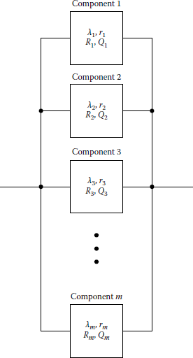
and since the m components are independent, or

$\begin{array}{cccc}{Q}_{\text{sys}}\hfill & =\hfill & P\left({\overline{E}}_1\right)P\left({\overline{E}}_2\right)P\left({\overline{E}}_3\right)...P\left({\overline{E}}_m\right)\hfill & \left(11.91\right)\hfill \end{array}$

or

$\begin{array}{cccc}{Q}_{\text{sys}}\hfill & =\hfill & Q_1\times Q_3\times Q_3\times ...\times Q_m\hfill & \left(11.92\right)\hfill \end{array}$

Therefore, the system reliability is

$\begin{array}{ccc}{R}_{\text{sys}}\hfill & =\hfill & 1-Q_{\text{sys}}\hfill \\ \hfill & =\hfill & 1-\left[Q_1\times Q_2\times Q_3\times \cdots \times Q_m\right]\hfill \\ \hfill & =\hfill & 1-\left[\left(1-R_1\right)\left(1-R_2\right)\left(1-R_3\right)\cdots \left(1-R_m\right)\right]\hfill \\ \hfill & =\hfill & 1-{\displaystyle \prod _{i=1}^m{Q}_i}\hfill \end{array}$

or

$\begin{array}{cccc}{R}_{\text{sys}}\hfill & =\hfill & 1-{\displaystyle \prod _{i=1}^m\left(1-R_i\right)}\hfill & \left(11.93\right)\hfill \end{array}$

Note that there is an implied assumption that all units are operating simultaneously and that failures do not influence the reliability of the surviving subsystems.

The instantaneous failure rate of a parallel system is a variable function of the operating time, even though the failure rates and mean times between failures of the particular components are constant. Therefore, the system reliability is the joint function of the mean time between failures of each path and the number of parallel paths. As can be seen in Figure 11.14, for a given component reliability, the marginal gain in the system reliability due to the addition of parallel paths decreases rapidly.

Thus, the greatest gain in system reliability occurs when a second path is added to a single path. The reliability of a parallel system is not a simple exponential but a sum of exponentials. Therefore, the system reliability for a two-component parallel system is

$\begin{array}{cccc}{R}_{\text{sys}}\left(t\right)\hfill & =\hfill & 1-\left(1-e^{-{\lambda }_{1}t}\right)\left(1-e^{-{\lambda }_{2}t}\right)\hfill & \hfill \\ \hfill & =\hfill & e^{-{\lambda }_{1}t}+e^{-{\lambda }_{2}t}-e^{-\left({\lambda }_1+{\lambda }_2\right)t}\hfill & \left(11.94\right)\hfill \end{array}$

where

λ1 is the failure rate of component 1

λ2 is the failure rate of component 2

11.6.2 Repairable Components in Parallel*

Consider a parallel system with two components as shown in Figure 11.12. Assume that the components are independent and repairable. Therefore, the unavailability or the steady-state probability of failure of the system can be expressed as

$\begin{array}{cccc}{U}_{\text{sys}}\hfill & =\hfill & U_1\times U_2\hfill & \left(11.95\right)\hfill \end{array}$

where

Usys is the unavailability of system

U1 is the unavailability of component 1

U2 is the unavailability of component 2

Since

$\begin{array}{cccc}{U}_1\hfill & =\hfill & 1-A_1\hfill & \hfill \\ \hfill & =\hfill & \frac{{\lambda }_1{\overline{r}}_1}{1+{\lambda }_1{\overline{r}}_1}\hfill & \left(11.96\right)\hfill \end{array}$

and

$\begin{array}{cccc}{U}_2\hfill & =\hfill & 1-A_2\hfill & \hfill \\ \hfill & =\hfill & \frac{{\lambda }_2{\overline{r}}_2}{1+{\lambda }_2{\overline{r}}_2}\hfill & \left(11.97\right)\hfill \end{array}$

substituting Equations 11.96 and 11.97 into Equation 11.95 gives

$\begin{array}{cccc}{U}_{\text{sys}}\hfill & =\hfill & \frac{{\lambda }_1{\overline{r}}_1}{1+{\lambda }_1{\overline{r}}_1}\times \frac{{\lambda }_2{\overline{r}}_2}{1+{\lambda }_2{\overline{r}}_2}\hfill & \left(11.98\right)\hfill \end{array}$

However, the average frequency of the system failure is

$\begin{array}{cccc}{\overline{f}}_{\text{sys}}\hfill & =\hfill & U_2\overline{f_1}+U_1\overline{f_2}\hfill & \left(11.99\right)\hfill \end{array}$

where

${\overline{f}}_{\mathrm{sys}}$ is the average frequency of system failure

${\overline{f}}_{\mathrm{i}}$ is the average frequency of failure of component i

Ui is the unavailability of component i

Since

$\begin{array}{cccc}{\overline{f}}_1\hfill & =\hfill & \frac{{\lambda }_1}{1+{\lambda }_1{\overline{r}}_1}\hfill & \left(11.100\right)\hfill \end{array}$

and

$\begin{array}{cccc}{\overline{f}}_2\hfill & =\hfill & \frac{{\lambda }_2}{1+{\lambda }_2{\overline{r}}_2}\hfill & \left(11.101\right)\hfill \end{array}$

substituting equation sets (11.96), (11.97) and (11.100), (11.101) into Equation 11.99 and simplifying gives

$\begin{array}{cccc}{\overline{f}}_{\text{sys}}\hfill & =\hfill & \frac{{\lambda }_1{\lambda }_2\left({\overline{r}}_1+{\overline{r}}_2\right)}{\left(1+{\lambda }_1{\overline{r}}_1\right)\left(1+{\lambda }_2{\overline{r}}_2\right)}\hfill & \left(11.102\right)\hfill \end{array}$

From Equation 11.50, the system unavailability can be expressed as

$\begin{array}{cccc}{U}_{\text{sys}}\hfill & \triangleq \hfill & \frac{{\overline{r}}_{\text{sys}}}{{\overline{T}}_{\text{sys}}}\hfill & \left(11.103\right)\hfill \end{array}$

or

$\begin{array}{cccc}{U}_{\text{sys}}\hfill & =\hfill & {\overline{r}}_{\text{sys}}\times {\overline{f}}_{\text{sys}}\hfill & \left(11.104\right)\hfill \end{array}$

so that

$\begin{array}{cccc}{\overline{r}}_{\text{sys}}\hfill & =\hfill & \frac{{\text{U}}_{\text{sys}}}{{\overline{f}}_{\text{sys}}}\hfill & \left(11.105\right)\hfill \end{array}$

Therefore, substituting Equations 11.98 and 11.102 into Equation 11.105, the average repair time (or downtime) of the two-component parallel system can be expressed as*

$\begin{array}{cccc}{\overline{r}}_{\text{sys}}\hfill & =\hfill & \frac{{\overline{r}}_1\times {\overline{r}}_2}{{\overline{r}}_1+{\overline{r}}_2}\hfill & \left(11.106\right)\hfill \end{array}$

or

$\begin{array}{cccc}\frac{1}{{\overline{r}}_{\text{sys}}}\hfill & =\hfill & \frac{1}{{\overline{r}}_1}+\frac{1}{{\overline{r}}_2}\hfill & \left(11.107\right)\hfill \end{array}$

Similarly, from Equation 11.51, the system unavailability can be expressed as

$\begin{array}{cccc}{U}_{\text{sys}}\hfill & \triangleq \hfill & \frac{{\overline{r}}_{\text{sys}}}{{\overline{r}}_{\text{sys}}+{\overline{m}}_{\text{sys}}}\hfill & \left(11.108\right)\hfill \end{array}$

from which

$\begin{array}{cccc}{\overline{m}}_{\text{sys}}\hfill & =\hfill & \frac{{\overline{r}}_{\text{sys}}\left(1-U_{\text{sys}}\right)}{U_{\text{sys}}}\hfill & \left(11.109\right)\hfill \end{array}$

Substituting Equations 11.98 and 11.106 into Equation 11.109, the average time to failure (or operation time, or uptime) of the parallel system can be expressed as

$\begin{array}{cccc}{\overline{m}}_{\text{sys}}\hfill & =\hfill & \frac{1+{\lambda }_1{\overline{r}}_1+{\lambda }_2{\overline{r}}_2}{{\lambda }_1{\lambda }_2\left({\overline{r}}_1+{\overline{r}}_2\right)}\hfill & \left(11.110\right)\hfill \end{array}$

The failure rate of the parallel system is

$\begin{array}{cccc}{\overline{\lambda }}_{\text{sys}}\hfill & \triangleq \hfill & \frac{1}{{\overline{m}}_{\text{sys}}}\hfill & \left(11.111\right)\hfill \end{array}$

or

$\begin{array}{cccc}{\lambda }_{\text{sys}}\hfill & =\hfill & \frac{{\lambda }_1{\lambda }_2\left({\overline{r}}_1+{\overline{r}}_2\right)}{1+{\lambda }_1{\overline{r}}_1+{\lambda }_2{\overline{r}}_2}\hfill & \left(11.112\right)\hfill \end{array}$

When more than two identical units are in parallel and/or when the system is not purely redundant, that is, parallel, the probabilities of the states or modes of the system can be calculated by using the binomial distribution or conditional probabilities.

Example 11.2

Figure 11.15 shows a 4 mi long distribution express feeder that is used to provide electric energy to a load center located in the downtown area of Ghost City from the Ghost River Substation. Approximately 1 mi of the feeder has been built underground due to aesthetic considerations in the vicinity of the downtown area, while the rest of the feeder is overhead. The underground feeder has two termination points. On the average, two faults per circuit-mile for the overhead section and one fault per circuit-mile for the underground section of the feeder have been recorded in the last 10 years.

The annual cable termination fault rate is given as 0.3% per cable termination. Furthermore, based on past experience, it is known that, on the average, the repair times for the overhead section, underground section, and each cable termination are 3, 28, and 3 h, respectively. Using the given information, determine the following:

1. Total annual fault rate of the feeder
2. Average annual fault restoration time of the feeder in hours
3. Unavailability of the feeder
4. Availability of the feeder

Solution

1. Total annual fault rate of the feeder is

   ${\lambda }_{\text{FDR}}={\displaystyle \sum _{i=1}^3{\lambda }_i}={\lambda }_{\text{OH}}+{\lambda }_{\text{UG}}+2{\lambda }_{\text{CT}}$

   where

   λOH is the total annual fault rate of overhead section of feeder

   λUG is the total annual fault rate of underground section of feeder

   λCT is the total annual fault rate of cable terminations

   Therefore,

   $\begin{array}{ccc}{\lambda }_{\text{FDR}}\hfill & =\hfill & 3\left(\frac{2}{10}\right)+1\left(\frac{1}{10}\right)+2\left(0.003\right)\hfill \\ \hfill & =\hfill & 0.706\text{faults/year}\hfill \end{array}$

2. Average fault restoration time of the feeder per fault is

   ${\overline{r}}_{\text{FDR}}={\displaystyle \sum _{i=1}^3{\overline{r}}_i}={\overline{r}}_{\text{OH}}+{\overline{r}}_{\text{UG}}+2{\overline{r}}_{\text{CT}}$

   where

   ${\overline{r}}_{\mathrm{OH}}$ is the average repair time for overhead section of feeder, h

   ${\overline{r}}_{\mathrm{UG}}$ is the average repair time for underground section of feeder, h

   ${\overline{r}}_{\mathrm{CT}}$ is the average repair time per cable termination, h

   Thus,

   $\begin{array}{ccc}{\overline{r}}_{\text{FDR}}\hfill & =\hfill & 3+28+2\left(3\right)\hfill \\ \hfill & =\hfill & 37\text{h}\hfill \end{array}$

   However, the average annual fault restoration time of the feeder is

   $\begin{array}{ccc}{r}_{\text{FDR}}\hfill & =\hfill & \frac{{\sum }_{i=1}^3{\lambda }_i\times r_i}{{\sum }_{i=1}^3{\lambda }_i}\hfill \end{array}$

   or

   $\begin{array}{ccc}{\overline{r}}_{\text{FDR}}\hfill & =\hfill & \frac{\left(I_{\text{OH}}\times {\lambda }_{\text{OH}}\right)\left({\overline{r}}_{\text{OH}}\right)\left(I_{\text{UG}}\times {\lambda }_{\text{UG}}\right)\left({\overline{r}}_{\text{UG}}\right)+\left(2{\lambda }_{\text{CT}}\right)\left({\overline{r}}_{\text{CT}}\right)}{{\lambda }_{\text{FDR}}}\hfill \\ \hfill & =\hfill & \frac{\left(3\times 0.2\right)\left(3\right)+\left(1\times 0.1\right)\left(28\right)+\left(2\times 0.003\right)\left(3\right)}{0.706}\hfill \\ \hfill & =\hfill & \frac{4.618}{0.706}\hfill \\ \hfill & =\hfill & 6.54\mathrm{h}\hfill \end{array}$

3. Unavailability of the feeder is

   $\begin{array}{ccc}{U}_{\text{FDR}}\hfill & =\hfill & \frac{{\overline{r}}_{\text{FDR}}}{{\overline{r}}_{\text{FDR}}+{\overline{m}}_{\text{FDR}}}\hfill \end{array}$

   where

   $\begin{array}{ccc}{\overline{m}}_{\text{FDR}}\hfill & =\hfill & \text{annual mean time to failure}\hfill \\ \hfill & =\hfill & 8760-{\overline{r}}_{\text{FDR}}\hfill \\ \hfill & =\hfill & 8760-6.54\hfill \\ \hfill & =\hfill & 8753.46\text{h/year}\hfill \end{array}$

   Therefore,

   $\begin{array}{ccc}{U}_{\text{FDR}}\hfill & =\hfill & \frac{6.54}{6.54+8753.46}\hfill \\ \hfill & =\hfill & \mathrm{0.0007\%}\text{or}0.07\%\hfill \end{array}$

4. Availability of the feeder is

   $\begin{array}{ccc}{\lambda }_{\text{FDR}}\hfill & =\hfill & 1-U_{\text{FDR}}\hfill \\ \hfill & =\hfill & 1-0.007\hfill \\ \hfill & =\hfill & 0.9993\text{or}99.93\%\hfill \end{array}$

Example 11.3

Assume that the primary main feeder shown in Figure 11.16 is manually sectionalized and that presently only the first three feeder sections exist and serve customers A, B, and C. The annual average fault rates for primary main and laterals are 0.08 and 0.2 fault/circuit-mile, respectively. The average repair times for each primary main section and for each primary lateral are 3.5 and 1.5 h, respectively. The average time for manual sectionalizing of each feeder section is 0.75 h. Assume that at the time of having one of the feeder sections in fault, the other feeder section(s) are sectionalized manually as long as they are not in the mainstream of the fault current, that is, not in between the faulted section and the circuit breaker. Otherwise, they have to be repaired also.

Based on the given information, prepare an interruption analysis study for the first contingency only, that is, ignore the possibility of simultaneous outages, and determine the following:

1. The total annual sustained interruption rates for customers A, B, and C.
2. The average annual repair times, that is, downtimes, for customers A, B, and C.
3. Write the necessary codes to solve the problem in MATLAB.

Solution

1. Total annual sustained interruption rates for customers A, B, and C are

   $\begin{array}{ccc}{\lambda }_{\text{A}}\hfill & =\hfill & {\displaystyle \sum _{i=1}^4{\lambda }_i={\lambda }_{\sec .1}+{\lambda }_{\sec .2}+{\lambda }_{\sec .3}+{\lambda }_{\text{lat}.A}}\hfill \\ \hfill & =\hfill & \text{(1mi)(0}\text{.08)+(1mi)(0}\text{.08)+(1mi)(0}\text{.08)}+\text{(2mi)(0}\text{.02)}\hfill \\ \hfill & =\hfill & 0.64\text{fault/year}\hfill \end{array}$

   $\begin{array}{ccc}{\lambda }_B\hfill & =\hfill & {\displaystyle \sum _{i=1}^4{\lambda }_i={\lambda }_{\sec .1}+{\lambda }_{\sec .2}+{\lambda }_{\sec .3}+{\lambda }_{\text{lat}.B}}\hfill \\ \hfill & =\hfill & \text{(1mi)(0}\text{.08)+(1mi)(0}\text{.08)+(1mi)(0}\text{.08)}+\text{(1.5mi)(0}\text{.02)}\hfill \\ \hfill & =\hfill & 0.54\text{fault/year}\hfill \end{array}$

   ${\lambda }_C={\lambda }_B=0.54\text{fault/year}$

2. Average annual repair time, that is, downtime (or restoration time), for customer A is

   ${\overline{r}}_A=\frac{{\lambda }_{\sec .1}\times {\overline{r}}_{\text{fault}}+{\lambda }_{\sec .2}\times {\overline{r}}_{\text{MS}}+{\lambda }_{\sec .3}\times {\overline{r}}_{\text{MS}}+{\lambda }_{\text{lat.}A}\times {\overline{r}}_{\text{lat fault}}}{{\lambda }_A}$

   where

   ${\overline{r}}_A$ average repair time for customer A

   $\stackrel{}{{\lambda }_{sec\text{.}i}}$ is the total fault rate for feeder section i per year

   ${\overline{r}}_{\mathrm{fault}}$ is the average repair time for faulted primary main section

   ${\overline{r}}_{\text{lat.fault}}$ is the average repair time for faulted primary lateral

   ${\overline{r}}_{\text{MS}}$ is the average time for manual sectionalizing per section

   λlat. A is the total fault rate for lateral A per year

   Therefore,

   $\begin{array}{ccc}{\overline{r}}_A\hfill & =\hfill & \frac{\left(0.08\right)\left(3.5+0.08\right)\left(0.75\right)+\left(0.08\right)\left(0.75\right)+\left(2\times 0.2\right)\left(1.5\right)1.00}{0.64}\hfill \\ \hfill & =\hfill & \frac{1.00}{0.64}\hfill \\ \hfill & =\hfill & 1.56\text{h}\hfill \end{array}$

   Similarly, for customer B,

   $\begin{array}{ccc}{\overline{r}}_B\hfill & =\hfill & \frac{{\lambda }_{\sec .1}\times {\overline{r}}_{\text{fault}}+{\lambda }_{\sec .2}\times {\overline{r}}_{\text{MS}}+{\lambda }_{\sec .3}\times {\overline{r}}_{\text{MS}}+{\lambda }_{\text{lat}.B}\times {\overline{r}}_{\text{lat,fault}}}{{\lambda }_B}\hfill \\ \hfill & =\hfill & \frac{\left(0.08\right)\left(3.5\right)+\left(0.08\right)\left(3.5\right)+\left(0.08\right)\left(0.75\right)+\left(1.5\times 0.2\right)\left(1.5\right)}{0.54}\hfill \\ \hfill & =\hfill & \frac{1.07}{0.54}\hfill \\ \hfill & =\hfill & 1\text{.98h}\hfill \end{array}$

   and for customer C,

   $\begin{array}{ccc}{\overline{r}}_C\hfill & =\hfill & \frac{{\lambda }_{\sec .1}\times {\overline{r}}_{\text{fault}}+{\lambda }_{\sec .2}\times {\overline{r}}_{\text{MS}}+{\lambda }_{\sec .3}\times {\overline{r}}_{\text{MS}}+{\lambda }_{\text{lat}.C}\times {\overline{r}}_{\text{lat,fault}}}{{\lambda }_B}\hfill \\ \hfill & =\hfill & \frac{\left(0.08\right)\left(3.5\right)+\left(0.08\right)\left(3.5\right)+\left(0.08\right)\left(3.5\right)+\left(1.5\times 0.2\right)\left(1.5\right)}{0.54}\hfill \\ \hfill & =\hfill & \frac{1.29}{0.54}\hfill \\ \hfill & =\hfill & 2\text{.39h}\hfill \end{array}$

3. Here is the MATLAB script:

   clc

   clear

   % System parameters

   % failure rates

   lambda_sec1 = 1*0.08;

   lambda_sec2 = lambda_sec1;

   lambda_sec3 = lambda_sec1;

   lambda_sec4 = lambda_sec1;

   lambda_latA = 2*0.2;

   lambda_latB = 1.5*0.2;

   lambda_latC = 1.5*0.2;

   lambda_latD = 1*0.2;

   lambda_latE = 1.5*0.2;

   lambda_latF = 2*0.2;

   % repair times

   r_sec = 3.5;

   r_lat = 1.5;

   r_MS = 0.75;% manual sectionalizing

   % Solution to part a

   % Total annual sustained interruption rates for customers A, B and C

   lambdaA = lambda_sec1 + lambda_sec2 + lambda_sec3 + lambda_latA

   lambdaB = lambda_sec1 + lambda_sec2 + lambda_sec3 + lambda_latB

   lambdaC = lambdaB

   % Solution to part b

   % Average annual repair time for customers A, B and C

   rA = (lambda_sec1*r_sec + lambda_sec2*r_MS + lambda_sec3*r_MS + lambda_latA*r_lat)/lambdaA

   rB = (lambda_sec1*r_sec + lambda_sec2*r_sec + lambda_sec3*r_MS + lambda_latB*r_lat)/lambdaB

   rC = (lambda_sec1*r_sec + lambda_sec2*r_sec + lambda_sec3*r_sec + lambda_latC*r_lat)/lambda