
7.4 Percent Power (or Copper) Loss
The percent power (or conductor) loss of a circuit can be expressed as
%I2R=PLSPr×100=I2RPr×100(7.59)
where
PLS is the power loss of a circuit, kW
= I2R
Pr is the power delivered by the circuit, kW
The conductor I2R losses at a load factor of 0.6 can readily be found from Table 7.5 for various voltage levels.
Conductor I2R Losses, kWh/(mi year), at 7.2/12.5 kV and a Load Factor of 0.6
Single Phase |
“V” Phase |
Three Phase |
||||||||||||
|---|---|---|---|---|---|---|---|---|---|---|---|---|---|---|
Annual Peak |
6 |
4 |
2 |
6 |
4 |
2 |
6 |
4 |
2 |
1 |
1/0 |
2/0 |
||
Load (kW) |
8 Copper |
4 ACSR |
2 ACSR |
1/0 |
8 |
4 ACSR |
2 ACSR |
1/0 |
4 ACSR |
2 ACSR |
1/0 |
2/0 |
3/0 |
4/0 |
20 |
124 |
82 |
55 |
37 |
62 |
41 |
27 |
19 |
25 |
16 |
10 |
|||
40 |
495 |
329 |
218 |
149 |
248 |
164 |
109 |
75 |
99 |
63 |
39 |
31 |
||
60 |
1,110 |
740 |
491 |
335 |
557 |
370 |
246 |
168 |
224 |
141 |
88 |
70 |
56 |
|
80 |
1,980 |
1,320 |
873 |
596 |
990 |
658 |
437 |
298 |
398 |
250 |
157 |
125 |
99 |
78 |
100 |
3,100 |
2,060 |
1,360 |
932 |
1,550 |
1,030 |
682 |
466 |
621 |
391 |
245 |
195 |
154 |
122 |
120 |
4,460 |
2,960 |
1,960 |
1,340 |
2,230 |
1,480 |
982 |
671 |
895 |
563 |
353 |
280 |
222 |
176 |
140 |
6,070 |
4,030 |
2,670 |
1,830 |
3,030 |
2,010 |
1,340 |
913 |
1,220 |
766 |
481 |
382 |
302 |
240 |
160 |
7,920 |
5,260 |
3,490 |
2,390 |
3,960 |
2,630 |
1,750 |
1,190 |
1,590 |
1,000 |
628 |
498 |
395 |
313 |
180 |
10,000 |
6,660 |
4,420 |
3,020 |
5,010 |
3,330 |
2,210 |
1,510 |
2,010 |
1,270 |
795 |
631 |
500 |
396 |
200 |
12,400 |
8,220 |
5,460 |
3,730 |
6,190 |
4,110 |
2,730 |
1,860 |
2,490 |
1,560 |
982 |
779 |
617 |
489 |
225 |
15,700 |
10,400 |
6,910 |
4,720 |
7,830 |
5,200 |
3,450 |
2,360 |
3,150 |
1,980 |
1240 |
986 |
780 |
619 |
250 |
19,300 |
12,800 |
8,530 |
5,820 |
9,670 |
6,420 |
4,260 |
2,910 |
3,880 |
2,440 |
1530 |
1220 |
964 |
764 |
275 |
23,400 |
15,500 |
10,300 |
7,050 |
11,700 |
7,770 |
5,160 |
3,520 |
4,700 |
2,960 |
1860 |
1470 |
1170 |
925 |
300 |
18,500 |
12,300 |
8,390 |
13,900 |
9,250 |
6,140 |
4,190 |
5,590 |
3,520 |
2210 |
1750 |
1390 |
1100 |
|
325 |
21,700 |
14,400 |
9,840 |
16,300 |
10,900 |
7,210 |
4,920 |
6,560 |
4,130 |
2590 |
2060 |
1630 |
1280 |
|
350 |
16,700 |
11,400 |
18,900 |
12,600 |
8,360 |
5,710 |
7,610 |
4,790 |
3010 |
2380 |
1890 |
1500 |
||
375 |
19,200 |
13,100 |
21,800 |
14,400 |
9,590 |
6,550 |
8,740 |
5,500 |
3450 |
2740 |
2170 |
1720 |
||
400 |
21,800 |
14,900 |
24,800 |
16,400 |
10,900 |
7,450 |
9,940 |
6,260 |
3930 |
3120 |
2470 |
1960 |
||
450 |
18,900 |
20,800 |
13,800 |
9,430 |
12,600 |
7,920 |
4970 |
3940 |
3120 |
2480 |
||||
500 |
23,300 |
25,700 |
17,100 |
11,600 |
15,500 |
9,780 |
6140 |
4870 |
3850 |
3060 |
||||
550 |
20,600 |
14,100 |
18,800 |
11,800 |
7420 |
5890 |
4660 |
3700 |
||||||
600 |
24,600 |
16,800 |
22,400 |
14,100 |
8840 |
7010 |
5550 |
4400 |
||||||
Source: Rural Electrification Administration, U.S. Department of Agriculture: Economic Design of Primary Lines for Rural Distribution Systems, REA Bulletin, 60, 1960.
Note: This table is calculated for a PF of 90%. To adjust for a different PF, multiply these values by the factor of k = (90)2/(PF)2.
For 7.62/13.2 kV, multiply these values by 0.893; for 14.4/24.9 kV, multiply by 0.25.
At times, in ac circuits, the ratio of percent power, or conductor, loss to percent voltage regulation can be used, and it is given by the following approximate expression:
%I2R%VD=cosϕcosθ×cos(ϕ−θ)(7.60)
where
% I2R is the percent power loss of a circuit
% VD is the percent voltage drop of the circuit
ϕ is the impedance angle = tan–1 (X/R)
θ is the power-factor angle
7.5 Method to Analyze Distribution Costs
To make any meaningful feeder-size selection, the distribution engineer should make a cost study associated with feeders in addition to the voltage-drop and power-loss considerations. The cost analysis for each feeder size should include (1) investment cost of the installed feeder, (2) cost of energy lost due to I2R losses in the feeder conductors, and (3) cost of demand lost, that is, the cost of useful system capacity lost (including generation, transmission, and distribution systems), in order to maintain adequate system capacity to supply the I2R losses in the distribution feeder conductors. Therefore, the total annual feeder cost of a given size feeder can be expressed as
TAC = AIC+AEC+ADC $/mi(7.61)
where
TAC is the total annual equivalent cost of feeder, $/mi
AIC is the annual equivalent of investment cost of installed feeder, $/mi
AEC is the annual equivalent of energy cost due to I2R losses in feeder conductors, $/mi
ADC is the annual equivalent of demand cost incurred to maintain adequate system capacity to supply I2R losses in feeder conductors, $/mi
7.5.1 Annual Equivalent of Investment Cost
The annual equivalent of investment cost of a given size feeder can be expressed as
AIC = ICF×iF$/mi(7.62)
where
AIC is the annual equivalent of investment cost of a given size feeder, $/mi
ICF is the cost of installed feeder, $/mi
iF is the annual fixed charge rate applicable to feeder
The general utility practice is to include cost of capital, depreciation, taxes, insurance, and operation and maintenance (O&M) expenses in the annual fixed charge rate or so-called carrying charge rate. It is given as a decimal.
7.5.2 Annual Equivalent of Energy Cost
The annual equivalent of energy cost due to I2R losses in feeder conductors can be expressed as
AEC=3I2R×EC×FLL×FLSA×8760$/mi(7.63)
where
AEC is the annual equivalent of energy cost due to I2R losses in feeder conductors, $/mi
EC is the cost of energy, $/kWh
FLL is the load-location factor
FLS is the loss factor
FLSA is the loss-allowance factor
The load-location factor of a feeder with uniformly distributed load can be defined as
FLL=sl(7.64)
where
FLL is the load-location factor in decimal
s is the distance of point on feeder where total feeder load can be assumed to be concentrated for the purpose of calculating I2R losses
ℓ is the total feeder length, mi
The loss factor can be defined as the ratio of the average annual power loss to the peak annual power loss and can be found approximately for urban areas from
FLS=0.3FLD+0.7F2LD(7.65)
and for rural areas [6],
FLS=0.16FLD+0.84F2LD
The loss-allowance factor is an allocation factor that allows for the additional losses incurred in the total power system due to the transmission of power from the generating plant to the distribution substation.
7.5.3 Annual Equivalent of Demand Cost
The annual equivalent of demand cost incurred to maintain adequate system capacity to supply the I2R losses in the feeder conductors can be expressed as
ADC=3I2R×FLL×FPR×FR ×FLSA[(CG×iG)+(CT×iT)+(CS×iS)]$/mi(7.66)
where
ADC is the annual equivalent of demand cost incurred to maintain adequate system capacity to supply 12R losses in feeder conductors, $/mi
FLL is the load-location factor
FPR is the peak-responsibility factor
FR is the reserve factor
FLSA is the loss-allowance factor
CG is the cost of (peaking) generation system $/kVA
CT is the cost of transmission system, $/kVA
CS is the cost of distribution substation, $/kVA
iG is the annual fixed charge rate applicable to generation system
iT is the annual fixed charge rate applicable to transmission system
iS is the annual fixed charge rate applicable to distribution substation
The reserve factor is the ratio of total generation capability to the total load and losses to be supplied. The peak-responsibility factor is a per unit value of the peak feeder losses that are coincident with the system peak demand.
7.5.4 Levelized Annual Cost
In general, the costs of energy and demand and even O&M expenses vary from year to year during a given time, as shown in Figure 7.16a; therefore, it becomes necessary to levelize these costs over the expected economic life of the feeder, as shown in Figure 7.16b.
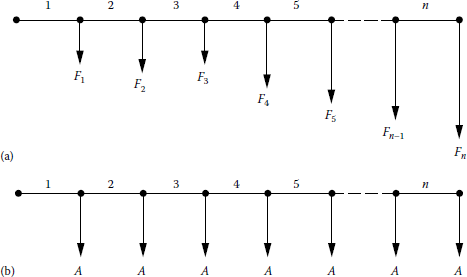
Illustration of the levelized annual cost concept: (a) unlevelized annual cost flow diagram and (b) levelized cost flow diagram.
Assume that the costs occur discretely at the end of each year, as shown in Figure 7.16a. The levelized annual cost* of equal amounts can be calculated as
A=[F1(PF)i1+F2(PF)i2+F3(PF)i3+...+Fn(PF)in](AP)in(7.67)
or
A=[n∑j=1Fi(PF)ij](AP)in(7.68)
where
A is the levelized annual cost, $/year
Fi is the unequal (or actual or unlevelized) annual cost, $/year
n is the economic life, year
i is the interest rate
(P/F)in is the present worth (or present equivalent) of a future sum factor (with i interest rate and n years of economic life), also known as single-payment discount factor
(A/P)in is the uniform series worth of a present sum factor, also known as capital-recovery factor
The single-payment discount factor and the capital-recovery factor can be found from the compounded-interest tables or from the following equations, respectively,
(PF)in=1(1+i)n(7.69)
and
(AP)in=i(1+i)n(1+i)n−1(7.70)
Example 7.15
Assume that the following data have been gathered for the system of the NL&NP Company.
- Feeder length = 1 mi
- Cost of energy = 20 mills/kWh (or $0.02/kWh)
- Cost of generation system = $200/kW
- Cost of transmission system = $65/kW
- Cost of distribution substation = $20/kW
- Annual fixed charge rate for generation = 0.21
- Annual fixed charge rate for transmission = 0.18
- Annual fixed charge rate for substation = 0.18
- Annual fixed charge rate for feeders = 0.25
- Interest rate = 12%
- Load factor = 0.4
- Loss-allowance factor = 1.03
- Reserve factor = 1.15
- Peak-responsibility factor = 0.82
Table 7.6 gives cost data for typical ACSR conductors used in rural areas at 12.5 and 24.9 kV. Table 7.7 gives cost data for typical ACSR conductors used in urban areas at 12.5 and 34.5 kV. Using the given data, develop nomographs that can be readily used to calculate the total annual equivalent cost of the feeder in dollars per mile.
Typical ACSR Conductors Used in Rural Areas
Conductor Ground Wire |
Conductor Ground Wire |
Installation |
Total |
|||
|---|---|---|---|---|---|---|
Cost and Hardware Installed |
||||||
Size |
Size |
Weight (lb) |
Weight (lb) |
$/lb |
Cost ($) |
Feeder Cost ($) |
At 12.5 kV |
||||||
#4 |
#4 |
356 |
356 |
0.6 |
6,945.6 |
7,800 |
1/0 |
#2 |
769 |
566 |
0.6 |
7,176.2 |
8,900 |
3/0 |
1/0 |
1223 |
769 |
0.6 |
7,737.2 |
10,400 |
4/0 |
1/0 |
1542 |
769 |
0.6 |
8,563 |
11,800 |
266.8 kcmil |
1/0 |
1802 |
769 |
0.6 |
9,985 |
13,690 |
477 kcmil |
1/0 |
3642 |
769 |
0.6 |
10,967 |
17,660 |
At 24.9 kV |
||||||
#4 |
#4 |
356 |
356 |
0.6 |
7,605.6 |
8,460 |
1/0 |
#2 |
769 |
566 |
0.6 |
7,856.2 |
9,580 |
3/0 |
1/0 |
1223 |
769 |
0.6 |
8,217.2 |
10,880 |
4/0 |
1/0 |
1542 |
769 |
0.6 |
8,293 |
11,530 |
266.8 kcmil |
1/0 |
1802 |
769 |
0.6 |
9,615 |
13,320 |
477 kcmil |
1/0 |
3462 |
769 |
0.6 |
11,547 |
18,240 |
Typical ACSR Conductors Used in Urban Areas
Conductor Ground Wire |
Conductor Ground Wire |
Cost |
Installation and Hardware Installed |
Total |
||
|---|---|---|---|---|---|---|
Size |
Size |
Weight (lb) |
Weight (lb) |
$/lb |
Cost ($) |
Feeder Cost ($) |
At 12.5 kV |
||||||
#4 |
#4 |
356 |
356 |
0.6 |
21,145.6 |
22,000 |
1/0 |
#4 |
769 |
356 |
0.6 |
22,402.2 |
24,000 |
3/0 |
#4 |
1223 |
356 |
0.6 |
24,585 |
27,000 |
477 kcmil |
1/0 |
3462 |
769 |
0.6 |
28,307 |
35,000 |
At 34.5 kV |
||||||
#4 |
#4 |
356 |
356 |
0.6 |
21,375.6 |
22,230 |
1/0 |
#4 |
769 |
356 |
0.6 |
22,632.2 |
24,230 |
3/0 |
#4 |
1223 |
356 |
0.6 |
24,815 |
27,230 |
477 kcmil |
1/0 |
3462 |
769 |
0.6 |
28,537 |
35,230 |
Solution
Using the given and additional data and appropriate equations from Section 7.5, the following nomographs have been developed. Figures 7.17 and 7.18 give nomographs to calculate the total annual equivalent cost of ACSR feeders of various sizes for rural and urban areas, respectively, in thousands of dollars per mile.

Total annual equivalent cost of ACSR feeders for rural areas in thousands of dollars per mile: (a) 477 cmil, 26 strands, (b) 266.8 cmil, 6 strands, AWG 4/0, and AWG 3/0.

Total annual equivalent cost of ACSR feeders for urban areas in thousands of dollars per mile: (a) 477 cmil, 26 strands, (b) AWG 3/0, (c) AWG 1/0, and (d) AWG 4, 7 strands.
Example 7.16
The NL&NP power and light company is required to serve a newly developed residential area. There are two possible routes for the construction of the necessary power line. Route A is 18 miles long and goes around a lake. It has been estimated that the required overhead power line will cost $8000 per mile to build and $350 per mile per year to maintain. Its salvage value will be $1500 per mile at the end of its useful life of 20 years.
On the other hand, route B is 6 miles long and is an underwater line that goes across the lake. It has been estimated that the required underwater line using submarine power cables will cost $21,000 per mile to build and $1,200 per mile per year to maintain. Its salvage value will be $6000 per mile at the end of 20 years. Assume that the fixed charge rate is 10% and that the annual ad valorem (property) taxes are 3% of the first cots of each power line. Use any engineering economy interest tables and determine the economically preferable alternative.
Solution
Route A: The first cost of the overhead power line is
P=($8,000/mile)(18miles)=$144,000
and its estimated salvage value is
F=($1,500/mile)(18 miles)=$27,000
The annual equivalent cost of capital invested in the line is
A1=$144,000(AP)10%20−$27,000(AF)10%20=$144,000(0.11746)−$27,000(0.01746)=$16,443
The annual equivalent cost of the tax and maintenance is
A2=($144,000)(3%)+($350/mile)(18miles)=$10,620
Route B: The first cost of the submarine power line is
P=($21,000/mile)(6 miles)=$126,000
and its estimated salvage value is
F=($6,000/mile)(6 miles)=$36,000
Its annual equivalent cost of capital invested is
A1=$126,000(AP)10%20−$36,000(AF)10%20=$14,171
The annual equivalent cost of the tax and maintenance is
A2=($126,000)(3%)+($1,200/mile)(6miles)=$10,980
The total annual equivalent cost of the submarine power line is
A=A1+A2=$14,171+$10,980=$25,151
Hence, the economically preferable alternative is route B. Of course, if the present worth of the costs are calculated, the conclusion would still be the same. For example, the present worth of costs for A and B are
PWA=$27,063(PA)10%20=$230,414
and
PWB=$25,151(PA)10%20=$214,136
Thus, route B is still the preferred route.
Example 7.17
Use the data given in Example 6.6 and assume that the fixed charge rate is 0.15, and zero salvage values are expected at the end of useful lives of 30 years for each alternative. But the salvage value for 9 MVA capacity line is $2000 at the end of the 10th year. Use a study period of 30 years and determine the following:
- The annual equivalent cost of 9 MVA capacity line.
- The annual equivalent cost of 15 MVA capacity line.
- The annual equivalent cost of the upgrade option if the upgrade will take place at the end of 10 years. Use an average value of $5000 at the end of 20 years for the new 15 MVA upgrade line.
Solution
- The annual equivalent cost of 9 MVA capacity line is
A1=$120,000(AP)15%30=$120,000(0.15230)=$18,276 per mile per year
- A2=$150,000(AP)15%30=$150,000(0.15230)=$22,845
- The annual equivalent cost of 15 MVA capacity line is
A2=[$120,000−$2,000(PF)15%10+$200,000(PF)15%10−$5,000(PF)15%30](AP)15%30=[$120,000−$2,000(0.2472)+$200,000(0.2472)−$5,000(0.0151)](0.15230)=$25,718.92
As it can be seen, the upgrade option is still the bad option. Furthermore, if one considers the 9 MVA vs. 15 MVA capacities, building the 15 MVA capacity line from the start is still the best option.
7.6 Economic Analysis of Equipment Losses
Today, the substantially escalating plant, equipment, energy, and capital costs make it increasingly more important to evaluate losses of electric equipment (e.g., power or distribution transformers) before making any final decision for purchasing new equipment and/or replacing (or retiring) existing ones. For example, nowadays it is not uncommon to find out that a transformer with lower losses but higher initial price tag is less expensive than the one with higher losses but lower initial price when total cost over the life of the transformer is considered.
However, in the replacement or retirement decisions, the associated cost savings in O&M costs in a given life cycle analysis* or life cycle cost study must be greater than the total purchase price of the more efficient replacement transformer. Based on the “sunk cost” concept of engineering economy, the carrying charges of the existing equipment do not affect the retirement decision, regardless of the age of the existing unit. In other words, the fixed, or carrying, charges of an existing equipment must be amortized (written off) whether the unit is retired or not.
The transformer cost study should include the following factors:
- Annual cost of copper losses
- Annual cost of core losses
- Annual cost of exciting current
- Annual cost of regulation
- Annual cost of fixed charges on the first cost of the installed equipment
These annual costs may be different from year to year during the economical lifetime of the equipment. Therefore, it may be required to levelize them, as explained in Section 7.5.4. Read Section 6.7 for further information on the cost study of the distribution transformers. For the economic replacement study of the power transformers, the following simplified technique may be sufficient. Dodds [10] summarizes the economic evaluation of the cost of losses in an old and a new transformer step by step as given in the following text:
- Determine the power ratings for the transformers as well as the peak and average system loads.
- Obtain the load and no-load losses for the transformers under rated conditions.
- Determine the original cost of the old transformer and the purchase price of the new one.
- Obtain the carrying charge rate, system capital cost rate, and energy cost rate for your particular utility.
- Calculate the transformer carrying charge and the cost of losses for each transformer. The cost of losses is equal to the system carrying charge plus the energy charge.
- Compare the total cost per year for each transformer. The total cost is equal to the sum of the transformer carrying charge and the cost of losses.
- Compare the total cost per year of the old and new transformers. If the total cost per year of the new transformer is less, replacement of the old transformer can be economically justified.
Problems
- 7.1 Consider Figure P7.1 and repeat Example 7.5.
- 7.2 Repeat Example 7.7, using a transformer with 75 kVA capacity.
- 7.3 Repeat Example 7.7, assuming four services per transformer. Here, omit the UG SL. Assume that there are six transformers per block, that is, one transformer at each pole location.
- 7.4 Repeat Problem 7.3, using a 75 kVA transformer.
- 7.5 Repeat Example 7.8, using a 100 kVA transformer and #3/0 AWG and #2 AWG cables for the SLs and SDs, respectively.
- 7.6 Repeat Example 7.10. Use the nominal primary voltage of 19,920/34,500 V and assume that the remaining data are the same.
- 7.7 Assume that a three-conductor dc overhead line with equal conductor sizes (see Figure P7.7) is considered to be employed to transmit three-phase three-conductor ac energy at 0.92 power factor.
If voltages to ground and transmission line efficiencies are the same for both direct and alternating currents, and the load is balanced, determine the change in the power transmitted in percent.
- 7.8 Assume that a single-phase feeder circuit has a total impedance of 1 + j3 Ω for lines and/or transformers. The receiving-end voltage and load current are 2400∠ 0° V and 50 ∠–30° A, respectively. Determine the following:
- The power factor of the load.
- The load power factor for which the voltage drop is maximum, using Equation 7.51.
- Repeat part (b), using Equation 7.52.
- 7.9 An unbalanced three-phase wye-connected and grounded load is connected to a balanced three-phase four-wire source. The load impedance Za, Zb, and Zc are given as 70 ∠ 30°, 85 ∠–40°, and 50 ∠35° Ω/phase, respectively, and the phase a line voltage has an effective value of 13.8 kV: Use the line-to-neutral voltage of phase a as the reference and determine the following:
- The line and neutral currents
- The total power delivered to the loads
- 7.10 Consider Figure P7.1 and assume that the impedances of the three line segments from left to right are 0.1 + j0.3, 0.1 + j0.1, and 0.08 + j0.12 Ω/phase, respectively. Also assume that this three-phase three-wire 480-V secondary system supplies balanced loads at A, B, and C. The loads at A, B, and C are represented by 50 A with a lagging power factor of 0.85, 30 A with a lagging power factor of 0.90, and 50 A with a lagging power factor of 0.95, respectively. Determine the following:
- The total voltage drop in one phase of the lateral using the approximate method
- The real power per phase for each load
- The reactive power per phase for each load
- The kilovoltampere output and load power factor of the distribution transformer
- 7.11 Assume that bulk power substation 1 supplies substations 2 and 3, as shown in Figure P7.11, through three-phase lines. Substations 2 and 3 are connected to each other over a tie line, as shown. Assume that the line-to-line voltage is 69 kV and determine the following:
- The voltage difference between substations 2 and 3 when tie line 23 is open-circuited
- The line currents when all three lines are connected as shown in the figure
- The total power loss in part (a)
- The total power loss in part (b).
- 7.12 Repeat Example 7.6, assuming 50% lagging power factor for all loads.
- 7.13 Resolve Example 7.4 by using MATLAB and assuming four services per transformer. Here, omit the UG SL. Assume that there are six transformers per block, that is, one transformer at each pole location.


References
1. Morrison, C.: A Linear approach to the problem of planning new feed points into a distribution system, AIEE Trans., 82, pt. III (PAS) December 1963, 819–832.
2. Westinghouse Electric Corporation: Electric Utility Engineering Reference Book-Distribution Systems, Vol. 3, Westinghouse Electric Corporation, East Pittsburgh, PA, 1965.
3. Fink, D. G. and H. W. Beaty: Standard Handbook for Electrical Engineers. 11th edn., McGraw-Hill, New York, 1978.
4. Gönen, T. et al.: Development of Advanced Methods for Planning Electric Energy Distribution Systems, US Department of Energy, October 1979. Available from the National Technical Information Service, US Department of Commerce, Springfield, VA.
5. Gönen, T. and D. C. Yu: A comparative analysis of distribution feeder costs, Southwest Electrical Exposition and IEEE Conference Proceedings, Houston, TX, January 22–24, 1980.
6. Rural Electrification Administration: U.S. Department of Agriculture: Economic Design of Primary Lines for Rural Distribution Systems, REA Bulletin, May, 1960, pp. 60–69.
7. Gönen, T. and D. C. Yu: A distribution system planning model, Control of Power Systems Conference Proceedings, Oklahoma City, OK, March 17–18, 1980, pp. 28–34.
8. Schlegel, M. C.: New selection method reduces conductor losses, Electr. World, February 1, 1977, 43–44.
9. Light, J.: An economic approach to distribution conductor size selection, paper presented at the Missouri Valley Electric Association 49th Annual Engineering Conference, Kansas City, MO, April 12–14, 1978.
10. Dodds, T. H.: Costs of losses can economically justify replacement of an old transformer with a new one, The Line, 80, 2, July 1980, 25–28.
11. Smith, R. W. and D. J. Ward: Does early distribution transformer retirement make sense? Electric. Forum, 6, 3, 1980, 6–9.
12. Delaney, M. B.: Economic analysis of electrical equipment losses, The Line, 74, 4, 1974, 7–8.
13. Klein, K. W.: Evaluation of distribution transformer losses and loss ratios, Elec. Light Power, July 15, 1960, 56–61.
14. Jeynes, P. H.: Evaluation of capacity differences in the economic comparison of alternative facilities, AIEE Trans., pt. III (PAS), January 1952, 62–80.
*Also called the annual equivalent or annual worth.
*These phrases are used by some governmental agencies and other organizations to specifically require that bid evaluations or purchase decisions be based not just on first cost but on all factors (such as future operating costs) that influence the alternative that is more economical.