
8.8 Mathematical Procedure to Determine the Optimum Capacitor Allocation
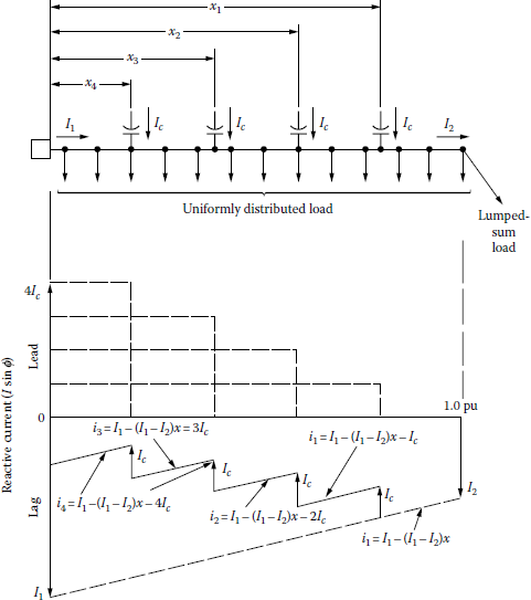
The optimum application of shunt capacitors on distribution feeders to reduce losses has been studied in numerous papers such as those by Neagle and Samson [5], Schmidt [7], Maxwell [8,9], Cook [10], Schmill [11], Chang [12–14], Bae [15], Gönen and Djavashi [17], and Grainger et al. [19,21–23]. Figure 8.21 shows a realistic representation of a feeder that contains a number of line segments with a combination of concentrated (or lumped-sum) and uniformly distributed loads, as suggested by Chang [13]. Each line segment represents a part of the feeder between sectionalizing devices, voltage regulators, and other points of significance. For the sake of convenience, the load or line current and the resulting 12R loss can be assumed to have two components, namely, (1) those due to the in-phase or active component of current and (2) those due to the out-of-phase or reactive component of current. Since losses due to the in-phase or active component of line current are not significantly affected by the application of shunt capacitors, they are not considered. This can be verified as follows.

Primary feeder with lumped-sum (or concentrated) and uniformly distributed loads and reactive current profile before adding the capacitor.
Assume that the 12R losses are caused by a lagging line current I flowing through the circuit resistance R. Therefore, it can be shown that
I2R=(Icosϕ)2R+(I sinϕ)2 R+(I sinϕ)2R(8.52)
After adding a shunt capacitor with current Ic, the resultants are a new line current I1 and a new power loss I21R. Hence,
I21R =(Icosϕ)2 R+(I sinϕ−Ic)2R(8.53)
Therefore, the loss reduction as a result of the capacitor addition can be found as
ΔPLS=I2R−I21R(8.54)
or by substituting Equations 8.56 and 8.57 into Equation 8.58,
ΔPLS=2(I sin ϕ)IcR−I2cR(8.55)
Thus, only the out-of-phase or reactive component of line current, that is, I sin Q, should be taken into account for I2R loss reduction as a result of a capacitor addition.
Assume that the length of a feeder segment is 1.0 pu length, as shown in Figure 8.21. The current profile of the line current at any given point on the feeder is a function of the distance of that point from the beginning of the feeder. Therefore, the differential I2R loss of a dx differential segment located at a distance x can be expressed as
dPLS=3[I1−(I1−I2)x]2Rdx(8.56)
Therefore, the total I2R loss of the feeder can be found as
PLS=1.0∫x=0dPLS=31.0∫x=0[I1−(I1−I2)x]2Rdx=(I21+I1I2+I22)R(8.57)
where
PLS is the total I2R loss of the feeder before adding the capacitor
I1 is the reactive current at the beginning of the feeder segment
I2 is the reactive current at the end of the feeder segment
R is the total resistance of the feeder segment
x is the per unit distance from the beginning of the feeder segment
8.8.1 Loss Reduction Due to Capacitor Allocation
8.8.1.1 Case 1: One Capacitor Bank
The insertion of one capacitor bank on the primary feeder causes a break in the continuity of the reactive load profile, modifies the reactive current profile, and consequently reduces the loss, as shown in Figure 8.22.

Therefore, the loss equation after adding one capacitor bank can be found as before:
P'LS=3x1∫x=0[I1−(I1−I2)x−Ic]2Rdx+3 1.0∫x=x1[I1−(I1−I2)x]2Rdx(8.58)
or
P'LS=(I21+I1I2+I22)R+3x1[(x1−2)I1Ic−x1I2Ic+I2c]R(8.59)
Thus, the per unit power loss reduction as a result of adding one capacitor bank can be found from
ΔPLS=PLS−P'LSPLS(8.60)
or substituting Equations 8.57 and 8.58 into Equation 8.60,
ΔPLS=−3x1[(x1−2)I1I2Ic+I2c]R(I21+I1I2+I22)R(8.61)
or rearranging Equation 8.61 by dividing its numerator and denominator by /j2 so that
ΔPLS=3x11+(I2/I1)+(I2/I1)2[(2−x1(IcI1)+x1(I2I1)(IcI1)−(IcI1)2](8.62)
If c is defined as the ratio of the capacitive kilovoltamperes (ckVAs) of the capacitor bank to the total reactive load, that is,
c=ckVA of capacitor installedTotal reactive load(8.63)
then
c=IcI1(8.64)
and if λ is defined as the ratio of the reactive current at the end of the line segment to the reactive current at the beginning of the line segment, that is,
λ=Reactive current at the end of line segmentReactive current at the beginning of line segment(8.65)
then
λ=I2I1(8.66)
Therefore, substituting Equations 8.64 and 8.66 into Equation 8.62, the per unit power loss reduction can be found as
ΔPLS=3x11+λ+λ2[(2−x1)c+x1λc−c2](8.67)
or
ΔPLS=3cx11+λ+λ2[(2−x1)+x1λ−c](8.68)
where x1 is the per unit distance of the capacitor-bank location from the beginning of the feeder segment (between 0 and 1.0 pu).
If a is defined as the reciprocal of 1 + λ + λ2, that is,
α=11+λ+λ2(8.69)
then Equation 8.68 can also be expressed as
ΔPLS=3αcx1[(2−x1)+λx1−c](8.70)
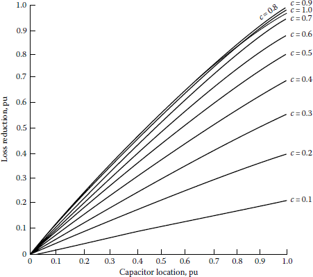
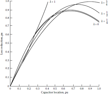
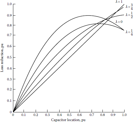
Figures 8.23, 8.24, 8.25, 8.26 and 8.27 give the loss reduction that can be accomplished by changing the location of a single capacitor bank with any given size for different capacitor compensation ratios along the feeder for different representative load patterns, for example, uniformly distributed loads (λ = 0), concentrated or lumped-sum loads (λ = 1), or a combination of concentrated and uniformly distributed loads (0 < λ < 1). To use these nomographs for a given case, the following factors must be known:
- Original losses due to the reactive current
- Capacitor compensation ratio
- The location of the capacitor bank

Loss reduction as a function of the capacitor-bank location and capacitor compensation ratio for a line segment with uniformly distributed loads (λ = 0).

Loss reduction as a function of the capacitor-bank location and capacitor compensation ratio for a line segment with a combination of concentrated and uniformly distributed loads (λ = 1/4).

Loss reduction as a function of the capacitor-bank location and capacitor compensation ratio for a line segment with a combination of concentrated and uniformly distributed loads (λ = 1/2).
Loss reduction as a function of the capacitor-bank location and capacitor compensation ratio for a line segment with a combination of concentrated and uniformly distributed loads (λ = 3/4).

Loss reduction as a function of the capacitor-bank location and capacitor compensation ratio for a line segment with concentrated loads (λ = 1).
As an example, assume that the load on the line segment is uniformly distributed and the desired compensation ratio is 0.5. From Figure 8.23, it can be found that the maximum loss reduction can be obtained if the capacitor bank is located at 0.75 pu length from the source. The associated loss reduction is 0.85 pu or 85%. If the bank is located anywhere else on the feeder, however, the loss reduction would be less than the 85%.
In other words, there is only one location for any given-size capacitor bank to achieve the maximum loss reduction. Table 8.5 gives the optimum location and percent loss reduction for a givensize capacitor bank located on a feeder with uniformly distributed load (λ = 0). From the table it can be observed that the maximum loss reduction can be achieved by locating the single capacitor bank at the two-thirds length of the feeder away from the source. Figure 8.28 gives the loss reduction for a given capacitor bank of any size and located at the optimum location on a feeder with various combinations of load types based on Equation 8.70. Figure 8.29 gives the loss reduction due to an optimum-sized capacitor bank located on a feeder with various combinations of load types.
Loss reduction due to a capacitor bank located at the optimum location on a line section with various combinations of concentrated and uniformly distributed loads.
Loss reduction due to an optimum-sized capacitor bank located on a line segment with various combinations of concentrated and uniformly distributed loads.
Optimum Location and Optimum Loss Reduction
Capacitor-Bank Rating, pu |
Optimum Location, pu |
Optimum Loss Reduction, % |
|---|---|---|
0.0 |
1.0 |
0 |
0.1 |
0.95 |
27 |
0.2 |
0.90 |
49 |
0.3 |
0.85 |
65 |
0.4 |
0.80 |
77 |
0.5 |
0.75 |
84 |
0.6 |
0.70 |
88 |
0.7 |
0.65 |
89 |
0.8 |
0.60 |
86 |
0.9 |
0.55 |
82 |
1.0 |
0.50 |
75 |
8.8.1.2 Case 2: Two Capacitor Banks
Assume that two capacitor banks of equal size are inserted on the feeder, as shown in Figure 8.30. The same procedure can be followed as before, and the new loss equation becomes
P'LS=3x1∫x=0[I1−(I1−I2)x−2Ic]2Rdx+3x2∫x=x1[I1−(I1I2)x−Ic]2Rdx+31.0∫x=x2[I1−(I1−I2)x]2Rdx(8.71)

Therefore, substituting Equations 8.57 and 8.71 into Equation 8.60, the new per unit loss reduction equation can be found as
ΔPLS=3αcx1[(2−x1)+λx1−3c]+3αcx2[(2−x2)+λx2−c](8.72)
or
ΔPLS=3αc{x1[(2−x1)+λx1−3c]+x2[(2−x2)+λx2−c]}(8.73)
8.8.1.3 Case 3: Three Capacitor Banks
Assume that three capacitor banks of equal size are inserted on the feeder, as shown in Figure 8.31. The relevant per unit loss reduction equation can be found as
ΔPLS=3αc{x1[(2−x1)+λx1−5c]+x2[(2−x2)+λx2−3c]+x3[(2−x3)+λx3−c]}(8.74)

8.8.1.4 Case 4: Four Capacitor Banks
Assume that four capacitor banks of equal size are inserted on the feeder, as shown in Figure 8.32. The relevant per unit loss reduction equation can be found as
ΔPLS=3αc{x1[(2−x1)+λx1−7c]+x2[(2−x2)+λx2−5c]+x3[(2−x3)+λx3−3c]+x4[(2−x4)λx4−c]}(8.75)
8.8.1.5 Case 5: n Capacitor Banks
As the aforementioned results indicate, the per unit loss reduction equations follow a definite pattern as the number of capacitor banks increases. Therefore, the general equation for per unit loss reduction, for an n capacitor-bank feeder, can be expressed as
PLS=3αcn∑i=1xi[(2−xi)+λxi−(2i−1)c](8.76)
where
c is the capacitor compensation ratio at each location (determined from Equation 8.63)
xi is the per unit distance of the ith capacitor-bank location from the source
n is the total number of capacitor banks
8.8.2 Optimum Location of a Capacitor Bank
The optimum location for the ¿th capacitor bank can be found by taking the first-order partial derivative of Equation 8.76 with respect to xi and setting the resulting expression equal to zero. Therefore,
xi,opt=11−λ−(2i−1)c2(1−λ)(8.77)
where xi,opt is the optimum location for the ith capacitor bank in per unit length.
By substituting Equation 8.81 into Equation 8.80, the optimum loss reduction can be found as
PLS,opt=3αcn∑i=1[11−λ−(2i−1)c(1−λ)+i2c21−λ−c24(1−λ)−ic21−λ](8.78)
Equation 8.78 is an infinite series of algebraic form that can be simplified by using the following relations:
n∑i=1(2i−1)=n2(8.79)
n∑i=1i=n(n+1)2(8.80)
n∑i=1i2=n(n+1)(2n+1)6(8.81)
n∑i=111−λ=n1−λ(8.82)
Therefore,
PLS,opt=3αcn∑i=1[n1−λ−n2c1−λ+nc2(n+1)(2n+1)6−nc24(1−λ)−nc2(n+1)2(1−λ)](8.83)
PLS,opt=3αc1−λ[n−cn2+c2n(4n2−1)12](8.84)
The capacitor compensation ratio at each location can be found by differentiating Equation 8.88 with respect to c and setting it equal to zero as
c=22n+1(8.85)
Equation 8.86 can be called the 2/(2n + 1) rule. For example, for n = 1, the capacitor rating is two-thirds of the total reactive load that is located at
x123(1−λ)(8.86)
of the distance from the source to the end of the feeder, and the peak loss reduction is
ΔPLS,opt=22(1−λ)(8.87)
For a feeder with a uniformly distributed load, the reactive current at the end of the line is zero (i.e., I2 = 0); therefore,
Thus, for the optimum loss reduction of
the optimum value of x1 is
and the optimum value of c is
Figure 8.33 gives a maximum loss reduction comparison for capacitor banks, with various total reactive compensation levels and located optimally on a line segment that has uniformly distributed load (λ = 0), based on Equation 8.84. The given curves are for one, two, three, and infinite number of capacitor banks.

Comparison of loss reduction obtainable from n = 1, 2, 3, and ∞ number of capacitor banks, with λ = 0.
For example, from the curve given for one capacitor bank, it can be observed that a capacitor bank rated two-thirds of the total reactive load and located at two-thirds of the distance out on the feeder from the source provides for a loss reduction of 89%. In the case of two capacitor banks, with four-fifths of the total reactive compensation, located at four-fifths of the distance out on the feeder, the maximum loss reduction is 96%. Figure 8.34 gives similar curves for a combination of concentrated and uniformly distributed loads (λ = 1/4).

Comparison of loss reduction obtainable from n = 1, 2, 3, 4, and ∞ number of capacitor banks, with λ = 1/4.
8.8.3 Energy Loss Reduction Due to Capacitors
The per unit energy loss reduction in a three-phase line segment with a combination of concentrated and uniformly distributed loads due to the allocation of fixed shunt capacitors is
where
is the reactive load factor = Q/S
T is the total time period during which fixed-shunt-capacitor banks are connected
ΔEL is the energy loss reduction, pu
The optimum locations for the fixed shunt capacitors for the maximum energy loss reduction can be found by differentiating Equation 8.91 with respect to xi and setting the result equal to zero. Therefore,
The optimum capacitor location for the maximum energy loss reduction can be found by setting Equation 8.92 to zero, so that
Similarly, the optimum total capacitor rating can be found as
From Equation 8.95, it can be observed that if the total number of capacitor banks approaches infinity, then the optimum total capacitor rating becomes equal to the reactive load factor.
If only one capacitor bank is used, the optimum capacitor rating to provide for the maximum energy loss reduction is
This equation gives the well-known two-thirds rule for fixed shunt capacitors. Figure 8.35 shows the relationship between the total capacitor compensation ratio and the reactive load factor, in order to achieve maximum energy loss reduction, for a line segment with uniformly distributed load where λ = 0 and α = 1.

Relationship between the total capacitor compensation ratio and the reactive load factor for uniformly distributed load (λ = 0 and α = 1).
By substituting Equation 8.94 into Equation 8.95, the optimum energy loss reduction can be found as
where CT is the total reactive compensation level = cn.
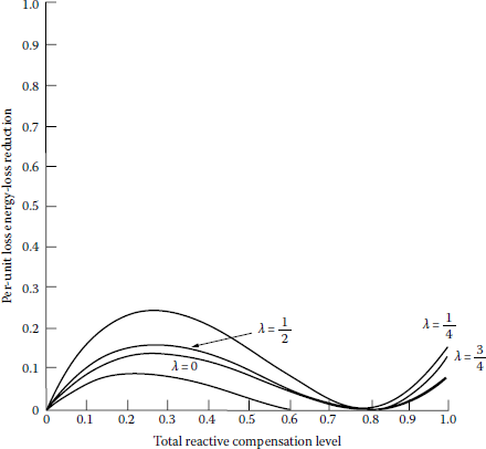
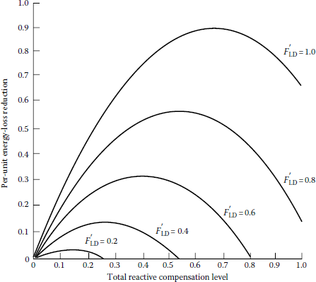
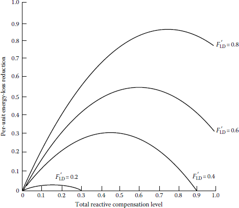
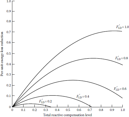
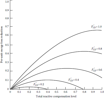
Based on Equation 8.97, the optimum energy loss reductions with any size capacitor bank located at the optimum location for various reactive load factors have been calculated, and the results have been plotted in Figures 8.36, 8.37, 8.38, 8.39 and 8.40. It is important to note the fact that, for all values of λ, when reactive load factors are 0.2 or 0.4, the use of a fixed capacitor bank with corrective ratios of 0.4 and 0.8, respectively, gives a zero energy loss reduction.

Energy loss reduction with any capacitor-bank size, located at optimum location ( = 0.2).
Energy loss reduction with any capacitor-bank size, located at the optimum location ( = 0.4).

Energy loss reduction with any capacitor-bank size, located at the optimum location ( = 0.6).

Energy loss reduction with any capacitor-bank size, located at the optimum location ( = 0.6).
Energy loss reduction with any capacitor-bank size, located at the optimum location ( = 0.6).
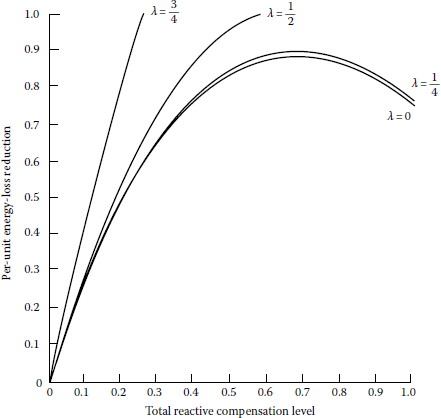
Figures 8.41, 8.42, 8.43, 8.44 and 8.45 show the effects of various reactive load factors on the maximum energy loss reductions for a feeder with different load patterns.
Effects of reactive load factors on energy loss reduction due to capacitor-bank installation on a line segment with uniformly distributed load (λ = 0).
Effects of reactive load factors on energy loss reduction due to capacitor-bank installation on a line segment with a combination of concentrated and uniformly distributed loads (λ = 1/4).

Effects of reactive load factors on energy loss reduction due to capacitor-bank installation on a line segment with a combination of concentrated and uniformly distributed loads (λ = 1/2).
Effects of reactive load factors on loss reduction due to capacitor-bank installation on a line segment with a combination of concentrated and uniformly distributed loads (λ = 3/4).
Effects of reactive load factors on energy loss reduction due to capacitor-bank installation on a line segment with a concentrated load (λ = 1).
8.8.4 Relative Ratings of Multiple Fixed Capacitors
The total savings due to having two fixed-shunt-capacitor banks located on a feeder with uniformly distributed load can be found as
or
where
K1 is the a constant to convert energy loss savings to dollars, $/kWh
K2 is the a constant to convert power loss savings to dollars, $/kWh
Since the total capacitor-bank rating is equal to the sum of the ratings of the capacitor banks,
or
By substituting Equation 8.101 into Equation 8.99,
The optimum rating of the second fixed capacitor bank as a function of the total capacitor-bank rating can be found by differentiating Equation 8.106 with respect to c2, so that
and setting the resultant equation equal to zero,
and since
then
The result shows that if multiple fixed-shunt-capacitor banks are to be employed on a feeder with uniformly distributed loads, in order to receive the maximum savings, all capacitor banks should have the same rating.
8.8.5 General Savings Equation for Any Number of Fixed Capacitors
From Equations 8.76 and 8.92, the total savings equation in a three-phase primary feeder with a combination of concentrated and uniformly distributed loads can be found as
where
K1 is the constant to convert energy loss savings to dollars, $/kWh
K2 is the constant to convert power loss savings to dollars, $/kWh
K3 is the constant to convert total fixed capacitor ratings to dollars, $/kvar
xi is the ith capacitor location, pu length
n is the total number of capacitor banks
is the reactive load factor
CT is the total reactive compensation level
c is the capacitor compensation ratio at each location
λ is the ratio of reactive current at the end of the line segment to the reactive load current at the beginning of the line segment
T is the total time period during which fixed-shunt-capacitor banks are connected
By taking the first- and second-order partial derivatives of Equation 8.107 with respect to x1,
and
Setting Equation 8.108 equal to zero, the optimum location for any fixed capacitor bank with any rating can be found as
where 0 ≤ xi ≤ 1.0 pu length. Setting the capacitor bank anywhere else on the feeder would decrease rather than increase the savings from loss reduction.
Some of the cardinal rules that can be derived for the application of capacitor banks include the following:
- The location of fixed shunt capacitors should be based on the average reactive load.
- There is only one location for each size of capacitor bank that produces maximum loss reduction.
- One large capacitor bank can provide almost as much savings as two or more capacitor banks of equal size.
- When multiple locations are used for fixed-shunt-capacitor banks, the banks should have the same rating to be economical.
- For a feeder with a uniformly distributed load, a fixed capacitor bank rated at two-thirds of the total reactive load and located at two-thirds of the distance out on the feeder from the source gives an 89% loss reduction.
- The result of the two-thirds rule is particularly useful when the reactive load factor is high. It can be applied only when fixed shunt capacitors are used.
- In general, particularly at low reactive load factors, some combination of fixed and switched capacitors gives the greatest energy loss reduction.
- In actual situations, it may be difficult, if not impossible, to locate a capacitor bank at the optimum location; in such cases the permanent location of the capacitor bank ends up being suboptimum.
8.9 Further Thoughts on Capacitors and Improving Power Factors
In a given circuit, when the relative current is reduced, the total current is reduced. If the real current does not change, which is usually the case, the power factor will improve as reactive current is reduced. When the reactive current becomes zero, all the current becomes the real current, and thus, the power factor will be equal to 1.0, that is, unity, or 100%. For instance, in Figure 8.46a, if a capacitor is installed to supply the total reactive power, or 60 kvar, the line power factor may be improved by supplying the load reactive power requirements by a capacitor.
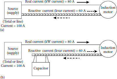
Schematic diagram for the use of capacitors to reduce total line current by supplying reactive power locally: (a) without the use of capacitors and (b) with the use of capacitors.
In an induction load or equipment (e.g., induction motor) the real power is supplied and lost, whereas the reactive power is supplied and not lost. Here, the reactive power is used to store energy in the motor’s magnetic energy field. Since the current is alternating, the magnetic field undergoes cycles of building up and breaking down. When the current is breaking down, the reactive current flows out of the motor back to the supply, as shown in Figure 8.46a. Note that the flow of the real power is unidirectional, that is, from the source to the motor. However, it is possible to provide only real power from the power source and provide the necessary reactive power from a capacitor.
Note that contrary to the real power flow (which is unidirectional), the reactive power flow is cyclic in nature, that is, flows out of capacitor to the motor and then flows back to the capacitor, as illustrated in Figure 8.46b. Here, the capacitor acts as a temporary storage area for the reactive power by storing energy units in electric field.
Figure 8.46 illustrates how to provide reactive power alternatively by the use of capacitors locally. Notice that the working load requires 80 A, but due to the magnetic requirements of the motor of 60 A, the supply circuit must carry 100 A. After the installation of the capacitor, the necessary magnetic requirements of the motor are supplied by the capacitor. Thus, the supply circuit needs to deliver only 80 A to do exactly the same work. The supply circuit is now carrying only kilowatts, so no system capacity is wasted in carrying the so-called non-working current.
Also, it can be observed from the power triangle that the simple subtraction of real power from total apparent power never equals the reactive power except at unity power factor.
However, in actual practice, it is generally not necessary nor economical to improve the power factor to 100%. Because of this fact, the utility companies provide the power factor of about 0.95 at their power plants. The remainder is supplied by using overexcited synchronous motors orating with no loads, or capacitor banks.
8.10 Capacitor Tank-Rupture Considerations
When the total energy input to the capacitor is larger than the strength of the tank’s envelope to withstand such input, the tank of the capacitor ruptures. This energy input could happen under a wide range of current–time conditions. Through numerous testing procedures, capacitor manufacturers have generated tank–rupture curves as a function of fault current available.
The resulting tank–rupture time–current characteristic curves with which fuse selection is coordinated have furnished comparatively good protection against tank rupture. Figure 8.47 shows the results of tank–rupture tests conducted on all-film capacitors. Figure 8.48 shows the capacitor reliability cycle during its lifetime. The longer it takes for the dielectric material to wear out due to the forces generated by the combination of electric stress and temperature, the greater is its reliability. In other words, the wear-out process or time to failure is a measure of life and reliability. Currently, there are numerous methods that can be used to detect the capacitor tank ruptures. Burrage [24] categorizes them as follows:
- Detection of sound produced by the rupture
- Observation of smoke and/or vapor from the capacitor tank upon rupture
- Observation of ultraviolet light generated by the arc getting outside the capacitor tank
- Measurement of the change in arc voltage when the capacitor tank is breached
- Detection of a sudden reduction in internal pressure
- Measurement of the distortion generated by gas pressure within the capacitor tank

Time-to-rupture characteristics for 200 kvar 7.2 kV all-film capacitors.
(From McGraw-Edison Company, The ABC of Capacitors, Bulletin R230-90-1, 1968.)

Capacitor reliability cycle.
(From McGraw-Edison Company, The ABC of Capacitors, Bulletin R230-90-1, 1968.)
8.11 Dynamic Behavior of Distribution Systems
The characteristics of the distribution system dynamic behavior include (1) fault effects and transient recovery voltage (TRV), (2) switching and lightning surges, (3) inrush and cold-load current transients, (4) ferroresonance, and (5) harmonics.
In the event of a fault on a distribution system, there will be a substantial change in current magnitude on the faulted phase. It is also possible for the current to have a dc offset that is a function of the voltage wave at the time of the fault and the X/R ratio of the circuit. This may cause a voltage rise on the unfaulted phases due to neutral shift that results in saturation of transformers and increased load current magnitudes.
On the other hand, it may cause a reduction in voltage and load current on the faulted phase. When a circuit recloser clears the fault at a current zero, a higher-frequency transient voltage is superimposed on the power frequency recovery voltage. The resultant voltage is called the TRV. It is possible to have its crest magnitudes be two or three times the nominal system voltage. This may cause failure to clear or restrike that may produce substantial switching surges.
Switching surges are generated when loads, station capacitor banks, or feeders are energized or reenergized; or when faults are initiated, cleared, and reinitiated. The factors affecting the magnitude and duration of the resultant voltage transients include (1) the system impedance characteristics, (2) the amount of capacitive kilovars connected at the time of switching, (3) the location of the capacitor bank on the system, (4) the type of breaker, and (5) the breaker poleclosing angles. In general, the switching surges on distribution systems have not been taken seriously so far.
However, if the current trend toward higher-distribution voltage levels and reduced insulation levels continues, this may change. But voltage surges resulting from lightning strokes to the distribution line will usually require the most severe design requirements. The factors affecting the lightning surge include (1) the system configuration and the system grounding and shielding, (2) the stroke characteristics and stroke location, (3) the sparkover of arresters remote from the converters, (4) the amount of the connected capacitive kilovars in the surge path, and (5) the loss mechanism (corona, skin effect) in the surge path.
The energization of motors, transformers, capacitors, feeders, and loads generates current transients. For example, when motors and other loads draw high starting currents, capacitors draw a high-frequency inrush based on the instantaneous voltage and the circuit inductance as well as the capacitance, whereas in a transformer the magnitude of this inrush depends upon the voltage wave at the time of energization and the residual flux in the core.
It is important to recognize the fact that low voltage during inrush can harm equipment involved and stop the circuit from recovering without sectionalizing. Furthermore, protective devices may operate incorrectly or not operate due to the high-magnitude and high-frequency currents.
8.11.1 Ferroresonance
Ferroresonance is an oscillatory phenomenon caused by the interaction of system capacitance with the nonlinear inductance of a transformer. These capacitive and inductive elements make a seriesresonant circuit that can generate high transient or sustained overvoltages that can damage system equipment.
These overvoltages are more likely to take place where a considerable length of cable is connected to an overloaded three-phase transformer (or bank) and single-phase switching is done at a point remote from the transformer (e.g., riser pole). Serious damage to equipment may be prevented by recognizing the conditions that increase the probability of these overvoltages and taking appropriate preventive measures.
The more serious overvoltages may be evidenced by (1) flashover or damage to lightning arresters, (2) transformer humming with only one phase closed, (3) damage to transformers and other equipment, (4) three-phase motor reversals, and (5) high secondary voltages.
Even though the ferroresonant phenomenon has been recognized for some time, until recently it has not been considered as a serious operating problem on electric distribution systems. Changes in the characteristics of distribution systems and in transformer design have resulted in the increased probability of ferroresonant overvoltages when switching three-phase transformer installations.
For example, the capacitance of cable is much greater (i.e., capacitive reactance lower) than that of open wire, and present trends are toward a greater use of underground cables due to the esthetic considerations. Also, system operation at higher than nominal voltages and trends in transformer design have led to the operation of distribution transformer cores at higher saturation.
Furthermore, the use of higher-distribution voltages results in distribution transformers with greater magnetizing reactance. At the same time, underground system capacitance will be greater (capacitive reactance lower).
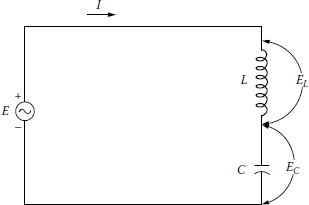
Consider the LC circuit shown in Figure 8.49. Note that the resistance is neglected for the sake of simplicity. If the inductive reactance XL of the inductor is equal in magnitude to the capacitive reactance XC of the capacitor, the circuit is in resonance. The voltage E across the inductor is 180° out of phase with the voltage EC across the capacitor. The voltages EL and EC can be expressed as
and
Example 8.20
Consider a downtown 34.5 kV underground cable, and for the purpose of illustration, assume that XL/XC = 0.9 in the LC circuit given by Figure 8.49, and therefore, XC/XL = 1.1111. If the line-to-line voltage is 34.5 kV, determine
- The voltages EL
- The voltages EC
Solution
-
or
In practice, such situation often takes place in downtown underground networks when a 34.5 kV underground cable feeds a transformer. As a result of the ferroresonance (because of the XL of the transformer and XC of the cable), the 34.5 kV underground cable breaks down due to such high voltages, causing a short-circuit condition. The fault usually takes place at the entrance terminal to the transformer. It has often puzzled some of the protection engineers. Thus, in such situations, it is a good idea to check for possible ferroresonance conditions.
-
or
Therefore, in this case the voltage across the capacitor is 10 times the source voltage. The nearer the circuit is to the actual resonance, the greater will be the overvoltage.
Although the previous text is a relatively simple example of a resonant circuit, the basic concept is very similar to ferroresonance with one notable exception. In a ferroresonant circuit the capacitor is in series with a nonlinear (iron-core) inductor. A plot of the voltampere or impedance characteristic of an iron-core reactor would have the same general shape as the BH curve of the iron core. If the iron-core reactor is operating at a point near saturation, a small increase in voltage can cause a large decrease in the effective inductive reactance of the reactor. Therefore, the value of inductive reactance can vary widely and resonance can occur over a range of capacitance values. The effects of ferroresonance can be minimized by such measures as
- Using grounded-wye–grounded-wye transformer connection
- Using open-wye–open-delta transformer connection
- Using switches rather than fuses at the riser pole
- Using single-pole devices only at the transformer location and three-pole devices for remote switching
- Avoiding switching an unloaded transformer bank at a point remote from the transformers
- Keeping XC/XM ratios high (10 or more)
- Installing neutral resistance
- Using dummy loads to suppress ferroresonant overvoltages
- Assuring load is present during switching
- Using larger transformers
- Limiting the length of cable serving the three-phase installation
- Using only three-phase switching and sectionalizing devices at the terminal pole
- Temporarily grounding the neutral of a floating-wye primary during switching operations
8.11.2 Harmonics on Distribution Systems
The power industry has recognized the problem of power system harmonics since the 1920s when distorted voltage and current waveforms were observed on power lines. However, the levels of harmonics on distribution systems have generally been insignificant in the past.
Today, it is obvious that the levels of harmonic voltages and currents on distribution systems are becoming a serious problem. Some of the most important power system operational problems caused by harmonics have been reported to include the following [25]:
- Capacitor-bank failure from dielectric breakdown or reactive power overload
- Interference with ripple control and power-line carrier systems, causing misoperation of systems that accomplish remote switching, load control, and metering
- Excessive losses in—and heating of—induction and synchronous machines
- Overvoltages and excessive currents on the system from resonance to harmonic voltages or currents on the network
- Dielectric instability of insulated cables resulting from harmonic overvoltages on the system
- Inductive interference with telecommunication systems
- Errors in induction watthour meters
- Signal interference and relay malfunction, particularly in solid-state and microprocessorcontrolled systems
- Interference with large motor controllers and power plant excitation systems (reported to cause motor problems as well as nonuniform output)
These effects depend, of course, on the harmonic source, its location on the power system, and the network characteristics that promote propagation of harmonics. There are numerous sources of harmonics. In general, the harmonic sources can be classified as (1) previously known harmonic sources and (2) new harmonic sources. The previously known harmonic sources include the following:
- Tooth ripples or ripples in the voltage waveform of rotating machines
- Variations in air-gap reluctance over synchronous machine pole pitch
- Flux distortion in the synchronous machine from sudden load changes
- Nonsinusoidal distribution of the flux in the air gap of synchronous machines
- Transformer magnetizing currents
- Network nonlinearities from loads such as rectifiers, inverters, welders, arc furnaces, voltage controllers, frequency converters
While the established sources of harmonics are still present on the system, the power network is also subjected to new harmonic sources:
- Energy conservation measures, such as those for improved motor efficiency and load matching, which employ power semiconductor devices and switching for their operation. These devices often produce irregular voltage and current waveforms that are rich in harmonics.
- Motor control devices such as speed controls for traction.
- High-voltage dc power conversion and transmission.
- Interconnection of wind and solar power converters with distribution systems.
- Static-var compensators that have largely replaced synchronous condensors as continuously variable-var sources.
- The development and potentially wide use of electric vehicles that require a significant amount of power rectification for battery charging.
- The potential use of direct energy conversion devices, such as magnetohydrodynamics, storage batteries, and fuel cells, that require dc/ac power converters.
The presence of harmonics causes the distortion of the voltage or current waves. The distortions are measured in terms of the voltage or current harmonic factors. The IEEE Standard 519-1981 [26] defines the harmonic factors as the ratio of the root-mean-square value of all the harmonics to the rootmean-square value of the fundamental. Therefore, the voltage harmonic factor HFv can be expressed as
and the current harmonic factor HFI can be expressed as
The presence of the voltage distortion results in harmonic currents. Figure 8.50 shows harmonic analysis of a peaked no-load current wave.

The characteristics of harmonics on a distribution system are functions of both the harmonic source and the system response. For example, utilities are presently installing more and larger transformers to meet ever-increasing power demands. Each transformer is a source of harmonics to the distribution system.
Furthermore, these transformers are being operated closer to the saturation point. Transformer saturation results in a nonsinusoidal exciting current in the iron core when a sinusoidal voltage is applied. The level of transformer saturation is affected by the magnitude of the applied voltage.
When the applied voltage is above the rated voltage, the harmonic components of the exciting current increase dramatically. Owen [27] has demonstrated this for a typical substation power transformer, as shown in Figure 8.51. Also, some utility companies are overexciting distribution transformers as a matter of policy and practice, which compounds the harmonic problem.

Harmonic components of transformer exciting current.
(From Owen, R.E., Distribution system harmonics: Effects on equipment and operation, Pacific Coast Electrical Association Engineering and Operating Conference, Los Angeles, CA, March 15–16, 1979.)
The current harmonics of consequence that are produced by transformers are generally in the order of the third, fifth, and seventh. Table 8.6 gives a summary of the conditions obtaining third harmonics with different connections of double-wound three-phase transformers. The table is prepared for third harmonics in double-wound single-phase core- and shell-type transformers and in three-phase shelltype transformers for three-phase service. Figure 8.52 shows the shape of the resultant waves obtained when combining the fundamental and third harmonic along with different positions of the harmonic.

Combinations of fundamental and third-harmonic waves: (a) harmonic in phase, (b) harmonic 90° leading, (c) harmonic in opposition, and (d) harmonic 90° lagging.
(From Stigant, S.A. and Franklin, A.C., The J&P Transformer Book, Butterworth, London, U.K., 1973.)
The Influence of Three-Phase Transformer Connections on Third Harmonics
Connectionsa |
Primary |
Flux |
Secondary |
||||||
|---|---|---|---|---|---|---|---|---|---|
Currents |
Voltages |
Currents |
Voltages |
||||||
No-Load |
Line |
Line |
Phase |
No-Load |
Line |
Line |
Phase |
||
1. Wye I.N./wye I.N. |
Sine |
Sine |
Sine |
Contains 3d h(P) |
Contains 3d h(FT) |
Sine |
Sine |
Contains 3d h(P) | |
2. Wye N. to G./wye I.N. |
Contains 3d h(P)b |
Contains 3d h(P)b |
Sine |
Contains 3d h(P)b |
Contains 3d h(FT)b |
Sine |
Sine |
Contains 3d h(P)b | |
3. Wye I.N./wye, four-wire |
Sine |
Sine |
Sine |
Contains 3d h(P)b |
Contains 3d h(FT)b |
Contains 3d h(P)b |
Contains 3d h(P)b |
Sine |
Contains 3d h(P)b |
4. Wye I.N. tertiary delta/wye I.N. |
Sine in star, 3d h in delta (P) |
Sine |
Sine |
Sine |
Sine |
Sine |
Sine |
Sine | |
5. Wye I.N./delta |
Sine |
Sine |
Sine |
Sine |
Sine |
Contains 3d h(P) |
Sine |
Sine |
Sine |
6. Wye N. to G./delta |
Contains 3d h(P)b |
Contains 3d h(P)b |
Sine |
Sine |
Sine |
Contains 3d h(P)b |
Sine |
Sine |
Sine |
7. Wye I.N./interconnected wye I.N. |
Sine |
Sine |
Sine |
Contains 3d h(P) |
Contains 3d h(FT) |
Sine |
Sine |
Sine | |
8. Wye I.N./interconnected wye, four-wire |
Sine |
Sine |
Sine |
Contains 3d h(P) |
Contains 3d h(FT) |
Sine |
Sine |
Sine | |
9. Delta/wye I.N. |
Contains 3d h(P) |
Sine |
Sine |
Sine |
Sine |
Sine |
Sine |
Sine | |
10. Delta/wye, four-wire |
Contains 3d h(P) |
Sine |
Sine |
Sine |
Sine |
Contains 3d h(P) |
Contains 3d h(P) |
Sine |
Sine |
11. Delta/delta |
Contains 3d h(P) |
Sine |
Sine |
Sine |
Sine |
Contains 3d h(P)b |
Sine |
Sine |
Sine |
Source: Stigant, S.A. and Franklin, A.C., The J&P Transformer Book, Butterworth, London, U.K., 1973.
a I.N., isolated neutral; N. to G., transformer primary neutral connected to generator neutral; (P), peaked wave; (FT), flat-top wave.
b In all these cases the third-harmonic component is less than it otherwise would be if (1) the circulating third-harmonic current flowed through a closed delta winding only or (2) the neutral point was isolated.
Note that at harmonic frequencies the phase angles (due to the various harmonic impedances of each load) can be anything between 0° and 360°. Also, as the harmonic order increases, the power-line impedance itself plays the role of a controlling factor, and therefore, the harmonic current will have different phase angles at different locations.
The impact of harmonics on transformers is numerous. For example, voltage harmonics result in increased iron losses; current harmonics result in increased copper losses and stray flux losses. The losses may in turn cause the transformer to be overheated.
The harmonics may also cause insulation stresses and resonances between transformer windings and line capacitances at the harmonic frequencies. The total eddy-current losses are proportional to the harmonic frequencies and can be expressed as
where
TECL is the total eddy-current loss
ECL1 is the eddy-current loss at rated fundamental current
h is the harmonic order
I1 is the rated fundamental current
Ih is the harmonic current
Capacitor-bank sizes and locations are critical factors in a distribution system’s response to harmonic sources. The combination of capacitors and the system reactance causes both seriesand parallel-resonant frequencies for the circuit.
The possibility of resonance between a shunt capacitor bank and the rest of the system, at a harmonic frequency, may be determined by calculating equal order of harmonic h at which resonance may take place [29]. This equal order of harmonic is found from
where
Ssc is the short-circuit power of a system at the point of application, MVA
Qcap is the capacitor-bank size, Mvar
The parallel-resonant frequency fp can be expressed as
Substituting Equation 8.120 into Equation 8.121,
or
or
where
f1 is the fundamental frequency, Hz
Xcap is the reactance of capacitor bank, pu or Ω
Xsc is the reactance of power system, pu or Ω
Lsc is the inductance of power system, H
C is the capacitance of capacitor bank, F
The effects of the harmonics on the capacitor bank include (1) overheating of the capacitors, (2) overvoltage at the capacitor bank, (3) changed dielectric stress, and (4) losses in capacitors. According to Kimbark [29], the increase of losses in capacitors due to harmonics can be expressed as
where
LCDH is the losses in capacitors due to harmonics
C is the capacitance
(tan δ)h is the loss factor at frequency of the hth harmonic
Wh = 2π times frequency of the hth harmonic
Vh is the rms voltage of the hth harmonic
The harmonic control techniques include (1) locating the capacitor banks strategically, (2) selecting capacitor-bank sizes properly, (3) ungrounding or deleting the capacitor bank, (4) using shielded cables, (5) controlling grounds properly, and (6) using harmonic filters.
Problems
-
8.1 Assume that a feeder supplies an industrial consumer with a cumulative load of (1) induction motors totaling 300 hp that run at an average efficiency of 89% and a lagging average power factor of 0.85, (2) synchronous motors totaling 100 hp with an average efficiency of 86%, and (3) a heating load of 100 kW. The industrial consumer plans to use the synchronous motors to correct its overall power factor. Determine the required power factor of the synchronous motors to correct the overall power factor at peak load to
- Unity
- 0.96 lagging
-
8.2 A 2.4/4.16 kV wye-connected feeder serves a peak load of 300 A at a lagging power factor of 0.7 connected at the end of the feeder. The minimum daily load is approximately 135 A at a power factor of 0.62. If the total impedance of the feeder is 0.50 + j1.35 Ω, determine the following:
- The necessary kilovar rating of the shunt capacitors located at the load to improve the peak-load power factor to 0.96
- The reduction in kilovoltamperes and line current due to the capacitors
- The effects of the capacitors on the voltage regulation and voltage drop in the feeder
- The power factor at minimum daily load level
-
8.3 Assume that a locked-rotor starting current of 90 A at a lagging load factor of 0.30 is supplied to a motor that is operated discontinuously. A normal operating current of 15 A, at a lagging power factor of 0.80, is drawn by the motor from the 2.4/4.16 kV feeder of Problem 8.2. Assume that a series capacitor is desired to be installed in the feeder to improve the voltage regulation and limit lamp flicker from the intermittent motor starting, and determine the following:
- The voltage dip due to the motor starting, before the installation of the series capacitor
- The necessary size of the capacitor to restrict the voltage dip at motor start to not more than 3%
-
8.4 Assume that a three-phase distribution substation transformer has a nameplate rating of 7250 kVA and a thermal capability of 120%. If the connected load is 8816 kVA with a 0.85 lagging power factor, determine the following:
- The kilovar rating of the shunt capacitor bank required to decrease the kilovoltampere load on the transformer to its capability level
- The power factor of the corrected load
- The kilovar rating of the shunt capacitor bank required to correct the load power factor to unity
- The corrected kilovoltampere load at this unity power factor
-
8.5 Assume that the NP&NL Utility Company is presently operating at 90% power factor. It is desired to improve the power factor to 98%. To study the power factor improvement, a number of load flow runs have been made and the results are summarized in the following table. Using the relevant additional information given in Table P8.5, repeat Example 8.19.
Summary of Load Flows
Comment
At 90% PF
At 99% PF
Total loss reduction due to capacitors applied to substation buses, kW
496
488
Additional loss reduction due to capacitors applied to feeders, kW
84
72
Total demand reduction due to capacitors applied to substation buses and feeders, kVA
21,824
19,743
Total required capacitor additions at buses and feeders, kvar
9,512
2,785
-
8.6 Assume that a manufacturing plant has a three-phase in-plant generator to supply only threephase induction motors totaling 1200 hp at 2.4 kV with a lagging power factor and efficiency of 0.82 and 0.93, respectively. Using the given information, determine the following:
- Find the required line current to serve the 1200 hp load and the required capacity of the generator.
- Assume that 500 hp of the 1200 hp load is produced by an overexcited synchronous motor operating with a leading power factor and efficiency of 0.90 and 0.93, respectively. Find the required new total line current and the overall power factor.
- Find the required size of shunt capacitors to be installed to achieve the same overall power factor as found in part b by replacing the overexcited synchronous motor.
-
8.7 Verify that the loss reduction with two capacitor banks is
-
8.8 Derive Equation 8.96 from Equation 8.95.
-
8.9 Verify that the optimum loss reduction is
-
8.10 Derive Equation 8.105 from Equation 8.96.
-
8.11 Verify Equation 8.106.
-
8.12 If a power system has a 15,000 kVA capacity and is operating at a power factor of 0.65 lagging and the cost of synchronous capacitors is $15/kVA, find the investment required to correct the power factor to
- 0.85 lagging power factor
- Unity power factor
-
8.13 If a power system has a 20,000 kVA capacity and is operating at a power factor of 0.6 lagging and the cost of synchronous capacitors is $12.50/kVA, find the investment required to correct the power factor to
- 0.85 lagging power factor
- Unity power factor
-
8.14 If a power system has a 20,000 kVA capacity and is operating at a power factor of 0.6 lagging and the cost of synchronous capacitors is $17.50/kVA, develop a table showing the required (leading) reactive power to correct the power factor to
- 0.85 lagging power factor
- 0.95 lagging power factor
- Unity power factor
-
8.15 If a power system has a 25,000 kVA capacity and is operating at a power factor of 0.7 lagging and the cost of synchronous capacitors is $12.50/kVA, develop a table showing the required (leading) reactive power to correct the power factor to
- 0.85 lagging power factor
- 0.95 lagging power factor
- Unity power factor
-
8.16 If a power system has an 8000 kVA capacity and is operating at a power factor of 0.7 lagging and the cost of synchronous capacitors is $15/kVA, find the investment required to correct the power factor to
- Unity power factor
- 0.85 lagging power factor
-
8.17 Assume that a feeder supplies an industrial consumer with a cumulative load of (1) induction motors totaling 200 hp that run at an average efficiency of 90% and a lagging average power factor of 0.80, (2) synchronous motors totaling 200 hp with an average efficiency of 80%, and a lagging average power factor of 0.80 and (3) a heating load of 50 kW. The industrial consumer plans to use the synchronous motors to correct its overall power factor. Determine the required power factor of synchronous motors to correct the overall power factor at peak load to unity power factor.
-
8.18 Resolve Example 8.9 by using MATLAB for a 300 kW lagging load. Assume that all the other quantities remain the same.
-
8.19 Resolve Example 8.11 by using MATLAB. Assume that all the quantities remain the same.
References
1. Hopkinson, R. H.: Economic power factor-key to kvar supply, Electr. Forum, 6(3), 1980, 20–22.
2. McGraw-Edison Company: The ABC of Capacitors, Bulletin R230-90-1, 1968.
3. Zimmerman, R. A.: Economic merits of secondary capacitors, AIEE Trans., 72, 1953, 694–697.
4. Wallace, R. L.: Capacitors reduce system investment and losses, The Line, 76(1), 1976, 15–17.
5. Neagle, N. M. and D. R. Samson: Loss reduction from capacitors installed on primary feeders, AIEE Trans., 75(pt. III), October 1956, 950–959.
6. Baum, W. U. and W. A. Frederick: A method of applying switched and fixed capacitors for voltage control. IEEE Trans. Power Appar. Syst., PAS-84(1), January 1965, 42–48.
7. Schmidt, R. A.: DC circuit gives easy method of determining value of capacitors in reducing 12R losses, AIEE Trans., 75(pt. III), October 1956, 840–848.
8. Westinghouse Electric Corporation: Electric Utility Engineering Reference Book—Distribution Systems, vol. 3, East Pittsburgh, PA, 1965.
9. Maxwell, N.: The economic application of capacitors to distribution feeders, AIEE Trans., 79(pt. III), August 1960, 353–359.
10. Cook, R. F.: Optimizing the application of shunt capacitors for reactive voltampere control and loss reduction, AIEE Trans., 80(pt. III), August 1961, 430–444.
11. Schmill, J. V.: Optimum size and location of shunt capacitors on distribution systems, IEEE Trans. Power Apper. Syst., PAS-84(9), September 1965, 825–832.
12. Chang, N. E.: Determination of primary-feeder losses, IEEE Trans. Power Appar. Syst., Pas-87(12), December 1968, 1991–1994.
13. Chang, N. E.: Locating shunt capacitors on primary feeder for voltage control and loss reduction, IEEE Trans. Power Appar. Syst., PAS-88(10), October 1969, 1574–1577.
14. Chang, N. E.: Generalized equations on loss reduction with shunt capacitors, IEEE Trans. Power Appar. Syst., PAS-91(5), September/October 1972, 2189–2195.
15. Bae, Y. G.: Analytical method of capacitor allocation on distribution primary feeders, IEEE Trans. Power Appar. Syst., PAS-97(4), July/August 1978, 1232–1238.
16. Gönen, T. and F. Djavashi: Optimum loss reduction from capacitors installed on primary feeders, IEEE Midwest Power Symposium, Purdue University, West Lafayette, IN, October 27–28, 1980.
17. Gönen, T. and F. Djavashi: Optimum shunt capacitor allocation on primary feeders, IEEE MEXICON-80 International Conference, Mexico City, Mexico, October 22–25, 1980.
18. Lapp, J.: The impact of technical developments on power capacitors, The Line, 80(2), July 1980, 19–24.
19. Grainger, J. J. and S. H. Lee.: Optimum size and location of shunt capacitors for reduction of losses on distribution feeders, IEEE Trans. Power Appar. Syst., PAS-100, March 1981, 1105–1118.
20. Oklahoma Gas and Electric Company: Engineering Guides, Oklahoma City, OK, January 1981.
21. Lee, S. H. and J. J. Grainger: Optimum placement of fixed and switched capacitors on primary distribution feeders, IEEE Trans. Power Appar. Syst., PAS-100, January 1981, 345–351.
22. Grainger, J. J., A. A. El-Kib, and S. H. Lee: Optimal capacitor placement on three-phase primary feeders: Load and feeder unbalance effects, Paper 83 WM 160-9, IEEE PES Winter Meeting, New York, January 30–February 4, 1983.
23. Grainger, J. J., S. Civanlar, and S. H. Lee: Optimal design and control scheme for continuous capacitive compensation of distribution feeders, Paper 83 WM 159-1, IEEE PES Winter Meeting, New York, January 30–February 4, 1983.
24. Burrage, L. M.: Capacitor tank ruptures studied, The Line, 76(2), 1976, 2–5.
25. Mahmoud, A. A., R. E. Owen, and A. E. Emanuel: Power system harmonics: An overview, IEEE Trans. Power Appar. Svst., PAS-102(8), August 1983, 2455–2460.
26. IEEE: IEEE Guide for Harmonic Control and Reactive Compensation of Static Power Converters, IEEE Std. 519–1981, 1981.
27. Owen, R. E.: Distribution system harmonics: Effects on equipment and operation, Pacific Coast Electrical Association Engineering and Operating Conference, Los Angeles, CA, March 15–16, 1979.
28. Stigant, S. A. and A. C. Franklin: The J&P Transformer Book, Butterworth, London, U.K., 1973.
29. Kimbark, E. W.: Direct Current Transmission, Wiley, New York, 1971.
30. Electric Power Research Institute: Study of Distribution System Surge and Harmonic Characteristics, Final Report, EPRI EL-1627, Palo Alto, CA, November 1980.
31. Owen, R. E., M. F. McGranaghan, and J. R. Vivirito: Distribution system harmonics: Controls for large power converters, Paper 81 SM 482-9, IEEE PES Summer Meeting, Portland, OR, July 26–31, 1981.
32. McGranaghan, M. F., R. C. Dugan, and W. L. Sponsler: Digital simulation of distribution system frequency-response characteristics, Paper 80 SM 665-0, IEEE PES Summer Meeting, Minneapolis, MN, July 13–18, 1980.
33. McGranaghan, M. F., J. H. Shaw, and R. E. Owen: Measuring voltage and current harmonics on distribution systems, Paper 81 WM 126-2, IEEE PES Winter Meeting, Atlanta, GA, February 1–6, 1981.
34. Szabados, B., E. J. Burgess, and W. A. Noble: Harmonic interference corrected by shunt capacitors on distribution feeders, IEEE Trans. Power Appar. Syst., PAS-96(1), January/February 1977, 234–239.
35. Gönen, T. and A. A. Mahmoud: Bibliography of power system harmonics, Part I, IEEE Trans. Power Appar. Syst., PAS-103(9), September 1984, 2460–2469.
36. Gönen, T. and A. A. Mahmoud: Bibliography of power system harmonics, Part II, IEEE Trans. Power Appar. Syst., PAS-103(9), September 1984, 2470–2479.
* Also called carrying charge rate. It is defined as that portion of the annual revenue requirements that results from a plant investment. Total carrying charges include (1) return (on equity and debt), (2) book depreciation, (3) taxes (including amount paid currently and amounts deferred to future years), (4) insurance, and (5) operations and maintenance. It is expressed as a decimal.
† Note that the symbol ST now stands for transmission capacity rather than transformer capacity.
* Note that If the equation is divided by 106 side by side, then or