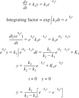
A.3.A First-Order Ordinary Differential Equation

See www.ucl.ac.uk/Mathematics/geomath/level2/deqn/de8.html and DVD-ROM Appendix K.

A-16

Using the integrating , the solution is

A-17

Where K₁ is a constant of integration.

Example A–1. Integrating Factor for Series Reactions

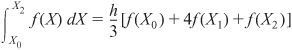
A.4 Numerical Evaluation of Integrals

In this section, we discuss techniques for numerically evaluating integrals for solving first-order differential equations.

1. Trapezoidal rule (two-point) (Figure A.2). This method is one of the simplest and most approximate, as it uses the integrand evaluated at the limits of integration to evaluate the integral:
   

   A-18

   

   when h = X₁ – X₀.

   Figure A.2. Trapezoidal rule illustration.

   

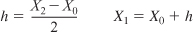
2. Simpson’s one-third rule (three-point) (Figure A.3). A more accurate evaluation of the integral can be found with the application of Simpson’s rule:
   

   A-19

   

   where

   

   Methods to solve in Chapters 2, 5, 11 and 12.

   Figure A.3. Simpson’s three-point rule illustration.

   

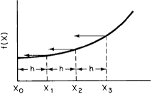
3. Simpson’s three-eighths rule (four-point) (Figure A.4). An improved version of Simpson’s one-third rule can be made by applying Simpson’s three-eighths rule:
   

   A-20

   

   where

   

   Figure A.4. Simpson’s four-point rule illustration.

   

4. Five-point quadrature formula.
   

   A-21

   

   where

5. For N + 1 points, where (N/3) is an integer,
   

   A-22

   

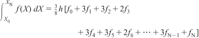
   where

6. For N + 1 points, where N is even,
   

   A-23

   

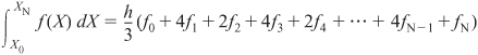
   where

These formulas are useful in illustrating how the reaction engineering integrals and coupled ODEs [ordinary differential equation(s)] can be solved and also when there is an ODE solver power failure or some other malfunction.