
Model Discrimination
One can also determine which model or equation best fits the experimental data by comparing the sums of the squares for each model and then choosing the equation with a smaller sum of squares and/or carrying out an F-test. Alternatively, we can compare the residual plots for each model. These plots show the error associated with each data point, and one looks to see if the error is randomly distributed or if there is a trend in the error. When the error is randomly distributed, this is an additional indication that the correct rate law has been chosen. An example of model discrimination using nonlinear regression is given on the DVD-ROM in Chapter 10 of the Summary Notes.
![]()
7.6 Reaction Rate Data from Differential Reactors
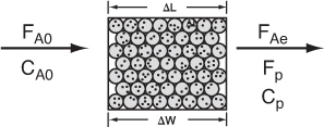
Data acquisition using the method of initial rates and a differential reactor is similar in that the rate of reaction is determined for a specified number of predetermined initial or entering reactant concentrations. A differential reactor (PBR) is normally used to determine the rate of reaction as a function of either concentration or partial pressure. It consists of a tube containing a very small amount of catalyst, usually arranged in the form of a thin wafer or disk. A typical arrangement is shown schematically in Figure 7-7. The criterion for a reactor being differential is that the conversion of the reactants in the bed is extremely small, as is the change in temperature and reactant concentration through the bed. As a result, the reactant concentration through the reactor is essentially constant and approximately equal to the inlet concentration. That is, the reactor is considered to be gradientless,3 and the reaction rate is considered spatially uniform within the bed.
Figure 7-7. Differential reactor.

The differential reactor is relatively easy to construct at a low cost. Owing to the low conversion achieved in this reactor, the heat release per unit volume will be small (or can be made small by diluting the bed with inert solids) so that the reactor operates essentially in an isothermal manner. When operating this reactor, precautions must be taken so that the reactant gas or liquid does not bypass or channel through the packed catalyst, but instead flows uniformly across the catalyst. If the catalyst under investigation decays rapidly, the differential reactor is not a good choice because the reaction rate parameters at the start of a run will be different from those at the end of the run. In some cases, sampling and analysis of the product stream may be difficult for small conversions in multicomponent systems.
Figure 7-8. Differential catalyst bed.
A → P
the volumetric flow rate through the catalyst bed is monitored, as are the entering and exiting concentrations (Figure 7-9). Therefore, if the weight of catalyst, ΔW, is known, the rate of reaction per unit mass of catalyst, ![]() , can be calculated. Since the differential reactor is assumed to be gradientless, the design equation will be similar to the CSTR design equation. A steady-state mole balance on reactant A gives
, can be calculated. Since the differential reactor is assumed to be gradientless, the design equation will be similar to the CSTR design equation. A steady-state mole balance on reactant A gives

The subscript e refers to the exit of the reactor. Solving for ![]() , we have
, we have
![]()
The mole balance equation can also be written in terms of concentration

or in terms of conversion or product flow rate FP:

The term FA0X gives the rate of formation of product, FP, when the stoichiometric coefficients of A and of P are identical. Adjustments to Equation (7-22) must be made when this is not the case.
For constant volumetric flow, Equation (7-22) reduces to
![]()
Consequently, we see that the reaction rate, ![]() , can be determined by measuring the product concentration, CP.
, can be determined by measuring the product concentration, CP.
By using very little catalyst and large volumetric flow rates, the concentration difference, (CA0 – CAe), can be made quite small. The rate of reaction determined from Equation (7-23) can be obtained as a function of the reactant concentration in the catalyst bed, CAb:
![]()
by varying the inlet concentration. One approximation of the concentration of A within the bed, CAb, would be the arithmetic mean of the inlet and outlet concentrations:
![]()
However, since very little reaction takes place within the bed, the bed concentration is essentially equal to the inlet concentration,
CAb ≈ CA0
so ![]() is a function of CA0:
is a function of CA0:
![]()
As with the method of initial rates [see DVD PRS R7.1], various numerical and graphical techniques can be used to determine the appropriate algebraic equation for the rate law. When collecting data for fluid-solid reacting systems, care must be taken that we use high flow rates through the differential reactor and small catalyst particle sizes in order to avoid mass transfer limitations. If data show the reaction to be first order with a low activation energy, say 8 kcal/moles, one should suspect the data is being collected in the mass transfer limited regime. We will expand on mass transfer limitations and how to avoid them in Chapter 10 and in Chapters DVD 11 and DVD 12 on the DVD-ROM.

Example 7-4. Using a Differential Reactor to Obtain Catalytic Rate Data
The formation of methane from carbon monoxide and hydrogen using a nickel catalyst was studied by Pursley.4 The reaction
3H2 + CO → CH4 + H2O
was carried out at 500°F in a differential reactor where the effluent concentration of methane was measured. The raw data is shown in Table E7-4.1.
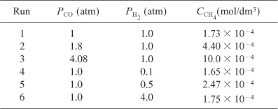
The exit volumetric flow rate from a differential packed bed containing 10 g of catalyst was maintained at 300 dm3/min for each run. The partial pressures of H2 and CO were determined at the entrance to the reactor, and the methane concentration was measured at the reactor exit.
a. Relate the rate of reaction to the exit methane concentration. The reaction rate law is assumed to be the product of a function of the partial pressure of CO and a function of the partial pressure of H2,
E7-4.1
![]()
b. Determine the rate law dependence on carbon monoxide, using the data generated in part (a). Assume that the functional dependence of ![]() on PCO is of the form
on PCO is of the form
E7-4.2
![]()
c. Determine the rate law dependence on H2. Generate a table of reaction rate as a function of partial pressures of carbon monoxide and hydrogen.
(a) In this example the product composition, rather than the reactant concentration, is being monitored. The term ![]() can be written in terms of the flow rate of methane from the reaction,
can be written in terms of the flow rate of methane from the reaction,
![]()
Substituting for FCH4 in terms of the volumetric flow rate and the concentration of methane gives
![]()
Since υ0, CCH4, and ΔW are known for each run, we can calculate the rate of reaction.
For run 1:
![]()
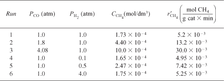
The rate for runs 2 through 6 can be calculated in a similar manner (Table E7-4.2).
Table E7-4.2. Raw and Calculated Data
(b) Determining the Rate Law Dependence in CO
For constant hydrogen concentration (Runs 1, 2, and 3), the rate law
![]()
can be written as
![]()
Taking the natural log of Equation (E7-5.4) gives us
![]()
We now plot ![]() versus ln PCO using runs 1, 2, and 3.
versus ln PCO using runs 1, 2, and 3.
(b) Runs 1, 2, and 3, for which the H2 concentration is constant, are plotted in Figure E7-4.1. We see from the Excel plot that α = 1.22. Had we included more points, we would have found that the reaction is essentially first order with α = 1, that is,
![]()
Figure E7-4.1. Reaction rate as a function of concentration.
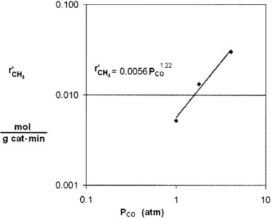
From the first three data points where the partial pressure of H2 is constant, we see the rate is linear in partial pressure of CO.
![]()
Now let’s look at the hydrogen dependence.
(c) Determining the Rate Law Dependence on H2
From Table E7-4.2 it appears that the dependence of ![]() on PH2 cannot be represented by a power law. Comparing run 4 with run 5 and then run 5 with run 6, we see that the reaction rate first increases with increasing partial pressure of hydrogen, and subsequently decreases with increasing PH2. That is, there appears to be a concentration of hydrogen at which the rate is maximum. One set of rate laws that is consistent with these observations is:
on PH2 cannot be represented by a power law. Comparing run 4 with run 5 and then run 5 with run 6, we see that the reaction rate first increases with increasing partial pressure of hydrogen, and subsequently decreases with increasing PH2. That is, there appears to be a concentration of hydrogen at which the rate is maximum. One set of rate laws that is consistent with these observations is:
- At low H2 concentrations where
 increases as PH2 increases, the rate law may be of the form

- At high H2 concentrations where decreases as PH2 increases,

We would like to find one rate law that is consistent with reaction rate data at both high and low hydrogen concentrations. After we have studied heterogeneous reactions in Chapter 10, we would recognize that Equations (E7-4.6) and (E7-4.7) can be combined into the form

We will see in Chapter 10 that this combination and similar rate laws which have reactant concentrations (or partial pressures) in the numerator and denominator are common in heterogeneous catalysis.
Let’s see if the resulting rate law (E7-4.8) is qualitatively consistent with the rate observed.
- For condition 1: At low PH2,
 and Equation (E7-4.8) reduces to

Equation (E7-4.9) is consistent with the trend in comparing runs 4 and 5.
- For condition 2: At high PH2,
 and Equation (E5-5.8) reduces to

where β2>β1. Equation (E7-4.10) is consistent with the trends in comparing runs 5 and 6.
Combining Equations (E7-4.8) and (E7-4.5)

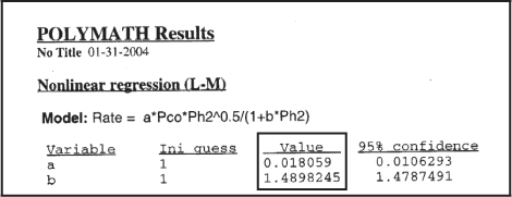
We now use the Polymath regression program to find the parameter values a, b, β1, and β2. The results are shown in Table E7-4.3.
Table E7-4.3. First Regression

Polymath regression tutorial is in the Chapter 5 Summary Notes.
The corresponding rate law is
![]()
We could use the rate law as given by Equation (E7-4.12) as is, but there are only six data points, and we should be concerned about extrapolating the rate law over a wider range of partial pressures. We could take more data, and/or we could carry out a theoretical analysis of the type discussed in Chapter 10 for heterogeneous reactions. If we assume hydrogen undergoes dissociative adsorption on the catalyst surface, we would expect a dependence on the partial pressure of hydrogen to be to the ½ power. Because 0.61 is close to 0.5, we are going to regress the data again, setting β1 = ½ and β2 = 1.0. The results are shown in Table E7-4.4.
Table E7-4.4. Second Regression
The rate law is now
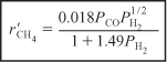
where ![]() is in (mol/gcat · s) and the partial pressures are in (atm).
is in (mol/gcat · s) and the partial pressures are in (atm).
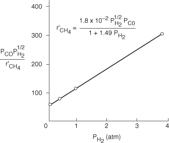
We could also have set β1 = ½ and β2 = 1.0 and rearranged Equation (E7-4.11) in the form
![]()
A plot of ![]() as a function of PH2 should be a straight line with an intercept of 1/a and a slope of b/a. From the plot in Figure E7-4.2, we see that the rate law is indeed consistent with the rate law data.
as a function of PH2 should be a straight line with an intercept of 1/a and a slope of b/a. From the plot in Figure E7-4.2, we see that the rate law is indeed consistent with the rate law data.
Figure E7-4.2. Linearized plot of data.
Analysis: The reaction rate data in this example were obtained at steady state, and as a result neither the integral method nor differential method of analysis can be used. One of the purposes of this example is to show how to reason out the form of the rate law and to then use regression to determine the rate law parameters. Once the parameters were obtained, we showed how to linearize the rate law [e.g., Equation (E7-4.13)] to generate a single plot of all the data, Figure (E7-4.2).
7.7 Experimental Planning
Four to six weeks in the lab can save you an hour in the library.
—Dr. G. C. Quarderer, Dow Chemical Co.
So far, this chapter has presented various methods of analyzing rate data. It is just as important to know in which circumstances to use each method as it is to know the mechanics of these methods. In PRS R7.5 on the DVD-ROM, we give a thumbnail sketch of a heuristic to plan experiments to generate the data necessary for reactor design. However, for a more thorough discussion, the reader is referred to the books and articles by Box and Hunter.5

Summary
- Integral method
a. Guess the reaction order and integrate the mole balance equation.
b. Calculate the resulting function of concentration for the data and plot it as a function of time. If the resulting plot is linear, you have probably guessed the correct reaction order.
c. If the plot is not linear, guess another order and repeat the procedure.
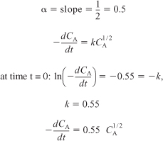
- Differential method for constant-volume systems

a. Plot –ΔCA/Δt as a function of t.
b. Determine –dCA/dt from this plot.
c. Take the ln of both sides of (S7-1) to get
S7-2

Plot ln (–dCA/dt) versus lnCA. The slope will be the reaction order α. We could use finite-difference formulas or software packages to evaluate (–dCA/dt) as a function of time and concentration.
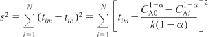
- Nonlinear regression: Search for the parameters of the rate law that will minimize the sum of the squares of the difference between the measured rate of reaction and the rate of reaction calculated from the parameter values chosen. For N experimental runs and K parameters to be determined, use Polymath.

Caution: Be sure to avoid a false minimum in σ2 by varying your initial guess.
- Modeling the differential reactor:
The rate of reaction is calculated from the equation

In calculating the reaction order, α,

the concentration of A is evaluated either at the entrance conditions or at a mean value between CA0 and CAe.
However, power law models such as

are not the best way to describe heterogeneous reaction rate laws. Typically, they take the form

or similar, with the reactant partial pressures in the numerator and denominator of the rate law.
DVD-ROM Material
• Learning Resources
- Summary Notes

- Interactive Computer Games

A. Ecology

B. Reactor Lab (www.SimzLab.com). See Reactor Lab Chapter 7 and P7-3B.
- Solved Problems
A. Example: Differential Method of Analysis of Pressure-Time Data
B. Example: Integral Method of Analysis of Pressure-Time Data
C. Example: Oxygenating Blood

• Living Example Problems
- Example 7-3 Use of Regression to Find the Rate Law Parameters

• FAQ [Frequently Asked Questions]—In Updates/FAQ icon section
• Professional Reference Shelf
R7.1 Method of Initial Rates
R7.2 Method of Half Lives
R7.3 Least Squares Analysis of the Linearized Rate Law
The DVD-ROM describes how the rate law
![]()
ln(–rA) = ln k + α ln CA + β ln CB
and put in the form
Y = a0 + αX1 + βX2
and used to solve for α, β, and k. The etching of a semiconductor, MnO2, is used as an example to illustrate this technique.
R7.4 A Discussion of Weighted Least Squares For the case when the error in measurement is not constant, we must use a weighted least squares analysis.
R7.5 Experimental Planning
A. Why perform the experiment?
B. Are you choosing the correct parameters?
C. What is the range of your experimental variables?
D. Can you repeat the measurement? (Precision)
E. Milk your data for all it’s worth.
F. We don’t believe an experiment until it’s proven by theory.
G. Tell someone about your result.
R7.6
Evaluation or Laboratory Reactors
Table 7-2. Summary of Reactor Ratings:* Gas–Liquid, Powdered Catalyst, Decaying Catalyst System†

Questions and Problems
The subscript to each of the problem numbers indicates the level of difficulty: A, least difficult; D, most difficult.
![]()

a.
Listen to the audios ![]() on the DVD-ROM and pick one and say why it could be eliminated.
on the DVD-ROM and pick one and say why it could be eliminated.
b.
Create an original problem based on Chapter 7 material.
c.
Design an experiment for the undergraduate laboratory that demonstrates the principles of chemical reaction engineering and will cost less than $500 in purchased parts to build. (From 1998 AIChE National Student Chapter Competition). Rules are provided on the DVD-ROM.
d.
K-12 Experiment. Plant a number of seeds in different pots (corn works well). The plant and soil of each pot will be subjected to different conditions. Measure the height of the plant as a function of time and fertilizer concentration. Other variables might include lighting, pH, and room temperature. (Great grade school or high school science project.)
![]()
a. Revisit Example 7-1. What is the error in assuming CB constant and what limits can you put on the calculated value of k? (I.e., k = 0.24 ±?).
b. Revisit Example 7-3. Explain why the regression was carried out twice to find k′ and k.
c. Revisit Example 7-4. Regress the data to fit the rate law
![]()
What is the difference in the correlation and sums-of-squares compared with those given in Example 7-4? Why was it necessary to regress the data twice, once to obtain Table E7-4.3 and once to obtain Table E7-4.4?
Load the Interactive Computer Game (ICG) from the DVD-ROM. Play the game and then record your performance number for the module which indicates your mastering of the material. Your professor has the key to decode your performance number.
ICM Ecology Performance # ________________.
Go to Professor Herz’s Reactor Lab on the DVD-ROM or on the Web at www.SimzLab.com. Do (a) one quiz, or (b) two quizzes from Division 1. When you first enter a lab, you see all input values and can vary them. In a lab, click on the Quiz button in the navigation bar to enter the quiz for that lab. In a quiz, you cannot see some of the input values: you need to find those with “???” hiding the values. In the quiz, perform experiments and analyze your data in order to determine the unknown values. See the bottom of the Example Quiz page at www.SimzLab.com for equations that relate E and k. Click on the “???” next to an input and supply your value. Your answer will be accepted if it is within ±20% of the correct value. Scoring is done with imaginary dollars to emphasize that you should design your experimental study rather than do random experiments. Each time you enter a quiz, new unknown values are assigned. To reenter an unfinished quiz at the same stage you left, click the [i] info button in the Directory for instructions. Turn in copies of your data, your analysis work, and the Budget Report.

When arterial blood enters a tissue capillary, it exchanges oxygen and carbon dioxide with its environment, as shown in this diagram.
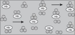
The kinetics of this deoxygenation of hemoglobin in blood was studied with the aid of a tubular reactor by Nakamura and Staub [J. Physiol., 173, 161].
![]()
Although this is a reversible reaction, measurements were made in the initial phases of the decomposition so that the reverse reaction could be neglected. Consider a system similar to the one used by Nakamura and Staub: the solution enters a tubular reactor (0.158 cm in diameter) that has oxygen electrodes placed at 5-cm intervals down the tube. The solution flow rate into the reactor is 19.6 cm3/s with CA0 = 2.33 × 10⁻⁶ mol/cm3.
![]()
a. Using the method of differential analysis of rate data, determine the reaction order and the forward specific reaction rate constant k1 for the deoxygenation of hemoglobin.
b. Repeat using regression.
The liquid-phase irreversible reaction
A → B + C
is carried out in a CSTR. To learn the rate law, the volumetric flow rate, υ0, (hence τ = V/υ0) is varied and the effluent concentrations of species A are recorded as a function of the space time τ. Pure A enters the reactor at a concentration of 2 mol/dm3. Steady-state conditions exist when the measurements are recorded.
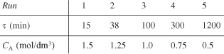
a. Determine the reaction order and specific reaction rate constant.
b. If you were to repeat this experiment to determine the kinetics, what would you do differently? Would you run at a higher, lower, or the same temperature? If you were to take more data, where would you place the measurements (e.g., τ)?
c. It is believed that the technician may have made a dilution factor-of-10 error in one of the concentration measurements. What do you think? How do your answers compare using regression (Polymath or other software) with those obtained by graphical methods?
Note: All measurements were taken at steady-state conditions.
The reaction
A → B + C
was carried out in a constant-volume batch reactor where the following concentration measurements were recorded as a function of time.
![]()
a. Use nonlinear least squares (i.e., regression) and one other method to determine the reaction order, α, and the specific reaction rate, k.
b. If you were to take more data, where would you place the points? Why?
c. If you were to repeat this experiment to determine the kinetics, what would you do differently? Would you run at a higher, lower, or the same temperature? Take different data points? Explain.
d. It is believed that the technician made a dilution error in the concentration measured at 60 min. What do you think? How do your answers compare using regression (Polymath or other software) with those obtained by graphical methods?
The liquid-phase reaction of methanol and triphenyl takes place in a batch reactor at 25°C
![]()
For an equal molar feed, the following concentration–time data was obtained for methanol:
![]()
The following concentration-time data were obtained for an initial methanol concentration 0.01 mol/dm3 and an initial triphenyl of 1.0 mol/dm3:
![]()
a. Determine the rate law and rate law parameters.
b. If you were to take more data points, what would be the reasonable settings (e.g., CA0, CB0)? Why?
The following data were reported [C. N. Hinshelwood and P. J. Ackey, Proc. R. Soc. (Lond)., A115, 215] for a gas-phase constant-volume decomposition of dimethyl ether at 504°C in a batch reactor. Initially, only (CH3)2O was present.
![]()
a. Why do you think the total pressure measurement at t = 0 is missing? Can you estimate it?
b. Assuming that the reaction
(CH3)2O → CH4 + H2 + CO
is irreversible and goes virtually to completion, determine the reaction order and specific reaction rate k.
c. What experimental conditions would you suggest if you were to obtain more data?
d. How would the data and your answers change if the reaction were run at a higher temperature? A lower temperature?
In order to study the photochemical decay of aqueous bromine in bright sunlight, a small quantity of liquid bromine was dissolved in water contained in a glass battery jar and placed in direct sunlight. The following data were obtained at 25°C:

![]()
a. Determine whether the reaction rate is zero, first, or second order in bromine, and calculate the reaction rate constant in units of your choice.
b. Assuming identical exposure conditions, calculate the required hourly rate of injection of bromine (in pounds per hour) into a sunlit body of water, 25,000 gal in volume, in order to maintain a sterilizing level of bromine of 1.0 ppm. [Ans.: 0.43 lb/h]
c. Apply one or more of the six ideas in Table P-3, page xiii to this problem. (Note: ppm = parts of bromine per million parts of brominated water by weight. In dilute aqueous solutions, 1 ppm ≡ 1 milligram per liter.) (From California Professional Engineers’ Exam.)
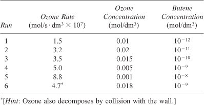
The reactions of ozone were studied in the presence of alkenes [R. Atkinson et al., Int. J. Chem. Kinet., 15(8), 721 (1983)]. The data in Table P7-10 are for one of the alkenes studied, cis-2-butene. The reaction was carried out isothermally at 297 K. Determine the rate law and the values of the rate law parameters.
Tests were run on a small experimental reactor used for decomposing nitrogen oxides in an automobile exhaust stream. In one series of tests, a nitrogen stream containing various concentrations of NO2 was fed to a reactor, and the kinetic data obtained are shown in Figure P7-11A. Each point represents one
Figure . Figure P7-11A Auto exhaust data.
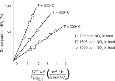
complete run. The reactor operates essentially as an isothermal backmix reactor (CSTR). What can you deduce about the apparent order of the reaction over the temperature range studied?
The plot gives the fractional decomposition of NO2 fed versus the ratio of reactor volume V (in cm3) to the NO2 feed rate, FNO2,0 (g mol/h), at different feed concentrations of NO2 (in parts per million by weight).
Microelectronic devices are formed by first forming SiO2 on a silicon wafer by chemical vapor deposition (Figure P7-12B). This procedure is followed by coating the SiO2 with a polymer called a photoresist. The pattern of the electronic circuit is then placed on the polymer and the sample is irradiated with ultraviolet light. If the polymer is a positive photoresist, the sections that were irradiated will dissolve in the appropriate solvent, and those sections not irradiated will protect the SiO2 from further treatment. The wafer is then exposed to strong acids, such as HF, which etch (i.e., dissolve) the exposed SiO2. It is extremely important to know the kinetics of the reaction, so that the proper depth of the channel can be achieved. The dissolution reaction is
SiO2 + 6HF → H2SiF6 + 2H2O
From the following initial rate data, determine the rate law.
![]()
Figure . Figure P7-12B Semiconductor etching.

A total of 1000 thin wafer chips are to be placed in 0.5 dm3 of 20% HF. If a spiral channel 10 μm wide and 10 m in length were to be etched to a depth of 50 μm on both sides of each wafer, how long should the chips be left in the solution? Assume that the solution is well mixed.
The thermal decomposition of isopropyl isocyanate was studied in a differential packed-bed reactor. From the data in Table P7-13C, determine the reaction rate law parameters.


• Additional Homework Problems are on the DVD-ROM
New Problems on the Web CDP7-New
CDP7-New
From time to time new problems relating Chapter 7 material to everyday interests or emerging technologies will be placed on the Web. Solutions to these problems can be obtained by emailing the author. Also, one can go to the Web site, www.rowan.edu/greenengineering, and work the home problem specific to this chapter.

Supplementary Reading
- A wide variety of techniques for measuring the concentrations of the reacting species may be found in
BURGESS, THORNTON W., Mr. Toad and Danny the Meadow Mouse Take a Walk. New York: Dover Publications, Inc., 1915.
FOGLER, H. SCOTT and STEVEN E. LEBLANC, Strategies for Creative Problem Solving. Englewood Cliffs, NJ: Prentice Hall, 1995.
KARRASS, CHESTER L., In Business As in Life, You Don’t Get What You Deserve, You Get What You Negotiate. Hill, CA: Stanford Street Press, 1996.
ROBINSON, J. W., Undergraduate Instrumental Analysis, 5th ed. New York: Marcel Dekker, 1995.
SKOOG, DOUGLAS A., F. JAMES HOLLER, and TIMOTHY A. NIEMAN, Principles of Instrumental Analysis, 5th ed. Philadelphia: Saunders College Publishers, Harcourt Brace College Publishers, 1998.
- The design of laboratory catalytic reactors for obtaining rate data is presented in
RASE, H. F., Chemical Reactor Design for Process Plants, Vol. 1. New York: Wiley, 1983, Chap. 5.
- The sequential design of experiments and parameter estimation is covered in
BOX, G. E. P., W. G. HUNTER, and J. S. HUNTER, Statistics for Experimenters: An Introduction to Design, Data Analysis, and Model Building. New York: Wiley, 1978.