
Chapter 7. Collection and Analysis of Rate Data
You can observe a lot just by watching.
—Yogi Berra, New York Yankees
7.1 The Algorithm for Data Analysis
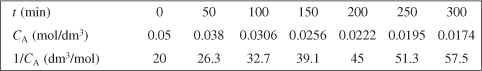
For batch systems, the usual procedure is to collect concentration-time data, which we then use to determine the rate law. Table 7-1 gives the seven-step procedure we will emphasize in analyzing reaction engineering data.
Data for homogeneous reactions is most often obtained in a batch reactor. After postulating a rate law in Step 1 and combining it with a mole balance in Step 2, we next use any or all of the methods in Step 5 to process the data and arrive at the reaction orders and specific reaction rate constants.
Analysis of heterogeneous reactions is shown in Step 6. For gas–solid heterogeneous reactions, we need to have an understanding of the reaction and possible mechanisms in order to postulate the rate law in Step 6B. After studying Chapter 10 on heterogeneous reactions, one will be able to postulate different rate laws and then use Polymath nonlinear regression to choose the “best” rate law and reaction rate law parameters.
The procedure we should use to delineate the rate law and rate law parameters is given in Table 7-1.
Table 7-1. Steps in Analyzing Rate Data
- Postulate a rate law.
A. Power law models for homogeneous reactions
B. Langmuir-Hinshelwood models for heterogeneous reactions
- Select reactor type and corresponding mole balance.
A. If batch reactor (Section 7.2), use mole balance on Reactant A
TE7-1.1

B. If differential PBR (Section 7.6), use mole balance on Product P (A → P)
TE7-1.2
- Process your data in terms of the measured variable (e.g., NA, CA, or PA). If necessary, rewrite your mole balance in terms of the measured variable (e.g., PA).
- Look for simplifications. For example, if one of the reactants is in excess, assume its concentration is constant. If the gas phase mole fraction of reactant A is small, set ε ≈ 0.
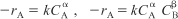
- For a batch reactor, calculate –rA as a function of concentration CA to determine the reaction order.
A. Differential analysis (Section 7-4)
Combine the mole balance (TE7-1.1) and power law model (TE7-1.3).
TE7-1.3

TE7-1.4

and then take the natural log.
TE7-1.5
- Find
 from CA versus t data by either the
a. Graphical differential
b. Finite differential method
c. Polynomial fit
- Either plot
 versus ln CA to find reaction order α, which is the slope of the line fit to the data or
 - Use regression to find α and k simultaneously.
B. Integral method (Section 7-3)
For
 , the combined mole balance and rate law is
Guess α and integrate Equation (TE7-1.4). Rearrange your equation to obtain the appropriate function of CA, which when plotted as a function of time should be linear. If it is linear, then the guessed value of α is correct and the slope is the specific reaction rate, k. If it is not linear, guess again for α. If you guess α = 0, 1, and 2 and none of these orders fit the data, proceed to nonlinear regression.
C. Nonlinear regression (Polymath) (Section 7-5):
Integrate Equation (TE7-1.4) to obtain

Use Polymath regression to find α and k. A Polymath tutorial on regression with screen shots is shown in the Chapter 7 Summary Notes on the DVD-ROM and Web.
- Find
- For differential PBR, calculate
 as a function of CA or PA (Section 7.6)
A. Calculate
 as a function of reactant concentration, CA or partial pressure PA.
B. Choose a model (see Chapter 10), e.g.,
C. Use nonlinear regression to find the best model and model parameters. See example on the DVD-ROM Summary Notes for Chapter 10, using data from heterogeneous catalysis.
- Analyze your rate law model for “goodness of fit.” Calculate a correlation coefficient.

7.2 Determining the Reaction Order for Each of Two Reactants Using the Method of Excess
Batch reactors are used primarily to determine rate law parameters for homogeneous reactions. This determination is usually achieved by measuring concentration as a function of time and then using either the differential, integral, or nonlinear regression method of data analysis to determine the reaction order, α, and specific reaction rate constant, k. If some reaction parameter other than concentration is monitored, such as pressure, the mole balance must be rewritten in terms of the measured variable (e.g., pressure, as shown in the example in Solved Problems on the DVD-ROM).
When a reaction is irreversible, it is possible in many cases to determine the reaction order α and the specific rate constant by either nonlinear regression or by numerically differentiating concentration versus time data. This latter method is most applicable when reaction conditions are such that the rate is essentially a function of the concentration of only one reactant; for example, if, for the decomposition reaction,
A → Products
![]()
then the differential method may be used.
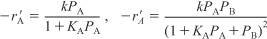
However, by utilizing the method of excess, it is also possible to determine the relationship between –rA and the concentration of other reactants. That is, for the irreversible reaction
A + B → Products
with the rate law
![]()
where α and β are both unknown, the reaction could first be run in an excess of B so that CB remains essentially unchanged during the course of the reaction (i.e., CB ≈ CB0) and
![]()
where
![]()
After determining α, the reaction is carried out in an excess of A, for which the rate law is approximated as
![]()
where ![]()
Once α and β are determined, kA can be calculated from the measurement of –rA at known concentrations of A and B:
![]()
Both α and β can be determined by using the method of excess, coupled with a differential analysis of data for batch systems.
7.3 Integral Method
This method is the quickest method to use to determine the rate law if the order turns out to zero, first, or second order. In the integral method, we guess the reaction order, α, in the combined batch reactor mole balance and rate law equation
![]()
and integrate the differential equation to obtain the concentration as a function of time. If the order we assume is correct, the appropriate plot (determined from this integration) of the concentration–time data should be linear. The integral method is used most often when the reaction order is known and it is desired to evaluate the specific reaction rate constant at different temperatures to determine the activation energy.
In the integral method of analysis of rate data, we are looking for the appropriate function of concentration corresponding to a particular rate law that is linear with time. You should be thoroughly familiar with the methods of obtaining these linear plots for reactions of zero, first, and second order.
For the reaction
A→Products
carried out in a constant-volume batch reactor, the mole balance is
![]()
It is important to know how to generate linear plots of functions of CA versus t for zero-, first-, and second-order reactions.
For a zero-order reaction, rA = –k, and the combined rate law and mole balance is
![]()
Integrating with CA = CA0 at t = 0, we have
![]()
A plot of the concentration of A as a function of time will be linear (Figure 7-1) with slope (–k) for a zero-order reaction carried out in a constant-volume batch reactor.
Figure 7-1. Zero-order reaction.

If the reaction is first order (Figure 7-2), integration of the combined mole balance and the rate law
![]()
with the limit CA = CA0 at t = 0 gives

Figure 7-2. First-order reaction.
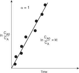
Consequently, we see that the slope of a plot of [ln(CA0/CA)] as a function of time is linear with slope k.
If the reaction is second order (Figure 7-3), then
![]()
Figure 7-3. Second-order reaction.

Integrating, with CA = CA0 initially, yields
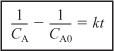
We see that for a second-order reaction a plot of (1/CA) as a function of time should be linear with slope k.
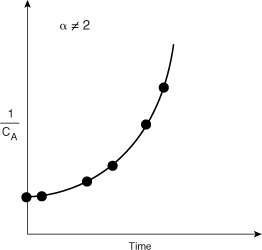
In Figures 7-1, 7-2, and 7-3, we saw that when we plotted the appropriate function of concentration (i.e., CA, ln CA, or 1/CA) versus time, the plots were linear, and we concluded that the reactions were zero, first, or second order, respectively. However, if the plots of concentration data versus time had turned out not to be linear, such as shown in Figure 7-4, we would say that the proposed reaction order did not fit the data. In the case of Figure 7-4, we would conclude that the reaction is not second order.
Figure 7-4. Plot of reciprocal concentration as a function of time.
It is important to restate that, given a reaction rate law, you should be able to quickly choose the appropriate function of concentration or conversion that yields a straight line when plotted against time or space time. The goodness-of-fit of such a line may be assessed statistically be calculating the linear correlation coefficient, r2, which should be as close to 1 as possible. The value of r2 is given in the output of Polymath’s non-linear regression.
Example 7-1. Integral Method of CRE Data Analysis
Trityl (A) + Methanol (B) → Products
was carried out in a batch reactor at 25°C in a solution of benzene and pyridine in an excess of methanol ![]() . Pyridine reacts with HCl, which then precipitates as pyridine hydro-chloride thereby making the reaction irreversible. The reaction is first order in methanol. The concentration of triphenyl methyl chloride (A) was measured as a function of time and is shown below
. Pyridine reacts with HCl, which then precipitates as pyridine hydro-chloride thereby making the reaction irreversible. The reaction is first order in methanol. The concentration of triphenyl methyl chloride (A) was measured as a function of time and is shown below
![]()
Use the integral method to confirm that the reaction is second order with regard to triphenyl methyl chloride
We use the power law model, Equation (7-2), along with information from the problem statement that the reaction is first order in methanol, (B), i.e., β = 1 to obtain
![]()
Excess methanol: The initial concentration of methanol (B) is 10 times that of trityl (A), so even if all A were consumed, 90% of B remains. Consequently, we will take the concentration of B as a constant and combine it with k to form
![]()
where k′ is the pseudo rate constant k′ = kCB0 and k is the true rate constant. Substituting α = 2 and combining with the mole balance on a batch reactor, we obtain
![]()
Integrating with CA = CA0 at t = 0
![]()
Rearranging
![]()
We see that if the reaction is indeed second order then a plot of (1/CA) versus t should be linear. The data in Table E7-1.1 will be used to construct Table E7-1.2.
In a graphical solution, the data in Table E7-1.2 can be used to construct a plot of 1/CA as a function of t, which will yield the specific reaction rate k′. This plot is shown in Figure E7-1.1. Again, one could use Excel or Polymath to find k′ from the data in Table E7-1.2. The slope of the line is the specific reaction rate k′
Figure E7-1.1. Plot of the reciprocal of CA versus t for a second-order reaction.

We see from the Excel analysis and plot that the slope of the line is 0.12 dm3/mol · min.
![]()
We now use Equation (E7-1.6), along with the initial concentration of methanol, to find the true rate constant, k.
![]()
The rate law is
![]()
We note in passing that the integral method tends to smooth the data.
Analysis: In this example the reaction orders are known so that the integral method can be used to (1) verify the reaction is second order in trityl and (2) to find the specific pseudo reaction rate k′ = kCB0 for the case of excess methanol (B). Knowing k′ and CB0, we can then find the true rate constant k.
7.4 Differential Method of Analysis
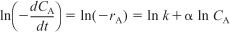
To outline the procedure used in the differential method of analysis, we consider a reaction carried out isothermally in a constant-volume batch reactor and the concentration of A, recorded as a function of time. By combining the mole balance with the rate law given by Equation (7-1), we obtain
![]()
After taking the natural logarithm of both sides of Equation (5-6),
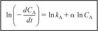
observe that the slope of a plot of [ln(–dCA/dt)] as a function of (ln CA) is the reaction order, α (Figure 7-5).
Figure 7-5. Differential method to determine reaction order.
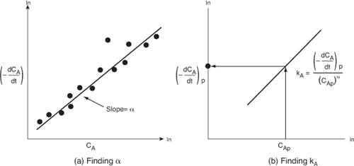
Figure 7-5(a) shows a plot of [–(dCA/dt)] versus [CA] on log-log paper (or use Excel to make the plot) where the slope is equal to the reaction order α. The specific reaction rate, kA, can be found by first choosing a concentration in the plot, say CAp, and then finding the corresponding value of [–(dCA/dt)p] on the line, as shown in Figure 7-5(b). The concentration chosen, CAp, to find the derivative at CAp, need not be a data point. After raising CAp to the α power, we divide it into [–(dCA/dt)p] to determine kA:
![]()
To obtain the derivative (–dCA/dt) used in this plot, we must differentiate the concentration-time data either numerically or graphically. Three methods to determine the derivative from data giving the concentration as a function of time. These methods are:
• Graphical differentiation
• Numerical differentiation formulas
• Differentiation of a polynomial fit to the data
We shall only discuss the graphical method.