
2.3.3 Packed-Bed Reactor (PBR)
Packed-bed reactors are tubular reactors filled with catalyst particles. In PBRs it is the weight of catalyst W that is important, rather than the reactor volume. The derivation of the differential and integral forms of the design equations for packed-bed reactors are analogous to those for a PFR [cf. Equations (2-15) and (2-16)]. That is, substituting Equation (2-12) for FA in Equation (1-15) gives
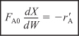
The differential form of the design equation [i.e., Equation (2-17)] must be used when analyzing reactors that have a pressure drop along the length of the reactor. We discuss pressure drop in packed-bed reactors in Chapter 5.
In the absence of pressure drop, i.e., ΔP = 0, we can integrate (2-17) with limits X = 0 at W = 0 and when W = W then X = X to obtain

Equation (2-18) can be used to determine the catalyst weight W (i.e., mass) necessary to achieve a conversion X when the total pressure remains constant.
2.4 Sizing Continuous-Flow Reactors
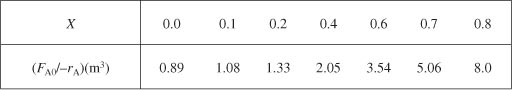
In this section, we are going to show how we can size CSTRs and PFRs (i.e., determine their reactor volumes) from knowledge of the rate of reaction, –rA, as a function of conversion, X [i.e., –rA = f(X)]. The rate of disappearance of A, –rA, is almost always a function of the concentrations of the various species present (see Chapter 3). When only one reaction is occurring, each of the concentrations can be expressed as a function of the conversion X (see Chapter 4); consequently, –rA can be expressed as a function of X.
A particularly simple functional dependence, yet one that occurs often, is the first-order dependence
–rA = kCA = kCA0(1 – X)
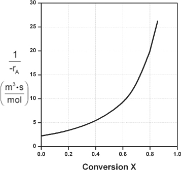
Here, k is the specific reaction rate and is a function only of temperature, and CA0 is the entering concentration of A. We note in Equations (2-13) and (2-16) that the reactor volume is a function of the reciprocal of –rA. For this first-order dependence, a plot of the reciprocal rate of reaction (1/–rA) as a function of conversion yields a curve similar to the one shown in Figure 2-1, where
Figure 2-1. Reciprocal rate as a function of conversion.
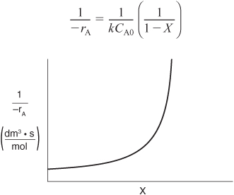
We can use Figure 2-1 to size CSTRs and PFRs for different entering flow rates. By sizing we mean either determine the reactor volume for a specified conversion or determine the conversion for a specified reactor volume. Before sizing flow reactors, let’s consider some insights. If a reaction is carried out isothermally, the rate is usually greatest at the start of the reaction when the concentration of reactant is greatest (i.e., when there is negligible conversion [X ≅ 0]). Hence, the reciprocal rate (1/–rA) will be small. Near the end of the reaction, when the reactant has been mostly used up and thus the concentration of A is small (i.e., the conversion is large), the reaction rate will be small. Consequently, the reciprocal rate (1/–rA) is large.
For all irreversible reactions of greater than zero order (see Chapter 3 for zero-order reactions), as we approach complete conversion where all the limiting reactant is used up, i.e., X = 1, the reciprocal rate approaches infinity as does the reactor volume, i.e.
As X → 1, –rA → 0, thus, ![]() therefore V → ∞
therefore V → ∞
Consequently, we see that an infinite reactor volume is necessary to reach complete conversion, X = 1.0.
For reversible reactions (e.g., A bhanu& B), the maximum conversion is the equilibrium conversion Xe. At equilibrium, the reaction rate is zero (rA ≡ 0). Therefore,
As X → Xe, –rA → 0, thus, ![]() and therefore V → ∞
and therefore V → ∞
and we see that an infinite reactor volume would also be necessary to obtain the exact equilibrium conversion, X = Xe. More on Xe in Chapter 4.
Examples
To illustrate the design of continuous flow reactors (i.e., CSTRs and PFRs), we consider the isothermal gas-phase isomerization
![]()
We are going to the laboratory to determine the rate of chemical reaction as a function of the conversion of reactant A. The laboratory measurements given in Table 2-1 show the chemical reaction rate as a function of conversion. The temperature was 500 K (440°F), the total pressure was 830 kPa (8.2 atm), and the initial charge to the reactor was pure A. The entering molar flow of A rate is FA0 = 0.4 mol/s.
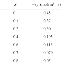
Recalling the CSTR and PFR design equations, (2-13) and (2-16), we see that the reactor volume varies directly with the molar flow rate FA0 and with the reciprocal of –rA, ![]() , e.g.,
, e.g., ![]() . Consequently, to size reactors, we first convert the raw data in Table 2-1, which gives –rA as a function of X first to
. Consequently, to size reactors, we first convert the raw data in Table 2-1, which gives –rA as a function of X first to ![]() as a function of X. Next, we multiply by the entering molar flow rate, FA0, to obtain
as a function of X. Next, we multiply by the entering molar flow rate, FA0, to obtain ![]() as a function of X as shown in Table 2-2 of the processed data for FA0 = 0.4 mol/s.
as a function of X as shown in Table 2-2 of the processed data for FA0 = 0.4 mol/s.

To size reactors for different entering molar flow rates, FA0, we would use rows 1 and 3 in Table 2-2 to construct the following figure:
However, for a given FA0, rather than use Figure 2-2A to size reactors, it is often more advantageous to plot ![]() as a function of X, which is called a Levenspiel plot. We are now going to carry out a number of examples where we have specified the flow rate FA0 at 0.4 mol A/s.
as a function of X, which is called a Levenspiel plot. We are now going to carry out a number of examples where we have specified the flow rate FA0 at 0.4 mol A/s.
Figure 2-2A. Processed data 1.
Plotting ![]() as a function of X using the data in Table 2-2 we obtain the plot shown in Figure 2-2B.
as a function of X using the data in Table 2-2 we obtain the plot shown in Figure 2-2B.
Figure 2-2B. Levenspiel plot of processed data 2.
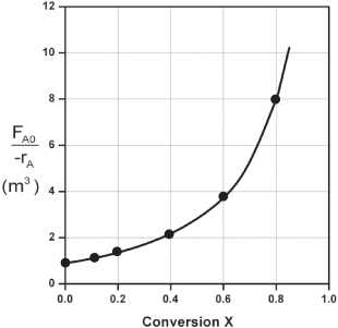
We are now going to use the Levenspiel plot of the processed data (Figure 2-2B) to size a CSTR and a PFR.
The reaction described by the data in Table 2-2
A → B
is to be carried out in a CSTR. Species A enters the reactor at a molar flow rate of ![]() , which is the flow rate used to construct Figure 2-2B.
, which is the flow rate used to construct Figure 2-2B.
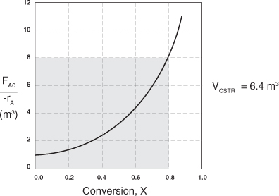
a. Using the data in either Table 2-2 or Figure 2-2B, calculate the volume necessary to achieve 80% conversion in a CSTR.
b. Shade the area in Figure 2-2B that would give the CSTR volume necessary to achieve 80% conversion.
a. Equation (2-13) gives the volume of a CSTR as a function of FA0, X, and –rA:
2-13
![]()
In a CSTR, the composition, temperature, and conversion of the effluent stream are identical to that of the fluid within the reactor, because perfect mixing is assumed. Therefore, we need to find the value of –rA (or reciprocal thereof) at X = 0.8. From either Table 2-2 or Figure 2-2A, we see that when X = 0.8, then
![]()
Substitution into Equation (2-13) for an entering molar flow rate, FA0, of 0.4 mol A/s and X = 0.8 gives
E2-1.1
b. Shade the area in Figure 2-2B that yields the CSTR volume. Rearranging Equation (2-13) gives
2-13
![]()
In Figure E2-1.1, the volume is equal to the area of a rectangle with a height (FA0/–rA = 8 m3) and a base (X = 0.8). This rectangle is shaded in the figure.
E2-1.2
![]()
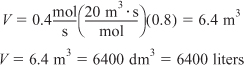
V = Levenspiel rectangle area = height × width
V = [8 m3][0.8] = 6.4 m3
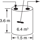
Figure E2-1.1. Levenspiel CSTR plot.
The CSTR volume necessary to achieve 80% conversion is 6.4 m3 when operated at 500 K, 830 kPa (8.2 atm), and with an entering molar flow rate of A of 0.4 mol/s. This volume corresponds to a reactor about 1.5 m in diameter and 3.6 m high. It’s a large CSTR, but this is a gas-phase reaction, and CSTRs are normally not used for gas-phase reactions. CSTRs are used primarily for liquid-phase reactions.
Analysis: Given the conversion, the rate of reaction as a function of conversion along with the molar flow of the species A, we saw how to calculate the volume of a CSTR. From the data and information given, we calculated the volume to be 6.4 m3 for 80% conversion. We showed how to carry out this calculation using the design equation (2-13) and also using a Levenspiel plot.
The reaction described by the data in Tables 2-1 and 2-2 is to be carried out in a PFR. The entering molar flow rate of A is again 0.4 mol/s.
a. First, use one of the integration formulas given in Appendix A.4 to determine the PFR reactor volume necessary to achieve 80% conversion.
b. Next, shade the area in Figure 2-2B that would give the PFR volume necessary to achieve 80% conversion.
c. Finally, make a qualitative sketch of the conversion, X, and the rate of reaction, –rA, down the length (volume) of the reactor.
We start by repeating rows (1) and (4) of Table 2-2 to produce the results shown in Table 2-3.
a. For the PFR, the differential form of the mole balance is
2-15
![]()
Rearranging and integrating gives
2-16
![]()
We shall use the five point quadrature formula [Equation (A-23)] given in Appendix A.4 to numerically evaluate Equation (2-16). The five-point formula with a final conversion of 0.8 gives four equal segments between X = 0 and X = 0.8 with a segment length of ![]() . The function inside the integral is evaluated at X = 0, X = 0.2, X = 0.4, X = 0.6, and X = 0.8.
. The function inside the integral is evaluated at X = 0, X = 0.2, X = 0.4, X = 0.6, and X = 0.8.
E2-2.1
![]()
Using values of [FA0/(–rA)] corresponding to the different conversions in Table 2-3 yields
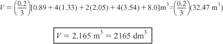
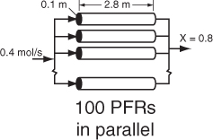
The PFR reactor volume necessary to achieve 80% conversion is 2165 dm3. This volume could result from a bank of 100 PFRs that are each 0.1 m in diameter with a length of 2.8 m (e.g., see margin figure or Figures 1-8(a) and (b)).
.b The integral in Equation (2-16) can also be evaluated from the area under the curve of a plot of (FA0/–rA) versus X.
![]()
= Area under the curve between X = 0 and X = 0.8 (see shaded area in Figure E2-2.1)
Figure E2-2.1. Levenspiel PFR plot.
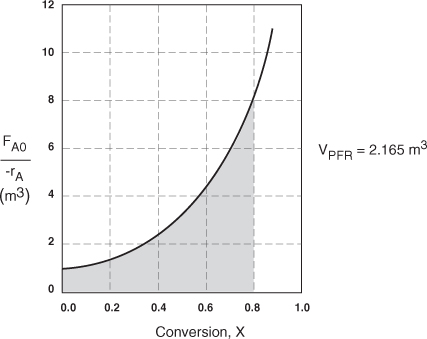
The area under the curve will give the tubular reactor volume necessary to achieve the specified conversion of A. For 80% conversion, the shaded area is roughly equal to 2165 dm3 (2.165 m3).
c. Sketch the profiles of –rA and X down the length of the reactor.
We know that as we proceed down the reactor, the conversion increases as more and more reactant is converted to product. Consequently, as the reactant is consumed, the concentration of reactant decreases, as does the rate of disappearance of A for isothermal reactions.
i. For X = 0.2, we calculate the corresponding reactor volume using Simpson’s rule [given in Appendix A.4 as Equation (A-21)] with increment ΔX = 0.1 and the data in rows 1 and 4 in Table 2-2,
E2-2.2
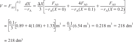
This volume (218 dm3) is the volume at which X = 0.2. From Table 2-3 we see the corresponding rate of reaction at X = 0.2 is ![]() .
.
Therefore at X = 0.2, then ![]() and V = 218 dm3.
and V = 218 dm3.
ii. For X = 0.4, we can again use Table 2-3 and Simpson’s rule with Δ X = 0.2 to find the reactor volume necessary for a conversion of 40%.
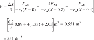
From Table 2-3 we see that at X = 0.4, ![]() and V = 551 dm3.
and V = 551 dm3.
We can continue in this manner to arrive at Table E2-2.1.
Table E2-2.1. Conversion and Reaction Rate Profiles
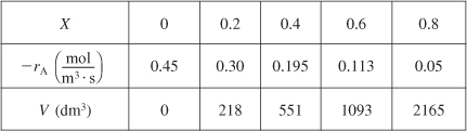
The data in Table E2-2.1 are plotted in Figures E2-2.2(a) and (b).
Figure E2-2.2(a). Conversion profile.
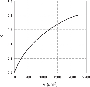
Figure E2-2.2(b). Reaction rate profile.
Analysis: One observes that the reaction rate, –rA, decreases as we move down the reactor while the conversion increases. These plots are typical for reactors operated isothermally.
Example 2-3. Comparing CSTR and PFR Sizes
Compare the volumes of a CSTR and a PFR required for the same conversion using the data in Figure 2-2B. Which reactor would require the smaller volume to achieve a conversion of 80%: a CSTR or a PFR? The entering molar flow rate and the feed conditions are the same in both cases.
We will again use the data in Table 2-3.

The CSTR volume was 6.4 m3 and the PFR volume was 2.165 m3. When we combine Figures E2-1.1 and E2-2.1 on the same graph, Figure 2-3.1(a), we see that the crosshatched area above the curve is the difference in the CSTR and PFR reactor volumes.
For isothermal reactions greater than zero order (see Chapter 3), the CSTR volume will always be greater than the PFR volume for the same conversion and reaction conditions (temperature, flow rate, etc.).
Figure E2-3.1(a). Comparison of CSTR and PFR reactor sizes for X = 0.8.
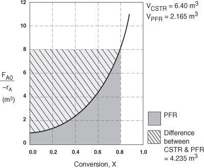
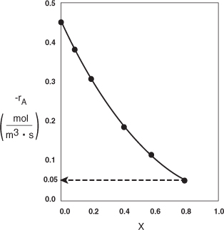
Analysis: We see that the reason the isothermal CSTR volume is usually greater than the PFR volume is that the CSTR is always operating at the lowest reaction rate (e.g., –rA = 0.05 mol/m3·s in Figure E2-3.1(b)). The PFR on the other hand starts at a high rate at the entrance and gradually decreases to the exit rate, thereby requiring less volume because the volume is inversely proportional to the rate. However, there are exceptions such as autocatalytic reactions, product-inhibited reactions, and nonisothermal exothermic reactions; these trends will not always be the case, as we will see in Chapters 9 and 11.
Figure E2-3.1(b). –rA as a function of X obtained from Table 2-2.1.
2.5 Reactors in Series
Many times, reactors are connected in series so that the exit stream of one reactor is the feed stream for another reactor. When this arrangement is used, it is often possible to speed calculations by defining conversion in terms of location at a point downstream rather than with respect to any single reactor. That is, the conversion X is the total number of moles of A that have reacted up to that point per mole of A fed to the first reactor.
For reactors in series
![]()
However, this definition can only be used when the feed stream only enters the first reactor in the series and there are no side streams either fed or withdrawn. The molar flow rate of A at point i is equal to the moles of A fed to the first reactor, minus all the moles of A reacted up to point i.
FAi = FA0 – FA0Xi

For the reactors shown in Figure 2-3, X1 at point i = 1 is the conversion achieved in the PFR, X2 at point i = 2 is the total conversion achieved at this point in the PFR and the CSTR, and X3 is the total conversion achieved by all three reactors.
Figure 2-3. Reactors in series.
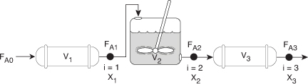
To demonstrate these ideas, let us consider three different schemes of reactors in series: two CSTRs, two PFRs, and then a combination of PFRs and CSTRs in series. To size these reactors, we shall use laboratory data that gives the reaction rate at different conversions.