
9.2.3 Michaelis–Menten Equation
Because the reaction of urea and urease is carried out in aqueous solution, water is, of course, in excess, and the concentration of water is therefore considered constant. Let
![]()
Dividing the numerator and denominator of Equation (9-24) by k1, we obtain a form of the Michaelis–Menten equation:
![]()
The parameter kcat is also referred to as the turnover number. It is the number of substrate molecules converted to product in a given time on a single-enzyme molecule when the enzyme is saturated with substrate (i.e., all the active sites on the enzyme are occupied, (S)>>KM). For example, the turnover number for the decomposition of hydrogen-peroxide, H2O2, by the enzyme catalase is 40 × 106 s–1. That is, 40 million molecules of H2O2 are decomposed every second on a single-enzyme molecule saturated with H2O2. The constant KM (mol/dm3) is called the Michaelis constant and for simple systems is a measure of the attraction of the enzyme for its substrate, so it’s also called the affinity constant. The Michaelis constant, KM, for the decomposition of H2O2 discussed earlier is 1.1 M, while that for chymotrypsin is 0.1 M.9
If, in addition, we let Vmax represent the maximum rate of reaction for a given total enzyme concentration,
Vmax = kcat(Et)
the Michaelis–Menten equation takes the familiar form
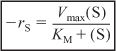
For a given enzyme concentration, a sketch of the rate of disappearance of the substrate is shown as a function of the substrate concentration in Figure 9-6.
Figure 9-6. Michaelis–Menten plot identifying the parameters Vmax and KM.

A plot of this type is sometimes called a Michaelis–Menten plot. At low substrate concentration, ![]() ,
,
![]()
and the reaction is apparent first order in the substrate concentration. At high substrate concentrations,
![]()
and the reaction is apparent zero order
–rS ≅ Vmax
What does KM represent? Consider the case when the substrate concentration is such that the reaction rate is equal to one-half the maximum rate,
![]()
then
![]()
Solving Equation (9-27) for the Michaelis constant yields
![]()
The Michaelis constant is equal to the substrate concentration at which the rate of reaction is equal to one-half the maximum rate. The larger the value of KM, the higher the substrate concentration necessary for the reaction rate to reach half of its maximum value.
The parameters Vmax and KM characterize the enzymatic reactions that are described by Michaelis–Menten kinetics. Vmax is dependent on total enzyme concentration, whereas KM is not.
Two enzymes may have the same values for kcat but have different reaction rates because of different values of KM. One way to compare the catalytic efficiencies of different enzymes is to compare their ratios kcat/KM. When this ratio approaches 108 to 109 (dm3/mol/s), the reaction rate approaches becoming diffusion-limited. That is, it takes a long time for the enzyme and substrate to find each other, but once they do they react immediately. We will discuss diffusion-limited reactions in PRS Chapters DVD11 and DVD12 on the DVD-ROM.
Example 9-2. Evaluation of Michaelis–Menten Parameters Vmax and KM
Determine the Michaelis–Menten parameters Vmax and KM for the reaction

The rate of reaction is given as a function of urea concentration in the table below, where (S) ≡ Curea.

Inverting Equation (9-26) gives us the Lineweaver–Burk equation
![]()
or
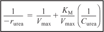
A plot of the reciprocal reaction rate versus the reciprocal urea concentration should be a straight line with an intercept (1/Vmax) and slope (KM/Vmax). This type of plot is called a Lineweaver–Burk plot. We shall use the data in Table E9-2.1 to make two plots. A plot of –rurea as a function of Curea using Equation (9-26) which is called a Michaelis–Menten plot and is shown in Figure E9-2.1(a). A plot of (1/–rurea) as a function (1/Curea), which is called a Lineweaver–Burk plot, is shown in Figure 9-2.1 (b).
Table E9-2.1. Raw and Processed Data


Michaelis–Menten Plot

Lineweaver–Burk Plot
Figure E9-2.1. (a) Michaelis–Menten plot; (b) Lineweaver–Burk plot.

The intercept on Figure E9-2.1(b) is 0.75, so
![]()
Therefore, the maximum rate of reaction is
Vmax = 1.33 kmol/m3·s = 1.33 mol/dm3·s
From the slope, which is 0.02 s, we can calculate the Michaelis constant, KM:

Substituting KM and Vmax into Equation (9-26) gives us
![]()
where Curea has units of (kmol/m3) and –rurea has units of (kmol/m3·s). Levine and LaCourse suggest that the total concentration of urease, (Et), corresponding to the value of Vmax above is approximately 5 g/dm3.
In addition to the Lineweaver–Burk plot, one can also use a Hanes–Woolf plot or an Eadie–Hofstee plot. Here S ≡ Curea, and –rS ≡ –rurea. Equation (9-26)
![]()
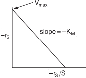
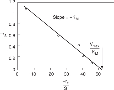
can be rearranged in the following forms. For the Eadie–Hofstee form,
![]()
For the Hanes–Woolf form, we can rearrange Equation (9-26) to
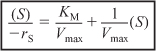

For the Eadie–Hofstee model we plot –rS as a function of [–rS/(S)] and for the Hanes–Woolf model, we plot [(S)/–rS] as a function of (S). The Eadie–Hofstee plot does not bias the points at low substrate concentrations, while the Hanes–Woolf plot gives a more accurate evaluation of Vmax. In Table E9-2.2, we add two columns to Table E9-2.1 to generate these plots (Curea ≡ S).
Table E9-2.2. Raw and Processed Data

Plotting the data in Table E9-2.2, we arrive at Figures E9-2.2 and E9-2.3.
Figure E9-2.2. Hanes–Woolf plot.
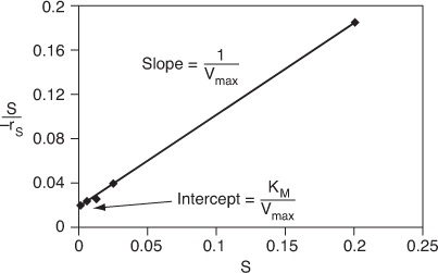
Figure E9-2.3. Eadie–Hofstee plot.
Equation (9-26) and Table E9-2.1 were used in the regression program of Polymath with the following results for Vmax and KM.
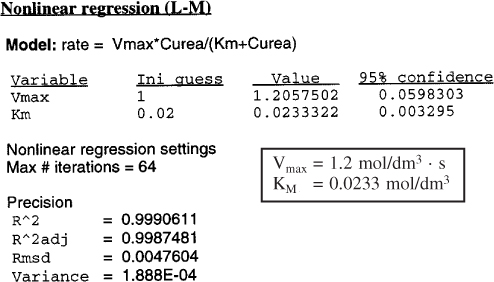
These values are within experimental error of those values of Vmax and Km determined graphically.
Analysis: This example demonstrated how to evaluate the parameters Vmax and KM in the Michaelis–Menten rate law from enzymatic reaction data. Two techniques were used: a Lineweaver–Burk plot and non-linear regression. It was also shown how the analysis could be carried out using Hanes–Woolf and Eadie–Hofstee plots.
The Product-Enzyme Complex
In many reactions the enzyme and product complex (E · P) is formed directly from the enzyme substrate complex (E · S) according to the sequence
![]()
Applying the PSSH, we obtain
![]()
which is often referred to as the Briggs–Haldane Equation [see P9-8B (a)] and the application of the PSSH to enzyme kinetics, often called the Briggs–Haldane approximation.