
Chapter 15. Ray Casting and Rasterization
15.1. Introduction
Previous chapters considered modeling and interacting with 2D and 3D scenes using an underlying renderer provided by WPF. Now we focus on writing our own physically based 3D renderer.
Rendering is integration. To compute an image, we need to compute how much light arrives at each pixel of the image sensor inside a virtual camera. Photons transport the light energy, so we need to simulate the physics of the photons in a scene. However, we can’t possibly simulate all of the photons, so we need to sample a few of them and generalize from those to estimate the integrated arriving light. Thus, one might also say that rendering is sampling. We’ll tie this integration notion of sampling to the alternative probability notion of sampling presently.
In this chapter, we look at two strategies for sampling the amount of light transported along a ray that arrives at the image plane. These strategies are called ray casting and rasterization. We’ll build software renderers using each of them. We’ll also build a third renderer using a hardware rasterization API. All three renderers can be used to sample the light transported to a point from a specific direction. A point and direction define a ray, so in graphics jargon, such sampling is typically referred to as “sampling along a ray,” or simply “sampling a ray.”
There are many interesting rays along which to sample transport, and the methods in this chapter generalize to all of them. However, here we focus specifically on sampling rays within a cone whose apex is at a point light source or a pinhole camera aperture. The techniques within these strategies can also be modified and combined in interesting ways. Thus, the essential idea of this chapter is that rather than facing a choice between distinct strategies, you stand to gain a set of tools that you can modify and apply to any rendering problem. We emphasize two aspects in the presentation: the principle of sampling as a mathematical tool and the practical details that arise in implementing real renderers.
Of course, we’ll take many chapters to resolve the theoretical and practical issues raised here. Since graphics is an active field, some issues will not be thoroughly resolved even by the end of the book. In the spirit of servicing both principles and practice, we present some ideas first with pseudocode and mathematics and then second in actual compilable code. Although minimal, that code follows reasonable software engineering practices, such as data abstraction, to stay true to the feel of a real renderer. If you create your own programs from these pieces (which you should) and add the minor elements that are left as exercises, then you will have three working renderers at the end of the chapter. Those will serve as a scalable code base for your implementation of other algorithms presented in this book.
The three renderers we build will be simple enough to let you quickly understand and implement them in one or two programming sessions each. By the end of the chapter, we’ll clean them up and generalize the designs. This generality will allow us to incorporate changes for representing complex scenes and the data structures necessary for scaling performance to render those scenes.
We assume that throughout the subsequent rendering chapters you are implementing each technique as an extension to one of the renderers that began in this chapter. As you do, we recommend that you adopt two good software engineering practices.
1. Make a copy of the renderer before changing it (this copy becomes the reference renderer).
2. Compare the image result after a change to the preceding, reference result.
Techniques that enhance performance should generally not reduce image quality. Techniques that enhance simulation accuracy should produce noticeable and measurable improvements. By comparing the “before” and “after” rendering performance and image quality, you can verify that your changes were implemented correctly.
Comparison begins right in this chapter. We’ll consider three rendering strategies here, but all should generate identical results. We’ll also generalize each strategy’s implementation once we’ve sketched it out. When debugging your own implementations of these, consider how incorrectly mismatched results between programs indicate potential underlying program errors. This is yet another instance of the Visual Debugging principle.
15.2. High-Level Design Overview
We start with a high-level design in this section. We’ll then pause to address the practical issues of our programming infrastructure before reducing that high-level design to the specific sampling strategies.
15.2.1. Scattering
Light that enters the camera and is measured arrives from points on surfaces in the scene that either scattered or emitted the light. Those points lie along the rays that we choose to sample for our measurement. Specifically, the points casting light into the camera are the intersections in the scene of rays, whose origins are points on the image plane, that passed through the camera’s aperture.
To keep things simple, we assume a pinhole camera with a virtual image plane in front of the center of projection, and an instantaneous exposure. This means that there will be no blur in the image due to defocus or motion. Of course, an image with a truly zero-area aperture and zero-time exposure would capture zero photons, so we take the common graphics approximation of estimating the result of a small aperture and exposure from the limiting case, which is conveniently possible in simulation, albeit not in reality.
We also assume that the virtual sensor pixels form a regular square grid and estimate the value that an individual pixel would measure using a single sample at the center of that pixel’s square footprint. Under these assumptions, our sampling rays are the ones with origins at the center of projection (i.e., the pinhole) and directions through each of the sensor-pixel centers.1
1. For the advanced reader, we acknowledge Alvy Ray Smith’s “a pixel is not a little square”—that is, no sample is useful without its reconstruction filter—but contend that Smith was so successful at clarifying this issue that today “sample” now is properly used to describe the point-sample data to which Smith referred, and “pixel” now is used to refer to a “little square area” of a display or sensor, whose value may be estimated from samples. We’ll generally use “sensor pixel” or “display pixel” to mean the physical entity and “pixel” for the rectangular area on the image plane.
Finally, to keep things simple we chose a coordinate frame in which the center of projection is at the origin and the camera is looking along the negative z-axis. We’ll also refer to the center of projection as the eye. See Section 15.3.3 for a formal description and Figure 15.1 for a diagram of this configuration.
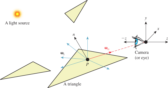
Figure 15.1: A specific surface location P that is visible to the camera, incident light at P from various directions {ωi}, and the exitant direction ωo toward the camera.
The light that arrived at a specific sensor pixel from a scene point P came from some direction. For example, the direction from the brightest light source in the scene provided a lot of light. But not all light arrived from the brightest source. There may have been other light sources in the scene that were dimmer. There was also probably a lot of light that previously scattered at other points and arrived at P indirectly. This tells us two things. First, we ultimately have to consider all possible directions from which light may have arrived at P to generate a correct image. Second, if we are willing to accept some sampling error, then we can select a finite number of discrete directions to sample. Furthermore, we can probably rank the importance of those directions, at least for lights, and choose a subset that is likely to minimize sampling error.
We don’t expect you to have perfect answers to these, but we want you to think about them now to help develop intuition for this problem: What kind of errors could arise from sampling a finite number of directions? What makes them errors? What might be good sampling strategies? How do the notions of expected value and variance from statistics apply here? What about statistical independence and bias?
Let’s start by considering all possible directions for incoming light in pseudocode and then return to the ranking of discrete directions when we later need to implement directional sampling concretely.
To consider the points and directions that affect the image, our program has to look something like Listing 15.1.
Listing 15.1: High-level rendering structure.
1 for each visible point P with direction ωo from it to pixel center (x, y):
2 sum = 0
3 for each incident light direction ωi at P:
4 sum += light scattered at P from ωi to ωo
5 pixel[x, y] = sum
15.2.2. Visible Points
Now we devise a strategy for representing points in the scene, finding those that are visible and scattering the light incident on them to the camera.
For the scene representation, we’ll work within some of the common rendering approximations described in Chapter 14. None of these are so fundamental as to prevent us from later replacing them with more accurate models.
Assume that we only need to model surfaces that form the boundaries of objects. “Object” is a subjective term; a surface is technically the interface between volumes with homogeneous physical properties. Some of these objects are what everyday language recognizes as such, like a block of wood or the water in a pool. Others are not what we are accustomed to considering as objects, such as air or a vacuum.
We’ll model these surfaces as triangle meshes. We ignore the surrounding medium of air and assume that all the meshes are closed so that from the outside of an object one can never see the inside. This allows us to consider only single-sided triangles. We choose the convention that the vertices of a triangular face, seen from the outside of the object, are in counterclockwise order around the face. To approximate the shading of a smooth surface using this triangle mesh, we model the surface normal at a point on a triangle pointing in the direction of the barycentric interpolation of prespecified normal vectors at its vertices. These normals only affect shading, so silhouettes of objects will still appear polygonal.
Chapter 27 explores how surfaces scatter light in great detail. For simplicity, we begin by assuming all surfaces scatter incoming light equally in all directions, in a sense that we’ll make precise presently. This kind of scattering is called Lambertian, as you saw in Chapter 6, so we’re rendering a Lambertian surface. The color of a surface is determined by the relative amount of light scattered at each wavelength, which we represent with a familiar RGB triple.
This surface mesh representation describes all the potentially visible points at the set of locations {P}. To render a given pixel, we must determine which potentially visible points project to the center of that pixel. We then need to select the scene point closest to the camera. That point is the actually visible point for the pixel center. The radiance—a measure of light that’s defined precisely in Section 26.7.2, and usually denoted with the letter L—arriving from that point and passing through the pixel is proportional to the light incident on the point and the point’s reflectivity.
To find the nearest potentially visible point, we first convert the outer loop of Listing 15.1 (see the next section) into an iteration over both pixel centers (which correspond to rays) and triangles (which correspond to surfaces). A common way to accomplish this is to replace “for each visible point” with two nested loops, one over the pixel centers and one over the triangles. Either can be on the outside. Our choice of which is the new outermost loop has significant structural implications for the rest of the renderer.
15.2.3. Ray Casting: Pixels First
Listing 15.2: Ray-casting pseudocode.
1 for each pixel position (x, y):
2 let R be the ray through (x, y) from the eye
3 for each triangle T:
4 let P be the intersection of R and T (if any)
5 sum = 0
6 for each direction:
7 sum += . . .
8 if P is closer than previous intersections at this pixel:
9 pixel[x, y] = sum
Consider the strategy where the outermost loop is over pixel centers, shown in Listing 15.2. This strategy is called ray casting because it creates one ray per pixel and casts it at every surface. It generalizes to an algorithm called ray tracing, in which the innermost loop recursively casts rays at each direction, but let’s set that aside for the moment.
Ray casting lets us process each pixel to completion independently. This suggests parallel processing of pixels to increase performance. It also encourages us to keep the entire scene in memory, since we don’t know which triangles we’ll need at each pixel. The structure suggests an elegant way of eventually processing the aforementioned indirect light: Cast more rays from the innermost loop.
15.2.4. Rasterization: Triangles First
Now consider the strategy where the outermost loop is over triangles shown in Listing 15.3. This strategy is called rasterization, because the inner loop is typically implemented by marching along the rows of the image, which are called rasters. We could choose to march along columns as well. The choice of rows is historical and has to do with how televisions were originally constructed. Cathode ray tube (CRT) displays scanned an image from left to right, top to bottom, the way that English text is read on a page. This is now a widespread convention: Unless there is an explicit reason to do otherwise, images are stored in row-major order, where the element corresponding to 2D position (x, y) is stored at index (x + y * width) in the array.
Listing 15.3: Rasterization pseudocode; O denotes the origin, or eyepoint.
1 for each pixel position (x, y):
2 closest[x, y] = ∞
3
4 for each triangle T:
5 for each pixel position (x, y):
6 let R be the ray through (x, y) from the eye
7 let P be the intersection of R and T
8 if P exists:
9 sum = 0
10 for each direction:
11 sum += . . .
12 if the distance to P is less than closest[x, y]:
13 pixel[x, y] = sum
14 closest[x, y] = |P - O|
Rasterization allows us to process each triangle to completion independently.2 This has several implications. It means that we can render much larger scenes than we can hold in memory, because we only need space for one triangle at a time. It suggests triangles as the level of parallelism. The properties of a triangle can be maintained in registers or cache to avoid memory traffic, and only one triangle needs to be memory-resident at a time. Because we consider adjacent pixels consecutively for a given triangle, we can approximate derivatives of arbitrary expressions across the surface of a triangle by finite differences between pixels. This is particularly useful when we later become more sophisticated about sampling strategies because it allows us to adapt our sampling rate to the rate at which an underlying function is changing in screen space.
2. If you’re worried that to process one triangle we have to loop through all the pixels in the image, even though the triangle does not cover most of them, then your worries are well founded. See Section 15.6.2 for a better strategy. We’re starting this way to keep the code as nearly parallel to the ray-casting structure as possible.
Note that the conditional on line 12 in Listing 15.3 refers to the closest previous intersection at a pixel. Because that intersection was from a different triangle, that value must be stored in a 2D array that is parallel to the image. This array did not appear in our original pseudocode or the ray-casting design. Because we now touch each pixel many times, we must maintain a data structure for each pixel that helps us resolve visibility between visits. Only two distances are needed for comparison: the distance to the current point and to the previously closest point. We don’t care about points that have been previously considered but are farther away than the closest, because they are hidden behind the closest point and can’t affect the image. The closest array stores the distance to the previously closest point at each pixel. It is called a depth buffer or a z-buffer. Because computing the distance to a point is potentially expensive, depth buffers are often implemented to encode some other value that has the same comparison properties as distance along a ray. Common choices are –zP, the z-coordinate of the point P, and –1/zP. Recall that the camera is facing along the negative z-axis, so these are related to distance from the z = 0 plane in which the camera sits. For now we’ll use the more intuitive choice of distance from P to the origin, |P – O|.
The depth buffer has the same dimensions as the image, so it consumes a potentially significant amount of memory. It must also be accessed atomically under a parallel implementation, so it is a potentially slow synchronization point. Chapter 36 describes alternative algorithms for resolving visibility under rasterization that avoid these drawbacks. However, depth buffers are by far the most widely used method today. They are extremely efficient in practice and have predictable performance characteristics. They also offer advantages beyond the sampling process. For example, the known depth at each pixel at the end of 3D rendering yields a “2.5D” result that enables compositing of multiple render passes and post-processing filters, such as artificial defocus blur.
This depth comparison turns out to be a fundamental idea, and it is now supported by special fixed-function units in graphics hardware. A huge leap in computer graphics performance occurred when this feature emerged in the early 1980s.
15.3. Implementation Platform
15.3.1. Selection Criteria
The kinds of choices discussed in this section are important. We want to introduce them now, and we want them all in one place so that you can refer to them later. Many of them will only seem natural to you after you’ve worked with graphics for a while. So read this section now, set it aside, and then read it again in a month.
In your studies of computer graphics you will likely learn many APIs and software design patterns. For example, Chapters 2, 4, 6, and 16 teach the 2D and 3D WPF APIs and some infrastructure built around them.
Teaching that kind of content is expressly not a goal of this chapter. This chapter is about creating algorithms for sampling light. The implementation serves to make the algorithms concrete and provide a test bed for later exploration. Although learning a specific platform is not a goal, learning the issues to consider when evaluating a platform is a goal; in this section we describe those issues.
We select one specific platform, a subset of the G3D Innovation Engine [http://g3d.sf.net] Version 9, for the code examples. You may use this one, or some variation chosen after considering the same issues weighed by your own goals and computing environment. In many ways it is better if your platform—language, compiler, support classes, hardware API—is not precisely the same as the one described here. The platform we select includes only a minimalist set of support classes. This keeps the presentation simple and generic, as suits a textbook. But you’re developing software on today’s technology, not writing a textbook that must serve independent of currently popular tools.
Since you’re about to invest a lot of work on this renderer, a richer set of support classes will make both implementation and debugging easier. You can compile our code directly against the support classes in G3D. However, if you have to rewrite it slightly for a different API or language, this will force you to actually read every line and consider why it was written in a particular manner. Maybe your chosen language has a different syntax than ours for passing a parameter by value instead of reference, for example. In the process of redeclaring a parameter to make this syntax change, you should think about why the parameter was passed by value in the first place, and whether the computational overhead or software abstraction of doing so is justified.
To avoid distracting details, for the low-level renderers we’ll write the image to an array in memory and then stop. Beyond a trivial PPM-file writing routine, we will not discuss the system-specific methods for saving that image to disk or displaying it on-screen in this chapter. Those are generally straightforward, but verbose to read and tedious to configure. The PPM routine is a proof of concept, but it is for an inefficient format and requires you to use an external viewer to check each result. G3D and many other platforms have image-display and image-writing procedures that can present the images that you’ve rendered more conveniently.
For the API-based hardware rasterizer, we will use a lightly abstracted subset of the OpenGL API that is representative of most other hardware APIs. We’ll intentionally skip the system-specific details of initializing a hardware context and exploiting features of a particular API or GPU. Those transient aspects can be found in your favorite API or GPU vendor’s manuals.
Although we can largely ignore the surrounding platform, we must still choose a programming language. It is wise to choose a language with reasonably high-level abstractions like classes and operator overloading. These help the algorithm shine through the source code notation.
It is also wise to choose a language that can be compiled to efficient native code. That is because even though performance should not be the ultimate consideration in graphics, it is a fairly important one. Even simple video game scenes contain millions of polygons and are rendered for displays with millions of pixels. We’ll start with one triangle and one pixel to make debugging easier and then quickly grow to hundreds of each in this chapter. The constant overhead of an interpreted language or a managed memory system cannot affect the asymptotic behavior of our program. However, it can be the difference between our renderer producing an image in two seconds or two hours . . . and debugging a program that takes two hours to run is very unpleasant.
Computer graphics code tends to combine high-level classes containing significant state, such as those representing scenes and objects, with low-level classes (a.k.a. “records”, “structs”) for storing points and colors that have little state and often expose that which they do contain directly to the programmer. A real-time renderer can easily process billions of those low-level classes per second. To support that, one typically requires a language with features for efficiently creating, destroying, and storing such classes. Heap memory management for small classes tends to be expensive and thwart cache efficiency, so stack allocation is typically the preferred solution. Language features for passing by value and by constant reference help the programmer to control cloning of both large and small class instances.
Finally, hardware APIs tend to be specified at the machine level, in terms of bytes and pointers (as abstracted by the C language). They also often require manual control over memory allocation, deallocation, types, and mapping to operate efficiently.
To satisfy the demands of high-level abstraction, reasonable performance for hundreds to millions of primitives and pixels, and direct manipulation of memory, we work within a subset of C++. Except for some minor syntactic variations, this subset should be largely familiar to Java and Objective C++ programmers. It is a superset of C and can be compiled directly as native (nonmanaged) C#. For all of these reasons, and because there is a significant tools and library ecosystem built for it, C++ happens to be the dominant language for implementing renderers today. Thus, our choice is consistent with showing you how renderers are really implemented.
Note that many hardware APIs also have wrappers for higher-level languages, provided by either the API vendor or third parties. Once you are familiar with the basic functionality, we suggest that it may be more productive to use such a wrapper for extensive software development on a hardware API.
15.3.2. Utility Classes
This chapter assumes the existence of obvious utility classes, such as those sketched in Listing 15.4. For these, you can use equivalents of the WPF classes, the Direct3D API versions, the built-in GLSL, Cg, and HLSL shading language versions, or the ones in G3D, or you can simply write your own. Following common practice, the Vector3 and Color3 classes denote the axes over which a quantity varies, but not its units. For example, Vector3 always denotes three spatial axes but may represent a unitless direction vector at one code location and a position in meters at another. We use a type alias to at least distinguish points from vectors (which are differences of points).
Listing 15.4: Utility classes.
1 #define INFINITY (numeric_limits<float>::infinity())
2
3 class Vector2 { public: float x, y; ... };
4 class Vector3 { public: float x, y, z; ... };
5 typedef Vector2 Point2;
6 typedef Vector3 Point3;
7 class Color3 { public: float r, g, b; ... };
8 typedef Radiance3 Color3;
9 typedef Power3 Color3;
10
11 class Ray {
12 private:
13 Point3 m_origin;
14 Vector3 m_direction;
15
16 public:
17 Ray(const Point3& org, const Vector3& dir) :
18 m_origin(org), m_direction(dir) {}
19
20 const Point3& origin() const { return m_origin; }
21 const Vector3& direction() const { return m_direction; }
22 ...
23 };
Observe that some classes, such as Vector3, expose their representation through public member variables, while others, such as Ray, have a stronger abstraction that protects the internal representation behind methods. The exposed classes are the workhorses of computer graphics. Invoking methods to access their fields would add significant syntactic distraction to the implementation of any function. Since the byte layouts of these classes must be known and fixed to interact directly with hardware APIs, they cannot be strong abstractions and it makes sense to allow direct access to their representation. The classes that protect their representation are ones whose representation we may (and truthfully, will) later want to change. For example, the internal representation of Triangle in this listing is an array of vertices. If we found that we computed the edge vectors or face normal frequently, then it might be more efficient to extend the representation to explicitly store those values.
For images, we choose the underlying representation to be an array of Radiance3, each array entry representing the radiance incident at the center of one pixel in the image. We then wrap this array in a class to present it as a 2D structure with appropriate utility methods in Listing 15.5.
1 class Image {
2 private:
3 int m_width;
4 int m_height;
5 std::vector<Radiance3> m_data;
6
7 int PPMGammaEncode(float radiance, float displayConstant) const;
8
9 public:
10
11 Image(int width, int height) :
12 m_width(width), m_height(height), m_data(width * height) {}
13
14 int width() const { return m_width; }
15
16 int height() const { return m_height; }
17
18 void set(int x, int y, const Radiance3& value) {
19 m_data[x + y * m_width] = value;
20 }
21
22 const Radiance3& get(int x, int y) const {
23 return m_data[x + y * m_width];
24 }
25
26 void save(const std::string& filename, float displayConstant=15.0f) const;
27 };
Under C++ conventions and syntax, the & following a type in a declaration indicates that the corresponding variable or return value will be passed by reference. The m_ prefix avoids confusion between member variables and methods or parameters with similar names. The std::vector class is the dynamic array from the standard library.
One could imagine a more feature-rich image class with bounds checking, documentation, and utility functions. Extending the implementation with these is a good exercise.
The set and get methods follow the historical row-major mapping from a 2D to a 1D array. Although we do not need it here, note that the reverse mapping from a 1D index i to the 2D indices (x, y) is
x = i % width; y = i / width
where % is the C++ integer modulo operation.
![]() When
When width is a power of two, that is, width = 2k, it is possible to perform both the forward and reverse mappings using bitwise operations, since
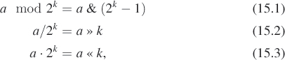
for fixed-point values. Here we use » as the operator to shift the bits of the left operand to the right by the value of the right operand, and & as the bitwise AND operator.
This is one reason that many graphics APIs historically required power-of-two image dimensions (another is MIP mapping). One can always express a number that is not a power of two as the sum of multiple powers of two. In fact, that’s what binary encoding does! For example, 640 = 512 + 128, so x + 640y = x + (y«9) + (y«7).
Implement forward and backward mappings from integer (x, y) pixel locations to 1D array indices i, for a typical HD resolution of 1920 × 1080, using only bitwise operations, addition, and subtraction.
Familiarity with the bit-manipulation methods for mapping between 1D and 2D arrays is important now so that you can understand other people’s code. It will also help you to appreciate how hardware-accelerated rendering might implement some low-level operations and why a rendering API might have certain constraints. However, this kind of micro-optimization will not substantially affect the performance of your renderer at this stage, so it is not yet worth including.
Our Image class stores physically meaningful values. The natural measurement of the light arriving along a ray is in terms of radiance, whose definition and precise units are described in Chapter 26. The image typically represents the light about to fall onto each pixel of a sensor or area of a piece of film. It doesn’t represent the sensor response process.
Displays and image files tend to work with arbitrarily scaled 8-bit display values that map nonlinearly to radiance. For example, if we set the display pixel value to 64, the display pixel does not emit twice the radiance that it does when we set the same pixel to 32. This means that we cannot display our image faithfully by simply rescaling radiance to display values. In fact, the relationship involves an exponent commonly called gamma, as described briefly below and at length in Section 28.12.
Assume some multiplicative factor d that rescales the radiance values in an image so that the largest value we wish to represent maps to 1.0 and the smallest maps to 0.0. This fills the role of the camera’s shutter and aperture. The user will select this value as part of the scene definition. Mapping it to a GUI slider is often a good idea.
Historically, most images stored 8-bit values whose meanings were illspecified. Today it is more common to specify what they mean. An image that actually stores radiance values is informally said to store linear radiance, indicating that the pixel value varies linearly with the radiance (see Chapter 17). Since the radiance range of a typical outdoor scene with shadows might span six orders of magnitude, the data would suffer from perceptible quantization artifacts were it reduced to eight bits per channel. However, human perception of brightness is roughly logarithmic. This means that distributing precision nonlinearly can reduce the perceptual error of a small bit-depth approximation. Gamma encoding is a common practice for distributing values according to a fractional power law, where 1/γ is the power. This encoding curve roughly matches the logarithmic response curve of the human visual system. Most computer displays accept input already gamma-encoded along the sRGB standard curve, which is about γ = 2.2. Many image file formats, such as PPM, also default to this gamma encoding. A routine that maps a radiance value to an 8-bit display value with a gamma value of 2.2 is:
1 int Image::PPMGammaEncode(float radiance, float d) const {
2 return int(pow(std::min(1.0f, std::max(0.0f, radiance * d)),
3 1.0f / 2.2f) * 255.0f);
4 }
Note that x1/2.2 ≈ ![]() . Because they are faster than arbitrary exponentiation on most hardware, square root and square are often employed in real-time rendering as efficient γ = 2.0 encoding and decoding methods.
. Because they are faster than arbitrary exponentiation on most hardware, square root and square are often employed in real-time rendering as efficient γ = 2.0 encoding and decoding methods.
The save routine is our bare-bones method for exporting data from the renderer for viewing. It saves the image in human-readable PPM format [P+ 10] and is implemented in Listing 15.6.
Listing 15.6: Saving an image to an ASCII RGB PPM file.
1 void Image::save(const std::string& filename, float d) const {
2 FILE* file = fopen(filename.c_str(), "wt");
3 fprintf(file, "P3 %d %d 255
", m_width, m_height);
4 for (int y = 0; y < m_height; ++y) {
5 fprintf(file, "
# y = %d
", y);
6 for (int x = 0; x < m_width; ++x) {
7 const Radiance3& c(get(x, y));
8 fprintf(file, "%d %d %d
",
9 PPMGammaEncode(c.r, d),
10 PPMGammaEncode(c.g, d),
11 PPMGammaEncode(c.b, d));
12 }
13 }
14 fclose(file);
15 }
This is a useful snippet of code beyond its immediate purpose of saving an image. The structure appears frequently in 2D graphics code. The outer loop iterates over rows. It contains any kind of per-row computation (in this case, printing the row number). The inner loop iterates over the columns of one row and performs the per-pixel operations. Note that if we wished to amortize the cost of computing y * m_width inside the get routine, we could compute that as a perrow operation and merely accumulate the 1-pixel offsets in the inner loop. We do not do so in this case because that would complicate the code without providing a measurable performance increase, since writing a formatted text file would remain slow compared to performing one multiplication per pixel.
The PPM format is slow for loading and saving, and consumes lots of space when storing images. For those reasons, it is rarely used outside academia. However, it is convenient for data interchange between programs. It is also convenient for debugging small images for three reasons. The first is that it is easy to read and write. The second is that many image programs and libraries support it, including Adobe Photoshop and xv. The third is that we can open it in a text editor to look directly at the (gamma-corrected) pixel values.
After writing the image-saving code, we displayed the simple pattern shown in Figure 15.2 as a debugging aid. If you implement your own image saving or display mechanism, consider doing something similar. The test pattern alternates dark blue pixels with ones that form a gradient. The reason for creating the single-pixel checkerboard pattern is to verify that the image was neither stretched nor cropped during display. If it was, then one or more thin horizontal or vertical lines would appear. (If you are looking at this image on an electronic display, you may see such patterns, indicating that your viewing software is indeed stretching it.) The motivation for the gradient is to determine whether gamma correction is being applied correctly. A linear radiance gradient should appear as a nonlinear brightness gradient, when displayed correctly. Specifically, it should primarily look like the brighter shades. The pattern on the left is shown without gamma correction. The gradient appears to have linear brightness, indicating that it is not displayed correctly. The pattern on the right is shown with gamma correction. The gradient correctly appears to be heavily shifted toward the brighter shaders.
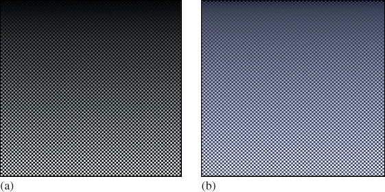
Figure 15.2: A pattern for testing the Image class. The pattern is a checkerboard of 1-pixel squares that alternate between 1/10 W/(m2 sr) in the blue channel and a vertical gradient from 0 to 10. (a) Viewed with deviceGamma = 1.0 and displayConstant = 1.0, which makes dim squares appear black and gives the appearance of a linear change in brightness. (b) Displayed more correctly with deviceGamma = 2.0, where the linear radiance gradient correctly appears as a nonlinear brightness ramp and the dim squares are correctly visible. (The conversion to a printed image or your online image viewer may further affect the image.)
Note that we made the darker squares blue, yet in the left pattern—without gamma correction—they appear black. That is because gamma correction helps make darker shades more visible, as in the right image. This hue shift is another argument for being careful to always implement gamma correction, beyond the tone shift. Of course, we don’t know the exact characteristics of the display (although one can typically determine its gamma exponent) or the exact viewing conditions of the room, so precise color correction and tone mapping is beyond our ability here. However, the simple act of applying gamma correction arguably captures some of the most important aspects of that process and is computationally inexpensive and robust.
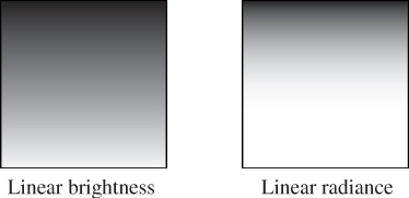
Two images are shown below. Both have been gamma-encoded with γ = 2.0 for printing and online display. The image on the left is a gradient that has been rendered to give the impression of linear brightness. It should appear as a linear color ramp. The image on the right was rendered with linear radiance (it is the checkerboard on the right of Figure 15.2 without the blue squares). It should appear as a nonlinear color ramp. The image was rendered at 200 × 200 pixels. What equation did we use to compute the value (in [0, 1]) of the pixel at (x, y) for the gradient image on the left?
15.3.3. Scene Representation
Listing 15.7 shows a Triangle class. It stores each triangle by explicitly storing each vertex. Each vertex has an associated normal that is used exclusively for shading; the normals do not describe the actual geometry. These are sometimes called shading normals. When the vertex normals are identical to the normal to the plane of the triangle, the triangle’s shading will appear consistent with its actual geometry. When the normals diverge from this, the shading will mimic that of a curved surface. Since the silhouette of the triangle will still be polygonal, this effect is most convincing in a scene containing many small triangles.
Listing 15.7: Interface for a Triangle class.
1 class Triangle {
2 private:
3 Point3 m_vertex[3];
4 Vector3 m_normal[3];
5 BSDF m_bsdf;
6
7 public:
8
9 const Point3& vertex(int i) const { return m_vertex[i]; }
10 const Vector3& normal(int i) const { return m_normal[i]; }
11 const BSDF& bsdf() const { return m_bsdf; }
12 ...
13 };
We also associate a BSDF class value with each triangle. This describes the material properties of the surface modeled by the triangle. It is described in Section 15.4.5. For now, think of this as the color of the triangle.
The representation of the triangle is concealed by making the member variables private. Although the implementation shown contains methods that simply return those member variables, you will later use this abstraction boundary to create a more efficient implementation of the triangle. For example, many triangles may share the same vertices and bidirectional scattering distribution functions (BSDFs), so this representation is not very space-efficient. There are also properties of the triangle, such as the edge lengths and geometric normal, that we will find ourselves frequently recomputing and could benefit from storing explicitly.
Compute the size in bytes of one Triangle. How big is a 1M triangle mesh? Is that reasonable? How does this compare with the size of a stored mesh file, say, in the binary 3DS format or the ASCII OBJ format? What are other advantages, beyond space reduction, of sharing vertices between triangles in a mesh?
Listing 15.8 shows our implementation of an omnidirectional point light source. We represent the power it emits at three wavelengths (or in three wavelength bands), and the center of the emitter. Note that emitters are infinitely small in our representation, so they are not themselves visible. If we wish to see the source appear in the final rendering we need to either add geometry around it or explicitly render additional information into the image. We will do neither explicitly in this chapter, although you may find that these are necessary when debugging your illumination code.
Listing 15.8: Interface for a uniform point luminaire—a light source.
1 class Light {
2 public:
3 Point3 position;
4
5 /** Over the entire sphere. */
6 Power3 power;
7 };
Listing 15.9 describes the scene as sets of triangles and lights. Our choice of arrays for the implementation of these sets imposes an ordering on the scene. This is convenient for ensuring a reproducible environment for debugging. However, for now we are going to create that ordering in an arbitrary way, and that choice may affect performance and even our image in some slight ways, such as resolving ties between which surface is closest at an intersection. More sophisticated scene data structures may include additional structure in the scene and impose a specific ordering.
Listing 15.9: Interface for a scene represented as an unstructured list of triangles and light sources.
1 class Scene {
2 public:
3 std::vector<Triangle> triangleArray;
4 std::vector<Light> lightArray;
5 };
Listing 15.10 represents our camera. The camera has a pinhole aperture, an instantaneous shutter, and artificial near and far planes of constant (negative) z values. We assume that the camera is located at the origin and facing along the –z-axis.
Listing 15.10: Interface for a pinhole camera at the origin.
1 class Camera {
2 public:
3 float zNear;
4 float zFar;
5 float fieldOfViewX;
6
7 Camera() : zNear(-0.1f), zFar(-100.0f), fieldOfViewX(PI / 2.0f) {}
8 };
We constrain the horizontal field of view of the camera to be fieldOfViewX. This is the measure of the angle from the center of the leftmost pixel to the center of the rightmost pixel along the horizon in the camera’s view in radians (it is shown later in Figure 15.3). During rendering, we will compute the aspect ratio of the target image and implicitly use that to determine the vertical field of view. We could alternatively specify the vertical field of view and compute the horizontal field of view from the aspect ratio.
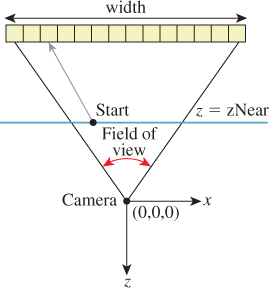
Figure 15.3: The ray through a pixel center in terms of the image resolution and the camera’s horizontal field of view.
15.3.4. A Test Scene
We’ll test our renderers on a scene that contains one triangle whose vertices are
Point3(0,1,-2), Point3(-1.9,-1,-2), and Point3(1.6,-0.5,-2),
and whose vertex normals are
Vector3( 0.0f, 0.6f, 1.0f).direction(),
Vector3(-0.4f,-0.4f, 1.0f).direction(), and
Vector3( 0.4f,-0.4f, 1.0f).direction().
We create one light source in the scene, located at Point3(1.0f,3.0f,1.0f) and emitting power Power3(10, 10, 10). The camera is at the origin and is facing along the –z-axis, with y increasing upward in screen space and x increasing to the right. The image has size 800 × 500 and is initialized to dark blue.
This choice of scene data was deliberate, because when debugging it is a good idea to choose configurations that use nonsquare aspect ratios, nonprimary colors, asymmetric objects, etc. to help find cases where you have accidentally swapped axes or color channels. Having distinct values for the properties of each vertex also makes it easier to track values through code. For example, on this triangle, you can determine which vertex you are examining merely by looking at its x-coordinate.
On the other hand, the camera is the standard one, which allows us to avoid transforming rays and geometry. That leads to some efficiency and simplicity in the implementation and helps with debugging because the input data maps exactly to the data rendered, and in practice, most rendering algorithms operate in the camera’s reference frame anyway.
Mandatory; do not continue until you have done this: Draw a schematic diagram of this scene from three viewpoints.
1. The orthographic view from infinity facing along the x-axis. Make z increase to the right and y increase upward. Show the camera and its field of view.
2. The orthographic view from infinity facing along the –y-axis. Make x increase to the right and z increase downward. Show the camera and its field of view. Draw the vertex normals.
3. The perspective view from the camera, facing along the –z-axis; the camera should not appear in this image.
15.4. A Ray-Casting Renderer
We begin the ray-casting renderer by expanding and implementing our initial pseudocode from Listing 15.2. It is repeated in Listing 15.11 with more detail.
Listing 15.11: Detailed pseudocode for a ray-casting renderer.
1 for each pixel row y:
2 for each pixel column x:
3 let R = ray through screen space position (x + 0.5, y + 0.5)
4 closest = ∞
5 for each triangle T:
6 d = intersect(T, R)
7 if (d < closest)
8 closest = d
9 sum = 0
10 let P be the intersection point
11 for each direction ωi:
12 sum += light scattered at P from ωi to ωo
13
14 image[x, y] = sum
The three loops iterate over every ray and triangle combination. The body of the for-each-triangle loop verifies that the new intersection is closer than previous observed ones, and then shades the intersection. We will abstract the operation of ray intersection and sampling into a helper function called sampleRayTriangle. Listing 15.12 gives the interface for this helper function.
Listing 15.12: Interface for a function that performs ray-triangle intersection and shading.
1 bool sampleRayTriangle(const Scene& scene, int x, int y,
2 const Ray& R, const Triangle& T,
3 Radiance3& radiance, float& distance);
The specification for sampleRayTriangle is as follows. It tests a particular ray against a triangle. If the intersection exists and is closer than all previously observed intersections for this ray, it computes the radiance scattered toward the viewer and returns true. The innermost loop therefore sets the value of pixel (x, y) to the radiance L_o passing through its center from the closest triangle. Radiance from farther triangles is not interesting because it will (conceptually) be blocked by the back of the closest triangle and never reach the image. The implementation of sampleRayTriangle appears in Listing 15.15.
To render the entire image, we must invoke sampleRayTriangle once for each pixel center and for each triangle. Listing 15.13 defines rayTrace, which performs this iteration. It takes as arguments a box within which to cast rays (see Section 15.4.4). We use L_o to denote the radiance from the triangle; the subscript “o” is for “outgoing”.
Listing 15.13: Code to trace one ray for every pixel between (x0, y0) and (x1-1, y1-1), inclusive.
1 /** Trace eye rays with origins in the box from [x0, y0] to (x1, y1).*/
2 void rayTrace(Image& image, const Scene& scene,
3 const Camera& camera, int x0, int x1, int y0, int y1) {
4
5 // For each pixel
6 for (int y = y0; y < y1; ++y) {
7 for (int x = y0; x < x1; ++x) {
8
9 // Ray through the pixel
10 const Ray& R = computeEyeRay(x + 0.5f, y + 0.5f, image.width(),
11 image.height(), camera);
12
13 // Distance to closest known intersection
14 float distance = INFINITY;
15 Radiance3 L_o;
16
17 // For each triangle
18 for (unsigned int t = 0; t < scene.triangleArray.size(); ++t){
19 const Triangle& T = scene.triangleArray[t];
20
21 if (sampleRayTriangle(scene, x, y, R, T, L_o, distance)) {
22 image.set(x, y, L_o);
23 }
24 }
25 }
26 }
27 }
To invoke rayTrace on the entire image, we will use the call:
rayTrace(image, scene, camera, 0, image.width(), 0, image.height());
15.4.1. Generating an Eye Ray
Assume the camera’s center of projection is at the origin, (0, 0, 0), and that, in the camera’s frame of reference, the y-axis points upward, the x-axis points to the right, and the z-axis points out of the screen. Thus, the camera is facing along its own –z-axis, in a right-handed coordinate system. We can transform any scene to this coordinate system using the transformations from Chapter 11.
We require a utility function, computeEyeRay, to find the ray through the center of a pixel, which in screen space is given by (x + 0.5, y + 0.5) for integers x and y. Listing 15.14 gives an implementation. The key geometry is depicted in Figure 15.3. The figure is a top view of the scene in which x increases to the right and z increases downward. The near plane appears as a horizontal line, and the start point is on that plane, along the line from the camera at the origin to the center of a specific pixel.
To implement this function we needed to parameterize the camera by either the image plane depth or the desired field of view. Field of view is a more intuitive way to specify a camera, so we previously chose that parameterization when building the scene representation.
Listing 15.14: Computing the ray through the center of pixel (x, y) on a width × height image.
1 Ray computeEyeRay(float x, float y, int width, int height, const Camera& camera) {
2 const float aspect = float(height) / width;
3
4 // Compute the side of a square at z = -1 based on our
5 // horizontal left-edge-to-right-edge field of view
6 const float s = -2.0f * tan(camera.fieldOfViewX * 0.5f);
7
8 const Vector3& start =
9 Vector3( (x / width - 0.5f) * s,
10 -(y / height - 0.5f) * s * aspect, 1.0f) * camera.zNear;
11
12 return Ray(start, start.direction());
13 }
We choose to place the ray origin on the near (sometimes called hither) clipping plane, at z = camera.zNear. We could start rays at the origin instead of the near plane, but starting at the near plane will make it easier for results to line up precisely with our rasterizer later.
The ray direction is the direction from the center of projection (which is at the origin, (0, 0, 0)) to the ray start point, so we simply normalize start point.
By the rules of Chapter 7, we should compute the ray direction as (start - Vector3(0,0,0)).direction(). That makes the camera position explicit, so we are less likely to introduce a bug if we later change the camera. This arises simply from strongly typing the code to match the underlying mathematical types. On the other hand, our code is going to be full of lines like this, and consistently applying correct typing might lead to more harm from obscuring the algorithm than benefit from occasionally finding an error. It is a matter of personal taste and experience (we can somewhat reconcile our typing with the math by claiming that P.direction() on a point P returns the direction to the point, rather than “normalizing” the point).
Rewrite computeEyeRay using the distinct Point and Vector abstractions from Chapter 7 to get a feel for how this affects the presentation and correctness. If this inspires you, it’s quite reasonable to restructure all the code in this chapter that way, and doing so is a valuable exercise.
Note that the y-coordinate of the start is negated. This is because y is in 2D screen space, with a “y = down” convention, and the ray is in a 3D coordinate system with a “y = up” convention.
To specify the vertical field of view instead of the horizontal one, replace fieldOfViewX with fieldOfViewY and insert the line s /= aspect.
15.4.1.1. Camera Design Notes
The C++ language offers both functions and methods as procedural abstractions. We have presented computeEyeRay as a function that takes a Camera parameter to distinguish the “support code” Camera class from the ray-tracer-specific code that you are adding. As you move forward through the book, consider refactoring the support code to integrate auxiliary functions like this directly into the appropriate classes. (If you are using an existing 3D library as support code, it is likely that the provided camera class already contains such a method. In that case, it is worth implementing the method once as a function here so that you have the experience of walking through and debugging the routine. You can later discard your version in favor of a canonical one once you’ve reaped the educational value.)
A software engineering tip: Although we have chosen to forgo small optimizations, it is still important to be careful to use references (e.g., Image&) to avoid excess copying of arguments and intermediate results. There are two related reasons for this, and neither is about the performance of this program.
The first reason is that we want to be in the habit of avoiding excessive copying. A Vector3 occupies 12 bytes of memory, but a full-screen Image is a few megabytes. If we’re conscientious about never copying data unless we want copy semantics, then we won’t later accidentally copy an Image or other large structure. Memory allocation and copy operations can be surprisingly slow and will bloat the memory footprint of our program. The time cost of copying data isn’t just a constant overhead factor on performance. Copying the image once per pixel, in the inner loop, would change the ray caster’s asymptotic run time from Ο(n) in the number of pixels to Ο(n2).
The second reason is that experienced programmers rely on a set of idioms that are chosen to avoid bugs. Any deviation from those attracts attention, because it is a potential bug. One such convention in C++ is to pass each value as a const reference unless otherwise required, for the long-term performance reasons just described. So code that doesn’t do so takes longer for an experienced programmer to review because of the need to check that there isn’t an error or performance implication whenever an idiom is not followed. If you are an experienced C++ programmer, then such idioms help you to read the code. If you are not, then either ignore all the ampersands and treat this as pseudocode, or use it as an opportunity to become a better C++ programmer.
15.4.1.2. Testing the Eye-Ray Computation
We need to test computeEyeRay before continuing. One way to do this is to write a unit test that computes the eye rays for specific pixels and then compares them to manually computed results. That is always a good testing strategy. In addition to that, we can visualize the eye rays. Visualization is a good way to quickly see the result of many computations. It allows us to more intuitively check results, and to identify patterns of errors if they do not match what we expected.
In this section, we’ll visualize the directions of the rays. The same process can be applied to the origins. The directions are the more common location for an error and conveniently have a bounded range, which make them both more important and easier to visualize.
A natural scheme for visualizing a direction is to interpret the (x, y, z) fields as (r, g, b) color triplets. The conversion of ray direction to pixel color is of course a gross violation of units, but it is a really useful debugging technique and we aren’t expecting anything principled here anyway.
Because each ordinate is on the interval [–1, 1], we rescale them to the range [0, 1] by r = (x + 1)/2. Our image display routines also apply an exposure function, so we need to scale the resultant intensity down by a constant on the order of the inverse of the exposure value. Temporarily inserting the following line:
image.set(x, y, Color3(R.direction() + Vector3(1, 1, 1)) / 5);
into rayTrace in place of the sampleRayTriangle call should yield an image like that shown in Figure 15.4. (The factor of 1/5 scales the debugging values to a reasonable range for our output, which was originally calibrated for radiance; we found a usable constant for this particular example by trial and error.) We expect the x-coordinate of the ray, which here is visualized as the color red, to increase from a minimum on the left to a maximum on the right. Likewise, the (3D) y-coordinate, which is visualized as green, should increase from a minimum at the bottom of the image to a maximum at the top. If your result varies from this, examine the pattern you observe and consider what kind of error could produce it. We will revisit visualization as a debugging technique later in this chapter, when testing the more complex intersection routine.

15.4.2. Sampling Framework: Intersect and Shade
Listing 15.15 shows the code for sampling a triangle with a ray. This code doesn’t perform any of the heavy lifting itself. It just computes the values needed for intersect and shade.
Listing 15.15: Sampling the intersection and shading of one triangle with one ray.
1 bool sampleRayTriangle(const Scene& scene, int x, int y, const Ray& R,
const Triangle& T, Radiance3& radiance, float& distance) {
2
3 float weight[3];
4 const float d = intersect(R, T, weight);
5
6 if (d >= distance) {
7 return false;
8 }
9
10 // This intersection is closer than the previous one
11 distance = d;
12
13 // Intersection point
14 const Point3& P = R.origin() + R.direction() * d;
15
16 // Find the interpolated vertex normal at the intersection
17 const Vector3& n = (T.normal(0) * weight[0] +
18 T.normal(1) * weight[1] +
19 T.normal(2) * weight[2]).direction();
20
21 const Vector3& w_o = -R.direction();
22
23 shade(scene, T, P, n, w_o, radiance);
24
25 // Debugging intersect: set to white on any intersection
26 //radiance = Radiance3(1, 1, 1);
27
28 // Debugging barycentric
29 //radiance = Radiance3(weight[0], weight[1], weight[2]) / 15;
30
31 return true;
32 }
The sampleRayTriangle routine returns false if there was no intersection closer than distance; otherwise, it updates distance and radiance and returns true.
When invoking this routine, the caller passes the distance to the closest currently known intersection, which is initially INFINITY (let INFINITY = std::numeric_limits<T>::infinity() in C++, or simply 1.0/0.0). We will design the intersect routine to return INFINITY when no intersection exists between R and T so that a missed intersection will never cause sampleRayTriangle to return true.
Placing the (d >= distance) test before the shading code is an optimization. We would still obtain correct results if we always computed the shading before testing whether the new intersection is in fact the closest. This is an important optimization because the shade routine may be arbitrarily expensive. In fact, in a full-featured ray tracer, almost all computation time is spent inside shade, which recursively samples additional rays. We won’t discuss further shading optimizations in this chapter, but you should be aware of the importance of an early termination when another surface is known to be closer.
Note that the order of the triangles in the calling routine (rayTrace) affects the performance of the routine. If the triangles are in back-to-front order, then we will shade each one, only to reject all but the closest. This is the worst case. If the triangles are in front-to-back order, then we will shade the first and reject the rest without further shading effort. We could ensure the best performance always by separating sampleRayTriangle into two auxiliary routines: one to find the closest intersection and one to shade that intersection. This is a common practice in ray tracers. Keep this in mind, but do not make the change yet. Once we have written the rasterizer renderer, we will consider the space and time implications of such optimizations under both ray casting and rasterization, which gives insights into many variations on each algorithm.
We’ll implement and test intersect first. To do so, comment out the call to shade on line 23 and uncomment either of the debugging lines below it.
15.4.3. Ray-Triangle Intersection
We’ll find the intersection of the eye ray and a triangle in two steps, following the method described in Section 7.9 and implemented in Listing 15.16. This method first intersects the line containing the ray with the plane containing the triangle. It then solves for the barycentric weights to determine if the intersection is within the triangle. We need to ignore intersections with the back of the single-sided triangle and intersections that occur along the part of the line that is not on the ray.
The same weights that we use to determine if the intersection is within the triangle are later useful for interpolating per-vertex properties, such as shading normals. We structure our implementation to return the weights to the caller. The caller could use either those or the distance traveled along the ray to find the intersection point. We return the distance traveled because we know that we will later need that anyway to identify the closest intersection to the viewer in a scene with many triangles. We return the barycentric weights for use in interpolation.
Figure 15.5 shows the geometry of the situation. Let R be the ray and T be the triangle. Let ![]() be the edge vector from V0 to V1 and
be the edge vector from V0 to V1 and ![]() be the edge vector from V0 to V2. Vector
be the edge vector from V0 to V2. Vector ![]() is orthogonal to both the ray and
is orthogonal to both the ray and ![]() . Note that if
. Note that if ![]() is also orthogonal to
is also orthogonal to ![]() , then the ray is parallel to the triangle and there is no intersection. If
, then the ray is parallel to the triangle and there is no intersection. If ![]() is in the negative hemisphere of
is in the negative hemisphere of ![]() (i.e., “points away”), then the ray travels away from the triangle.
(i.e., “points away”), then the ray travels away from the triangle.
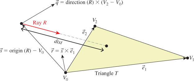
Vector ![]() is the displacement of the ray origin from V0, and vector
is the displacement of the ray origin from V0, and vector ![]() is the cross product of
is the cross product of ![]() and
and ![]() . These vectors are used to construct the barycentric weights, as shown in Listing 15.16.
. These vectors are used to construct the barycentric weights, as shown in Listing 15.16.
Variable a is the rate at which the ray is approaching the triangle, multiplied by twice the area of the triangle. This is not obvious from the way it is computed here, but it can be seen by applying a triple-product identity relation:
since the direction of ![]() 2 ×
2 × ![]() 1 is opposite the triangle’s geometric normal n. The particular form of this expression chosen in the implementation is convenient because the
1 is opposite the triangle’s geometric normal n. The particular form of this expression chosen in the implementation is convenient because the q vector is needed again later in the code for computing the barycentric weights.
There are several cases where we need to compare a value against zero. The two epsilon constants guard these comparisons against errors arising from limited numerical precision.
The comparison a <= epsilon detects two cases. If a is zero, then the ray is parallel to the triangle and never intersects it. In this case, the code divided by zero many times, so other variables may be infinity or not-a-number. That’s irrelevant, since the first test expression will still make the entire test expression true. If a is negative, then the ray is traveling away from the triangle and will never intersect it. Recall that a is the rate at which the ray approaches the triangle, multiplied by the area of the triangle. If epsilon is too large, then intersections with triangles will be missed at glancing angles, and this missed intersection behavior will be more likely to occur at triangles with large areas than at those with small areas. Note that if we changed the test to fabs(a)<= epsilon, then triangles would have two sides. This is not necessary for correct models of real, opaque objects; however, for rendering mathematical models or models with errors in them it can be convenient. Later we will depend on optimizations that allow us to quickly cull the (approximately half) of the scene representing back faces, so we choose to render single-sided triangles here for consistency.
Listing 15.16: Ray-triangle intersection (derived from [MT97])
1 float intersect(const Ray& R, const Triangle& T, float weight[3]) {
2 const Vector3& e1 = T.vertex(1) - T.vertex(0);
3 const Vector3& e2 = T.vertex(2) - T.vertex(0);
4 const Vector3& q = R.direction().cross(e2);
5
6 const float a = e1.dot(q);
7
8 const Vector3& s = R.origin() - T.vertex(0);
9 const Vector3& r = s.cross(e1);
10
11 // Barycentric vertex weights
12 weight[1] = s.dot(q) / a;
13 weight[2] = R.direction().dot(r) / a;
14 weight[0] = 1.0f - (weight[1] + weight[2]);
15
16 const float dist = e2.dot(r) / a;
17
18 static const float epsilon = 1e-7f;
19 static const float epsilon2 = 1e-10;
20
21 if ((a <= epsilon) || (weight[0] < -epsilon2) ||
22 (weight[1] < -epsilon2) || (weight[2] < -epsilon2) ||
23 (dist <= 0.0f)) {
24 // The ray is nearly parallel to the triangle, or the
25 // intersection lies outside the triangle or behind
26 // the ray origin: "infinite" distance until intersection.
27 return INFINITY;
28 } else {
29 return dist;
30 }
31 }
The epsilon2 constant allows a ray to intersect a triangle slightly outside the bounds of the triangle. This ensures that triangles that share an edge completely cover pixels along that edge despite numerical precision limits. If epsilon2 is too small, then single-pixel holes will very occasionally appear on that edge. If it is too large, then all triangles will visibly appear to be too large.
Depending on your processor architecture, it may be faster to perform an early test and potential return rather than allowing not-a-number and infinity propagation in the ill-conditioned case where a ≈ 0. Many values can also be precomputed, for example, the edge lengths of the triangle, or at least be reused within a single intersection, for example, 1.0f / a. There’s a cottage industry of optimizing this intersection code for various architectures, compilers, and scene types (e.g., [MT97] for scalar processors versus [WBB08] for vector processors). Let’s forgo those low-level optimizations and stick to high-level algorithmic decisions. In practice, most ray casters spend very little time in the ray intersection code anyway. The fastest way to determine if a ray intersects a triangle is to never ask that question in the first place. That is, in Chapter 37, we will introduce data structures that quickly and conservatively eliminate whole sets of triangles that the ray could not possibly intersect, without ever performing the ray-triangle intersection. So optimizing this routine now would only complicate it without affecting our long-term performance profile.
Our renderer only processes triangles. We could easily extend it to render scenes containing any kind of primitive for which we can provide a ray intersection solution. Surfaces defined by low-order equations, like the plane, rectangle, sphere, and cylinder, have explicit solutions. For others, such as bicubic patches, we can use root-finding methods.
15.4.4. Debugging
We now verify that the intersection code code is correct. (The code we’ve given you is correct, but if you invoked it with the wrong parameters, or introduced an error when porting to a different language or support code base, then you need to learn how to find that error.) This is a good opportunity for learning some additional graphics debugging tricks, all of which demonstrate the Visual Debugging principle.
It would be impractical to manually examine every intersection result in a debugger or printout. That is because the rayTrace function invokes intersect thousands of times. So instead of examining individual results, we visualize the barycentric coordinates by setting the radiance at a pixel to be proportional to the barycentric coordinates following the Visual Debugging principle. Figure 15.6 shows the correct resultant image. If your program produces a comparable result, then your program is probably nearly correct.
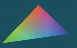
Figure 15.6: The single triangle scene visualized with color equal to barycentric weight for debugging the intersection code.
What should you do if your result looks different? You can’t examine every result, and if you place a breakpoint in intersect, then you will have to step through hundreds of ray casts that miss the triangle before coming to the interesting intersection tests.
This is why we structured rayTrace to trace within a caller-specified rectangle, rather than the whole image. We can invoke the ray tracer on a single pixel from main(), or better yet, create a debugging interface where clicking on a pixel with the mouse invokes the single-pixel trace on the selected pixel. By setting breakpoints or printing intermediate results under this setup, we can investigate why an artifact appears at a specific pixel. For one pixel, the math is simple enough that we can also compute the desired results by hand and compare them to those produced by the program.
In general, even simple graphics programs tend to have large amounts of data. This may be many triangles, many pixels, or many frames of animation. The processing for these may also be running on many threads, or on a GPU. Traditional debugging methods can be hard to apply in the face of such numerous data and massive parallelism. Furthermore, the graphics development environment may preclude traditional techniques such as printing output or setting breakpoints. For example, under a hardware rendering API, your program is executing on an embedded processor that frequently has no access to the console and is inaccessible to your debugger.
Fortunately, three strategies tend to work well for graphics debugging.
1. Use assertions liberally. These cost you nothing in the optimized version of the program, pass silently in the debug version when the program operates correctly, and break the program at the test location when an assertion is violated. Thus, they help to identify failure cases without requiring that you manually step through the correct cases.
2. Immediately reduce to the minimal test case. This is often a single-triangle scene with a single light and a single pixel. The trick here is to find the combination of light, triangle, and pixel that produces incorrect results. Assertions and the GUI click-to-debug scheme work well for that.
3. Visualize intermediate results. We have just rendered an image of the barycentric coordinates of eye-ray intersections with a triangle for a 400,000-pixel image. Were we to print out these values or step through them in the debugger, we would have little chance of recognizing an incorrect value in that mass of data. If we see, for example, a black pixel, or a white pixel, or notice that the red and green channels are swapped, then we may be able to deduce the nature of the error that caused this, or at least know which inputs cause the routine to fail.
15.4.5. Shading
We are now ready to implement shade. This routine computes the incident radiance at the intersection point P and how much radiance scatters back along the eye ray to the viewer.
Let’s consider only light transport paths directly from the source to the surface to the camera. Under this restriction, there is no light arriving at the surface from any directions except those to the lights. So we only need to consider a finite number of ωi values. Let’s also assume for the moment that there is always a line of sight to the light. This means that there will (perhaps incorrectly) be no shadows in the rendered image.
Listing 15.17 iterates over the light sources in the scene (note that we have only one in our test scene). For each light, the loop body computes the distance and direction to that light from the point being shaded. Assume that lights emit uniformly in all directions and are at finite locations in the scene. Under these assumptions, the incident radiance L_i at point P is proportional to the total power of the source divided by the square of the distance between the source and P. This is because at a given distance, the light’s power is distributed equally over a sphere of that radius. Because we are ignoring shadowing, let the visible function always return true for now. In the future it will return false if there is no line of sight from the source to P, in which case the light should contribute no incident radiance.
The outgoing radiance to the camera, L_o, is the sum of the fraction of incident radiance that scatters in that direction. We abstract the scattering function into a BSDF. We implement this function as a class so that it can maintain state across multiple invocations and support an inheritance hierarchy. Later in this book, we will also find that it is desirable to perform other operations beyond invoking this function; for example, we might want to sample with respect to the probability distribution it defines. Using a class representation will allow us to later introduce additional methods for these operations.
The evaluateFiniteScatteringDensity method of that class evaluates the scattering function for the given incoming and outgoing angles. We always then take the product of this and the incoming radiance, modulated by the cosine of the angle between w_i and n to account for the projected area over which incident radiance is distributed (by the Tilting principle).
Listing 15.17: The single-bounce shading code.
1 void shade(const Scene& scene, const Triangle& T, const Point3& P,
const Vector3& n, const Vector3& w_o, Radiance3& L_o) {
2
3 L_o = Color3(0.0f, 0.0f, 0.0f);
4
5 // For each direction (to a light source)
6 for (unsigned int i = 0; i < scene.lightArray.size(); ++i) {
7 const Light& light = scene.lightArray[i];
8
9 const Vector3& offset = light.position - P;
10 const float distanceToLight = offset.length();
11 const Vector3& w_i = offset / distanceToLight;
12
13 if (visible(P, w_i, distanceToLight, scene)) {
14 const Radiance3& L_i = light.power / (4 * PI * square(distanceToLight));
15
16 // Scatter the light
17 L_o +=
18 L_i *
19 T.bsdf().evaluateFiniteScatteringDensity(w_i, w_o) *
20 max(0.0, dot(w_i, n));
21 }
22 }
23 }
15.4.6. Lambertian Scattering
The simplest implementation of the BSDF assumes a surface appears to be the same brightness independent of the viewer’s orientation. That is, evaluateFiniteScatteringDensity returns a constant. This is called Lambertian reflectance, and it is a good model for matte surfaces such as paper and flat wall paint. It is also trivial to implement. Listing 15.18 gives the implementation (see Section 14.9.1 for a little more detail and Chapter 29 for a lot more). It has a single member, lambertian, that is the “color” of the surface. For energy conservation, this value should have all fields on the range [0, 1].
Listing 15.18: Lambertian BSDF implementation, following Listing 14.6.
1 class BSDF {
2 public:
3 Color3 k_L;
4
5 /** Returns f = L_o / (L_i * w_i.dot(n)) assuming
6 incident and outgoing directions are both in the
7 positive hemisphere above the normal */
8 Color3 evaluateFiniteScatteringDensity
9 (const Vector3& w_i, const Vector3& w_o) const {
10 return k_L / PI;
11 }
12 };
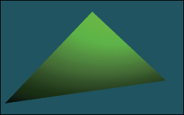
Figure 15.7 shows our triangle scene rendered with the Lambertian BSDF using k_L=Color3(0.0f, 0.0f, 0.8f). Because our triangle’s vertex normals are deflected away from the plane defined by the vertices, the triangle appears curved. Specifically, the bottom of the triangle is darker because the w_i.dot(n) term in line 20 of Listing 15.17 falls off toward the bottom of the triangle.
15.4.7. Glossy Scattering
The Lambertian surface appears dull because it has no highlight. A common approach for producing a more interesting shiny surface is to model it with something like the Blinn-Phong scattering function. An implementation of this function with the energy conservation factor from Sloan and Hoffmann [AMHH08, 257] is given in Listing 15.19. See Chapter 27 for a discussion of the origin of this function and alternatives to it. This is a variation on the shading function that we saw back in Chapter 6 in WPF, only now we are implementing it instead of just adjusting the parameters on a black box. The basic idea is simple: Extend the Lambertian BSDF with a large radial peak when the normal lies close to halfway between the incoming and outgoing directions. This peak is modeled by a cosine raised to a power since that is easy to compute with dot products. It is scaled so that the outgoing radiance never exceeds the incoming radiance and so that the sharpness and total intensity of the peak are largely independent parameters.
Listing 15.19: Blinn-Phong BSDF scattering density.
1 class BSDF {
2 public:
3 Color3 k_L;
4 Color3 k_G;
5 float s;
6 Vector3 n;
7 . . .
8
9 Color3 evaluateFiniteScatteringDensity(const Vector3& w_i,
10 const Vector3& w_o) const {
11 const Vector3& w_h = (w_i + w_o).direction();
12 return
13 (k_L + k_G * ((s + 8.0f) *
14 powf(std::max(0.0f, w_h.dot(n)), s) / 8.0f)) /
15 PI;
16
17 }
18 };
For this BSDF, choose lambertian + glossy < 1 at each color channel to ensure energy conservation, and glossySharpness typically in the range [0, 2000]. The glossySharpness is on a logarithmic scale, so it must be moved in larger increments as it becomes larger to have the same perceptual impact.
Figure 15.8 shows the green triangle rendered with the normalized Blinn-Phong BSDF. Here, k_L=Color3(0.0f, 0.0f, 0.8f), k_G=Color3(0.2f, 0.2f, 0.2f), and s=100.0f.
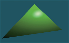
15.4.8. Shadows
The shade function in Listing 15.17 only adds the illumination contribution from a light source if there is an unoccluded line of sight between that source and the point P being shaded. Areas that are occluded are therefore darker. This absence of light is the phenomenon that we recognize as a shadow.
In our implementation, the line-of-sight visibility test is performed by the visible function, which is supposed to return true if and only if there is an unoccluded line of sight. While working on the shading routine we temporarily implemented visible to always return true, which means that our images contain no shadows. We now revisit the visible function in order to implement shadows.
We already have a powerful tool for evaluating line of sight: the intersect function. The light source is not visible from P if there is some intersection with another triangle. So we can test visibility simply by iterating over the scene again, this time using the shadow ray from P to the light instead of from the camera to P. Of course, we could also test rays from the light to P.
Listing 15.20 shows the implementation of visible. The structure is very similar to that of sampleRayTriangle. It has three major differences in the details. First, instead of shading the intersection, if we find any intersection we immediately return false for the visibility test. Second, instead of casting rays an infinite distance, we terminate when they have passed the light source. That is because we don’t care about triangles past the light—they could not possibly cast shadows on P. Third and finally, we don’t really start our shadow ray cast at P. Instead, we offset it slightly along the ray direction. This prevents the ray from reintersecting the surface containing P as soon as it is cast.
Listing 15.20: Line-of-sight visibility test, to be applied to shadow determination.
1 bool visible(const Vector3& P, const Vector3& direction, float
distance, const Scene& scene){
2 static const float rayBumpEpsilon = 1e-4;
3 const Ray shadowRay(P + direction * rayBumpEpsilon, direction);
4
5 distance -= rayBumpEpsilon;
6
7 // Test each potential shadow caster to see if it lies between P and the light
8 float ignore[3];
9 for (unsigned int s = 0; s < scene.triangleArray.size(); ++s) {
10 if (intersect(shadowRay, scene.triangleArray[s], ignore) < distance) {
11 // This triangle is closer than the light
12 return false;
13 }
14 }
15
16 return true;
17 }
Our single-triangle scene is insufficient for testing shadows. We require one object to cast shadows and another to receive them. A simple extension is to add a quadrilateral “ground plane” onto which the green triangle will cast its shadow. Listing 15.21 gives code to create this scene. Note that this code also adds another triangle with the same vertices as the green one but the opposite winding order. Because our triangles are single-sided, the green triangle would not cast a shadow. We need to add the back of that surface, which will occlude the rays cast upward toward the light from the ground.
Walk through the intersection code to verify the claim that without the second “side,” the green triangle would cast no shadow.
Figure 15.9 shows how the new scene should render before you implement shadows. If you do not see the ground plane under your own implementation, the most likely error is that you failed to loop over all triangles in one of the ray-casting routines.
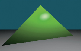
Figure 15.9: The green triangle scene extended with a two-triangle gray ground “plane.” A back surface has also been added to the green triangle.
Listing 15.21: Scene-creation code for a two-sided triangle and a ground plane.
1 void makeOneTriangleScene(Scene& s) { s.triangleArray.resize(1);
2
3 s.triangleArray[0] =
4 Triangle(Vector3(0,1,-2), Vector3(-1.9,-1,-2), Vector3(1.6,-0.5,-2),
5 Vector3(0,0.6f,1).direction(),
6 Vector3(-0.4f,-0.4f, 1.0f).direction(),
7 Vector3(0.4f,-0.4f, 1.0f).direction(),
8 BSDF(Color3::green() * 0.8f,Color3::white() * 0.2f, 100));
9
10 s.lightArray.resize(1);
11 s.lightArray[0].position = Point3(1, 3, 1);
12 s.lightArray[0].power = Color3::white() * 10.0f;
13 }
14
15 void makeTrianglePlusGroundScene(Scene& s) {
16 makeOneTriangleScene(s);
17
18 // Invert the winding of the triangle
19 s.triangleArray.push_back
20 (Triangle(Vector3(-1.9,-1,-2), Vector3(0,1,-2),
21 Vector3(1.6,-0.5,-2), Vector3(-0.4f,-0.4f, 1.0f).direction(),
22 Vector3(0,0.6f,1).direction(), Vector3(0.4f,-0.4f, 1.0f).direction(),
23 BSDF(Color3::green() * 0.8f,Color3::white() * 0.2f, 100)));
24
25 // Ground plane
26 const float groundY = -1.0f;
27 const Color3 groundColor = Color3::white() * 0.8f;
28 s.triangleArray.push_back
29 (Triangle(Vector3(-10, groundY, -10), Vector3(-10, groundY, -0.01f),
30 Vector3(10, groundY, -0.01f),
31 Vector3::unitY(), Vector3::unitY(), Vector3::unitY(), groundColor));
32
33 s.triangleArray.push_back
34 (Triangle(Vector3(-10, groundY, -10), Vector3(10, groundY, -0.01f),
35 Vector3(10, groundY, -10),
36 Vector3::unitY(), Vector3::unitY(), Vector3::unitY(), groundColor));
37 }
Figure 15.10 shows the scene rendered with visible implemented correctly. If the rayBumpEpsilon is too small, then shadow acne will appear on the green triangle. This artifact is shown in Figure 15.11. An alternative to starting the ray artificially far from P is to explicitly exclude the previous triangle from the shadow ray intersection computation. We chose not to do that because, while appropriate for unstructured triangles, it would be limiting to maintain that custom ray intersection code as our scene became more complicated. For example, we would like to later abstract the scene data structure from a simple array of triangles. The abstract data structure might internally employ a hash table or tree and have complex methods. Pushing the notion of excluding a surface into such a data structure could complicate that data structure and compromise its general-purpose use. Furthermore, although we are rendering only triangles now, we might wish to render other primitives in the future, such as spheres or implicit surfaces. Such primitives can intersect a ray multiple times. If we assume that the shadow ray never intersects the current surface, those objects would never self-shadow.

Figure 15.10: A four-triangle scene, with ray-cast shadows implemented via the visible function. The green triangle is two-sided.
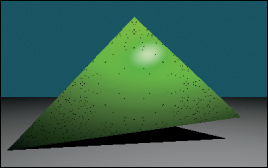
Figure 15.11: The dark dots on the green triangle are shadow acne caused by self-shadowing. This artifact occurs when the shadow ray immediately intersects the triangle that was being shaded.
15.4.9. A More Complex Scene
Now that we’ve built a renderer for one or two triangles, it is no more difficult to render scenes containing many triangles. Figure 15.12 shows a shiny, gold-colored teapot on a white ground plane. We parsed a file containing the vertices of the corresponding triangle mesh, appended those triangles to the Scene’s triangle array, and then ran the existing renderer on it. This scene contains about 100 triangles, so it renders about 100 times slower than the single-triangle scene. We can make arbitrarily more complex geometry and shading functions for the renderer. We are only limited by the quality of our models and our rendering performance, both of which will be improved in subsequent chapters.
This scene looks impressive (at least, relative to the single triangle) for two reasons. First, we see some real-world phenomena, such as shiny highlights, shadows, and nice gradients as light falls off. These occurred naturally from following the geometric relationships between light and surfaces in our implementation.
Second, the image resembles a recognizable object, specifically, a teapot. Unlike the illumination phenomena, nothing in our code made this look like a teapot. We simply loaded a triangle list from a data file that someone (originally, Jim Blinn) happened to have manually constructed. This teapot triangle list is a classic model in graphics. You can download the triangle mesh version used here from http://graphics.cs.williams.edu/data among other sources. Creating models like this is a separate problem from rendering, discussed in Chapter 22 and many others. Fortunately, there are many such models available, so we can defer the modeling problem while we discuss rendering.
We can learn a lesson from this. A strength and weakness of computer graphics as a technical field is that often the data contributes more to the quality of the final image than the algorithm. The same algorithm rendered the teapot and the green triangle, but the teapot looks more impressive because the data is better. Often a truly poor approximation algorithm will produce stunning results when a master artist creates the input—the commercial success of the film and game industries has largely depended on this fact. Be aware of this when judging algorithms based on rendered results, and take advantage of it by importing good artwork to demonstrate your own algorithms.
15.5. Intermezzo
To render a scene, we needed to iterate over both triangles and pixels. In the previous section, we arbitrarily chose to arrange the pixel loop on the outside and the triangle loop on the inside. That yielded the ray-casting algorithm. The ray-casting algorithm has three nice properties: It somewhat mimics the underlying physics, it separates the visibility routine from the shading routine, and it leverages the same ray-triangle intersection routine for both eye rays and shadow rays.
Admittedly, the relationship between ray casting and physics at the level demonstrated here is somewhat tenuous. Real photons propagate along rays from the light source to a surface to an eye, and we traced that path backward. Real photons don’t all scatter into the camera. Most photons from the light source scatter away from the camera, and much of the light that is scattered toward the camera from a surface didn’t arrive at that surface directly from the light. Nonetheless, an algorithm for sampling light along rays is a very good starting point for sampling photons, and it matches our intuition about how light should propagate. You can probably imagine improvements that would better model the true scattering behavior of light. Much of the rest of this book is devoted to such models.
In the next section, we invert the nesting order of the loops to yield a rasterizer algorithm. We then explore the implications of that change. We already have a working ray tracer to compare against. Thus, we can easily test the correctness of our changes by comparing against the ray-traced image and intermediate results. We also have a standard against which to measure the properties of the new algorithm. As you read the following section and implement the program that it describes, consider how the changes you are making affect code clarity, modularity, and efficiency. Particularly consider efficiency in both a wall-clock time and an asymptotic run time sense. Think about applications for which one of rasterization and ray casting is a better fit than the other.
These issues are not restricted to our choice of the outer loop. All high-performance renderers subdivide the scene and the image in sophisticated ways. The implementer must choose how to make these subdivisions and for each must again revisit whether to iterate first over pixels (i.e., ray directions) or triangles. The same considerations arise at every level, but they are evaluated differently based on the expected data sizes at that level and the machine architecture.
15.6. Rasterization
We now move on to implement the rasterizing renderer, and compare it to the ray-casting renderer, observing places where each is more efficient and how the restructuring of the code allows for these efficiencies. The relatively tiny change turns out to have substantial impact on computation time, communication demands, and cache coherence.
15.6.1. Swapping the Loops
Listing 15.22 shows an implementation of rasterize that corresponds closely to rayTrace with the nesting order inverted. The immediate implication of inverting the loop order is that we must store the distance to the closest known intersection at each pixel in a large buffer (depthBuffer), rather than in a single float. This is because we no longer process a single pixel to completion before moving to another pixel, so we must store the intermediate processing state. Some implementations store the depth as a distance along the z-axis, or as the inverse of that distance. We choose to store distance along an eye ray to more closely match the ray-caster structure.
The same intermediate state problem arises for the ray R. We could create a buffer of rays. In practice, the rays are fairly cheap to recompute and don’t justify storage, and we will soon see alternative methods for eliminating the per-pixel ray computation altogether.
Listing 15.22: Rasterizer implemented by simply inverting the nesting order of the loops from the ray tracer, but adding a DepthBuffer.
1 void rasterize(Image& image, const Scene& scene, const Camera& camera){
2
3 const int w = image.width(), h = image.height();
4 DepthBuffer depthBuffer(w, h, INFINITY);
5
6 // For each triangle
7 for (unsigned int t = 0; t < scene.triangleArray.size(); ++t) {
8 const Triangle& T = scene.triangleArray[t];
9
10 // Very conservative bounds: the whole screen
11 const int x0 = 0;
12 const int x1 = w;
13
14 const int y0 = 0;
15 const int y1 = h;
16
17 // For each pixel
18 for (int y = y0; y < y1; ++y) {
19 for (int x = x0; x < x1; ++x) {
20 const Ray& R = computeEyeRay(x, y, w, h, camera);
21
22 Radiance3 L_o;
23 float distance = depthBuffer.get(x, y);
24 if (sampleRayTriangle(scene, x, y, R, T, L_o, distance)) {
25 image.set(x, y, L_o);
26 depthBuffer.set(x, y, distance);
27 }
28 }
29 }
30 }
31 }
The DepthBuffer class is similar to Image, but it stores a single float at each pixel. Buffers over the image domain are common in computer graphics. This is a good opportunity for code reuse through polymorphism. In C++, the main polymorphic language feature is the template, which corresponds to templates in C# and generics in Java. One could design a templated Buffer class and then instantiate it for Radiance3, float, or whatever per-pixel data was desired. Since methods for saving to disk or gamma correction may not be appropriate for all template parameters, those are best left to subclasses of a specific template instance.
For the initial rasterizer implementation, this level of design is not required. You may simply implement DepthBuffer by copying the Image class implementation, replacing Radiance3 with float, and deleting the display and save methods. We leave the implementation as an exercise.
After implementing Listing 15.22, we need to test the rasterizer. At this time, we trust our ray tracer’s results. So we run the rasterizer and ray tracer on the same scene, for which they should generate identical pixel values. As before, if the results are not identical, then the differences may give clues about the nature of the bug.
15.6.2. Bounding-Box Optimization
So far, we implemented rasterization by simply inverting the order of the for-each-triangle and for-each-pixel loops in a ray tracer. This performs many ray-triangle intersection tests that will fail. This is referred to as poor sample test efficiency.
We can significantly improve sample test efficiency, and therefore performance, on small triangles by only considering pixels whose centers are near the projection of the triangle. To do this we need a heuristic for efficiently bounding each triangle’s projection. The bound must be conservative so that we never miss an intersection. The initial implementation already used a very conservative bound. It assumed that every triangle’s projection was “near” every pixel on the screen. For large triangles, that may be true. For triangles whose true projection is small in screen space, that bound is too conservative.
The best bound would be a triangle’s true projection, and many rasterizers in fact use that. However, there are significant amounts of boilerplate and corner cases in iterating over a triangular section of an image, so here we will instead use a more conservative but still reasonable bound: the 2D axis-aligned bounding box about the triangle’s projection. For a large nondegenerate triangle, this covers about twice the number of pixels as the triangle itself.
Why is it true that a large-area triangle covers at most about half of the samples of its bounding box? What happens for a small triangle, say, with an area smaller than one pixel? What are the implications for sample test efficiency if you know the size of triangles that you expect to render?
The axis-aligned bounding box, however, is straightforward to compute and will produce a significant speedup for many scenes. It is also the method favored by many hardware rasterization designs because the performance is very predictable, and for very small triangles the cost of computing a more accurate bound might dominate the ray-triangle intersection test.
The code in Listing 15.23 determines the bounding box of a triangle T. The code projects each vertex from the camera’s 3D reference frame onto the plane z = –1, and then maps those vertices into the screen space 2D reference frame. This operation is handled entirely by the perspectiveProject helper function. The code then computes the minimum and maximum screen-space positions of the vertices and rounds them (by adding 0.5 and then casting the floating-point values to integers) to integer pixel locations to use as the for-each-pixel bounds.
The interesting work is performed by perspectiveProject. This inverts the process that computeEyeRay performed to find the eye-ray origin (before advancing it to the near plane). A direct implementation following that derivation is given in Listing 15.24. Chapter 13 gives a derivation for this operation as a matrix-vector product followed by a homogeneous division operation. That implementation is more appropriate when the perspective projection follows a series of other transformations that are also expressed as matrices so that the cost of the matrix-vector product can be amortized over all transformations. This version is potentially more computationally efficient (assuming that the constant subexpressions are precomputed) for the case where there are no other transformations; we also give this version to remind you of the derivation of the perspective projection matrix.
Listing 15.23: Projecting vertices and computing the screen-space bounding box.
1 Vector2 low(image.width(), image.height());
2 Vector2 high(0, 0);
3
4 for (int v = 0; v < 3; ++v) {
5 const Vector2& X = perspectiveProject(T.vertex(v), image.width
(), image.height(), camera);
6 high = high.max(X);
7 low = low.min(X);
8 }
9
10 const int x0 = (int)(low.x + 0.5f);
11 const int x1 = (int)(high.x + 0.5f);
12
13 const int y0 = (int)(low.y + 0.5f);
14 const int y1 = (int)(high.y + 0.5f);
Listing 15.24: Perspective projection.
1 Vector2 perspectiveProject(const Vector3& P, int width, int height,
2 const Camera& camera) {
// Project onto z = -1
3 Vector2 Q(-P.x / P.z, -P.y / P.z);
4
5 const float aspect = float(height) / width;
6
7 // Compute the side of a square at z = -1 based on our
8 // horizontal left-edge-to-right-edge field of view
9 const float s = -2.0f * tan(camera.fieldOfViewX * 0.5f);
10
11 Q.x = width * (-Q.x / s + 0.5f);
12 Q.y = height * (Q.y / (s * aspect) + 0.5f);
13
14 return Q;
15 }
Integrate the listings from this section into your rasterizer and run it. The results should exactly match the ray tracer and simpler rasterizer. Furthermore, it should be measurably faster than the simple rasterizer (although both are likely so fast for simple scenes that rendering seems instantaneous).
Simply verifying that the output matches is insufficient testing for this optimization. We’re computing bounds, and we could easily have computed bounds that were way too conservative but still happened to cover the triangles for the test scene.
A good follow-up test and debugging tool is to plot the 2D locations to which the 3D vertices projected. To do this, iterate over all triangles again, after the scene has been rasterized. For each triangle, compute the projected vertices as before. But this time, instead of computing the bounding box, directly render the projected vertices by setting the corresponding pixels to white (of course, if there were bright white objects in the scene, another color, such as red, would be a better choice!). Our single-triangle test scene was chosen to be asymmetric. So this test should reveal common errors such as inverting an axis, or a half-pixel shift between the ray intersection and the projection routine.
15.6.3. Clipping to the Near Plane
Note that we can’t apply perspectiveProject to points for which z ≥ 0 to generate correct bounds in the invoking rasterizer. A common solution to this problem is to introduce some “near” plane z = zn for zn < 0 and clip the triangle to it. This is the same as the near plane (zNear in the code) that we used earlier to compute the ray origin—since the rays began at the near plane, the ray tracer was also clipping the visible scene to the plane.
Clipping may produce a triangle, a degenerate triangle that is a line or point at the near plane, no intersection, or a quadrilateral. In the latter case we can divide the quadrilateral along one diagonal so that the output of the clipping algorithm is always either empty or one or two (possibly degenerate) triangles.
Clipping is an essential part of many rasterization algorithms. However, it can be tricky to implement well and distracts from our first attempt to simply produce an image by rasterization. While there are rasterization algorithms that never clip [Bli93, OG97], those are much more difficult to implement and optimize. For now, we’ll ignore the problem and require that the entire scene is on the opposite side of the near plane from the camera. See Chapter 36 for a discussion of clipping algorithms.
15.6.4. Increasing Efficiency
15.6.4.1. 2D Coverage Sampling
Having refactored our renderer so that the inner loop iterates over pixels instead of triangles, we now have the opportunity to substantially amortize much of the work of the ray-triangle intersection computation. Doing so will also build our insight for the relationship between a 3D triangle and its projection, and hint at how it is possible to gain the large constant performance factors that make the difference between offline and interactive rendering.
The first step is to transform the 3D ray-triangle intersection test by projection into a 2D point-in-triangle test. In rasterization literature, this is often referred to as the visibility problem or visibility testing. If a pixel center does not lie in the projection of a triangle, then the triangle is certainly “invisible” when we look through the center of projection of that pixel. However, the triangle might also be invisible for other reasons, such as a nearer triangle that occludes it, which is not considered here. Another term that has increasing popularity is more accurate: coverage testing, as in “Does the triangle cover the sample?” Coverage is a necessary but not sufficient condition for visibility.
We perform the coverage test by finding the 2D barycentric coordinates of every pixel center within the bounding box. If the 2D barycentric coordinates at a pixel center show that the pixel center lies within the projected triangle, then the 3D ray through the pixel center will also intersect the 3D triangle [Pin88]. We’ll soon see that computing the 2D barycentric coordinates of several adjacent pixels can be done very efficiently compared to computing the corresponding 3D ray-triangle intersections.
15.6.4.2. Perspective-Correct Interpolation
For shading we will require the 3D barycentric coordinates of every ray-triangle intersection that we use, or some equivalent way of interpolating vertex attributes such as surface normals, texture coordinates, and per-vertex colors. We cannot directly use the 2D barycentric coordinates from the coverage test for shading. That is because the 3D barycentric coordinates of a point on the triangle and the 2D barycentric coordinates of the projection of that point within the projection of the triangle are generally not equal. This can be seen in Figure 15.13. The figure shows a square in 3D with vertices A, B, C, and D, viewed from an oblique perspective so that its 2D projection is a trapezoid. The centroid of the 3D square is point E, which lies at the intersection of the diagonals. Point E is halfway between 3D edges AB and CD, yet in the 2D projection it is clearly much closer to edge CD. In terms of triangles, for triangle ABC, the 3D barycentric coordinates of E must be wA = ![]() , wB = 0, wC =
, wB = 0, wC = ![]() . The projection of E is clearly not halfway along the 2D line segment between the projections of A and C. (We saw this phenomenon in Chapter 10 as well.)
. The projection of E is clearly not halfway along the 2D line segment between the projections of A and C. (We saw this phenomenon in Chapter 10 as well.)
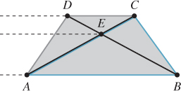
Figure 15.13: E is the centroid of square ABCD in 3D, but its projection is not the centroid of the projection of the square. This can be seen from the fact that the three dashed lines are not evenly spaced in 2D.
Fortunately, there is an efficient analog to 2D linear interpolation for projected 3D linear interpolation. This is interchangeably called hyperbolic interpolation [Bli93], perspective-correct interpolation [OG97], and rational linear interpolation [Hec90].
The perspective-correct interpolation method is simple. We can express it intuitively as, for each scalar vertex attribute u, linearly interpolate both u′ = u/z and 1/z in screen space. At each pixel, recover the 3D linearly interpolated attribute value from these by u = u′/(1/z). See the following sidebar for a more formal explanation of why this works.
![]() Let u(x, y, z) be some scalar attribute (e.g., albedo, u texture coordinate) that varies linearly over the polygon. Two equivalent definitions may be more intuitive: (a) u is defined at vertices by specific values and varies by barycentric interpolation between them; (b) u has the form of a 3D plane equation, u(x, y, z) = ax + by + cz + d.
Let u(x, y, z) be some scalar attribute (e.g., albedo, u texture coordinate) that varies linearly over the polygon. Two equivalent definitions may be more intuitive: (a) u is defined at vertices by specific values and varies by barycentric interpolation between them; (b) u has the form of a 3D plane equation, u(x, y, z) = ax + by + cz + d.
When the polygon is projected into screen space by the transformation (x, y, z) ![]() (–x/z, –y/z, –1) for an image plane at z = –1, then the function –u(x, y, z)/z varies linearly in screen space. Instead of linear interpolation in screen space, we need to perform a kind of “hyperbolic interpolation” to correctly evaluate u as follows.
(–x/z, –y/z, –1) for an image plane at z = –1, then the function –u(x, y, z)/z varies linearly in screen space. Instead of linear interpolation in screen space, we need to perform a kind of “hyperbolic interpolation” to correctly evaluate u as follows.
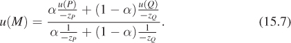
We can apply the perspective-correct interpolation strategy to any number of per-vertex attributes, including the vertex normals and texture coordinates. That leaves us with input data for our shade function, which remains unchanged from its implementation in the ray tracer.
15.6.4.3. 2D Barycentric Weights
To implement the perspective-correct interpolation strategy, we need only find an expression for the 2D barycentric weights at the center of each pixel. Consider the barycentric weight corresponding to vertex A of a point Q within a triangle ABC. Recall from Section 7.9 that this weight is the ratio of the distance from Q to the line containing BC to the distance from A to the line containing BC, that is, it is the relative distance across the triangle from the opposite edge. Listing 15.25 gives code for computing a barycentric weight in 2D.
Listing 15.25: Computing one barycentric weight in 2D.
1 /** Returns the distance from Q to the line containing B and A. */
2 float lineDistance2D(const Point2& A, const Point2& B, const Point2& Q) {
3 // Construct the line align:
4 const Vector2 n(A.y - B.y, B.x - A.x);
5 const float d = A.x * B.y - B.x * A.y;
6 return (n.dot(Q) + d) / n.length();
7 }
8
9 /** Returns the barycentric weight corresponding to vertex A of Q in triangle ABC */
10 float bary2D(const Point2& A, const Point2& B, const Point2& C, const Point2& Q) {
11 return lineDistance2D(B, C, Q) / lineDistance2D(B, C, A);
12 }
Under what condition could lineDistance2D return 0, or n.length() be 0, leading to a division by zero? Change your rasterizer to ensure that this condition never occurs. Why does this not affect the final rendering? What situation does this correspond to in a ray caster? How did we resolve that case when ray casting?
The rasterizer structure now requires a few changes from our previous version. It will need the post-projection vertices of the triangle after computing the bounding box in order to perform interpolation. We could either retain them from the bounding-box computation or just compute them again when needed later. We’ll recompute the values when needed because it trades a small amount of efficiency for a simpler interface to the bounding function, which makes the code easier to write and debug. Listing 15.26 shows the bounding box-function. The rasterizer must compute versions of the vertex attributes, which in our case are just the vertex normals, that are scaled by the ![]() value (which we call w) for the corresponding post-projective vertex. Both of those are per-triangle changes to the code. Finally, the inner loop must compute visibility from the 2D barycentric coordinates instead of from a ray cast. The actual shading computation remains unchanged from the original ray tracer, which is good—we’re only looking at strategies for visibility, not shading, so we’d like each to be as modular as possible. Listing 15.27 shows the loop setup of the original rasterizer updated with the bounding-box and 2D barycentric approach. Listing 15.28 shows how the inner loops change.
value (which we call w) for the corresponding post-projective vertex. Both of those are per-triangle changes to the code. Finally, the inner loop must compute visibility from the 2D barycentric coordinates instead of from a ray cast. The actual shading computation remains unchanged from the original ray tracer, which is good—we’re only looking at strategies for visibility, not shading, so we’d like each to be as modular as possible. Listing 15.27 shows the loop setup of the original rasterizer updated with the bounding-box and 2D barycentric approach. Listing 15.28 shows how the inner loops change.
Listing 15.26: Bounding box for the projection of a triangle, invoked by rasterize3 to establish the pixel iteration bounds.
1 void computeBoundingBox(const Triangle& T, const Camera& camera,
2 const Image& image,
3 Point2 V[3], int& x0, int& y0, int& x1, int& y1) {
4
5 Vector2 high(image.width(), image.height());
6 Vector2 low(0, 0);
7
8 for (int v = 0; v < 3; ++v) {
9 const Point2& X = perspectiveProject(T.vertex(v), image.width(),
10 image.height(), camera);
11 V[v] = X;
12 high = high.max(X);
13 low = low.min(X);
14 }
15
16 x0 = (int)floor(low.x);
17 x1 = (int)ceil(high.x);
18
19 y0 = (int)floor(low.y);
20 y1 = (int)ceil(high.y);
21 }
Listing 15.27: Iteration setup for a barycentric (edge align) rasterizer.
1 /** 2D barycentric evaluation w. perspective-correct attributes */
2 void rasterize3(Image& image, const Scene& scene,
3 const Camera& camera){
4 DepthBuffer depthBuffer(image.width(), image.height(), INFINITY);
5
6 // For each triangle
7 for (unsigned int t = 0; t < scene.triangleArray.size(); ++t) {
8 const Triangle& T = scene.triangleArray[t];
9
10 // Projected vertices
11 Vector2 V[3];
12 int x0, y0, x1, y1;
13 computeBoundingBox(T, camera, image, V, x0, y0, x1, y1);
14
15 // Vertex attributes, divided by -z
16 float vertexW[3];
17 Vector3 vertexNw[3];
18 Point3 vertexPw[3];
19 for (int v = 0; v < 3; ++v) {
20 const float w = -1.0f / T.vertex(v).z;
21 vertexW[v] = w;
22 vertexPw[v] = T.vertex(v) * w;
23 vertexNw[v] = T.normal(v) * w;
24 }
25
26 // For each pixel
27 for (int y = y0; y < y1; ++y) {
28 for (int x = x0; x < x1; ++x) {
29 // The pixel center
30 const Point2 Q(x + 0.5f, y + 0.5f);
31 . . .
32
33 }
34 }
35 }
36 }
Listing 15.28: Inner loop of a barycentric (edge align) rasterizer (see Listing 15.27 for the loop setup).
1 // For each pixel
2 for (int y = y0; y < y1; ++y) {
3 for (int x = x0; x < x1; ++x) {
4 // The pixel center
5 const Point2 Q(x + 0.5f, y + 0.5f);
6
7 // 2D Barycentric weights
8 const float weight2D[3] =
9 {bary2D(V[0], V[1], V[2], Q),
10 bary2D(V[1], V[2], V[0], Q),
11 bary2D(V[2], V[0], V[1], Q)};
12
13 if ((weight2D[0]>0) && (weight2D[1]>0) && (weight2D[2]>0)) {
14 // Interpolate depth
15 float w = 0.0f;
16 for (int v = 0; v < 3; ++v) {
17 w += weight2D[v] * vertexW[v];
18 }
19
20 // Interpolate projective attributes, e.g., P’, n’
21 Point3 Pw;
22 Vector3 nw;
23 for (int v = 0; v < 3; ++v) {
24 Pw += weight2D[v] * vertexPw[v];
25 nw += weight2D[v] * vertexNw[v];
26 }
27
28 // Recover interpolated 3D attributes; e.g., P’ -> P, n’ -> n
29 const Point3& P = Pw / w;
30 const Vector3& n = nw / w;
31
32 const float depth = P.length();
33 // We could also use depth = z-axis distance: depth = -P.z
34
35 // Depth test
36 if (depth < depthBuffer.get(x, y)) {
37 // Shade
38 Radiance3 L_o;
39 const Vector3& w_o = -P.direction();
40
41 // Make the surface normal have unit length
42 const Vector3& unitN = n.direction();
43 shade(scene, T, P, unitN, w_o, L_o);
44
45 depthBuffer.set(x, y, depth);
46 image.set(x, y, L_o);
47 }
48 }
49 }
50 }
To just test coverage, we don’t need the magnitude of the barycentric weights. We only need to know that they are all positive. That is, that the current sample is on the positive side of every line bounding the triangle. To perform that test, we could use the distance from a point to a line instead of the full bary2D result. For this reason, this approach to rasterization is also referred to as testing the edge aligns at each sample. Since we need the barycentric weights for interpolation anyway, it makes sense to normalize the distances where they are computed. Our first instinct is to delay that normalization at least until after we know that the pixel is going to be shaded. However, even for performance, that is unnecessary—if we’re going to optimize the inner loop, a much more significant optimization is available to us.
In general, barycentric weights vary linearly along any line through a triangle. The barycentric weight expressions are therefore linear in the loop variables x and y. You can see this by expanding bary2D in terms of the variables inside lineDistance2D, both from Listing 15.25. This becomes
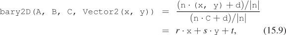
where the constants r, s, and t depend only on the triangle, and so are invariant across the triangle. We are particularly interested in properties invariant over horizontal and vertical lines, since those are our iteration directions.
For instance, y is invariant over the innermost loop along a scanline. Because the expressions inside the inner loop are constant in y (and all properties of T) and linear in x, we can compute them incrementally by accumulating derivatives with respect to x. That means that we can reduce all the computation inside the innermost loop and before the branch to three additions. Following the same argument for y, we can also reduce the computation that moves between rows to three additions. The only unavoidable operations are that for each sample that enters the branch for shading, we must perform three multiplications per scalar attribute; and we must perform a single division to compute z = –1/w, which is amortized over all attributes.
15.6.4.4. Precision for Incremental Interpolation
![]() We need to think carefully about precision when incrementally accumulating derivatives rather than explicitly performing linear interpolation by the barycentric coordinates. To ensure that rasterization produces complementary pixel coverage for adjacent triangles with shared vertices (“watertight rasterization”), we must ensure that both triangles accumulate the same barycentric values at the shared edge as they iterate across their different bounding boxes. This means that we need an exact representation of the barycentric derivative. To accomplish this, we must first round vertices to some imposed precision (say, one-quarter of a pixel width), and must then choose a representation and maximum screen size that provide exact storage.
We need to think carefully about precision when incrementally accumulating derivatives rather than explicitly performing linear interpolation by the barycentric coordinates. To ensure that rasterization produces complementary pixel coverage for adjacent triangles with shared vertices (“watertight rasterization”), we must ensure that both triangles accumulate the same barycentric values at the shared edge as they iterate across their different bounding boxes. This means that we need an exact representation of the barycentric derivative. To accomplish this, we must first round vertices to some imposed precision (say, one-quarter of a pixel width), and must then choose a representation and maximum screen size that provide exact storage.
The fundamental operation in the rasterizer is a 2D dot product to determine the side of the line on which a point lies. So we care about the precision of a multiplication and an addition. If our screen resolution is w × h and we want k × k subpixel positions for snapping or antialiasing, then we need ![]() log2(k·max(w, h))
log2(k·max(w, h))![]() bits to store each scalar value. At 1920 × 1080 (i.e., effectively 2048 × 2048) with 4 × 4 subpixel precision, that’s 14 bits. To store the product, we need twice as many bits. In our example, that’s 28 bits. This is too large for the 23-bit mantissa portion of the IEEE 754 32-bit floating-point format, which means that we cannot implement the rasterizer using the single-precision
bits to store each scalar value. At 1920 × 1080 (i.e., effectively 2048 × 2048) with 4 × 4 subpixel precision, that’s 14 bits. To store the product, we need twice as many bits. In our example, that’s 28 bits. This is too large for the 23-bit mantissa portion of the IEEE 754 32-bit floating-point format, which means that we cannot implement the rasterizer using the single-precision float data type. We can use a 32-bit integer, representing a 24.4 fixed-point value. In fact, within that integer’s space limitations we can increase screen resolution to 8192 × 8192 at 4 × 4 subpixel resolution. This is actually a fairly low-resolution subpixel grid, however. In contrast, DirectX 11 mandates eight bits of subpixel precision in each dimension. That is because under low subpixel precision, the aliasing pattern of a diagonal edge moving slowly across the screen appears to jump in discrete steps rather than evolve slowly with motion.
15.6.5. Rasterizing Shadows
Although we are now rasterizing primary visibility, our shade routine still determines the locations of shadows by casting rays. Shadowing from a local point source is equivalent to “visibility” from the perspective of that source. So we can apply rasterization to that visibility problem as well.
A shadow map [Wil78] is an auxiliary depth buffer rendered from a camera placed at the light’s location. This contains the same distance information as obtained by casting rays from the light to selected points in the scene. The shadow map can be rendered in one pass over the scene geometry before the camera’s view is rendered. Figure 15.14 shows a visualization of a shadow map, which is a common debugging aid.

Figure 15.14: Left: A shadow map visualized with black = near the light and white = far from the light. Right: The camera’s view of the scene with shadows.
When a shadowing computation arises during rendering from the camera’s view, the renderer uses the shadow map to resolve it. For a rendered point to be unshadowed, it must be simultaneously visible to both the light and the camera. Recall that we are assuming a pinhole camera and a point light source, so the paths from the point to each are defined by line segments of known length and orientation. Projecting the 3D point into the image space of the shadow map gives a 2D point. At that 2D point (or, more precisely, at a nearby one determined by rounding to the sampling grid for the shadow map) we previously stored the distance from the light to the first scene point, that is, the key information about the line segment. If that stored distance is equal to the distance from the 3D point to the 3D light source, then there must not have been any occluding surface and our point is lit. If the distance is less, then the point is in shadow because the light observes some other, shadow-casting, point first along the ray. This depth test must of course be conservative and approximate; we know there will be aliasing from both 2D discretization of the shadow map and its limited precision at each point.
Although we motivated shadow maps in the context of rasterization, they may be generated by or used to compute shadowing with both rasterization and ray casting renderers. There are often reasons to prefer to use the same visibility strategy throughout an application (e.g., the presence of efficient rasterization hardware), but there is no algorithmic constraint that we must do so.
When using a shadow map with triangle rasterization, we can amortize the cost of perspective projection into the shadow map over the triangle by performing most of the computational work at the vertices and then interpolating the results. The result must be interpolated in a perspective-correct fashion, of course. The key is that we want to be perspective-correct with respect to the matrix that maps points in world space to the shadow map, not to the viewport.
Recall the perspective-correct interpolation that we used for positions and texture coordinates (see previous sidebar, which essentially relied on linearly interpolating quantities of the form ![]() /z and w = –1/z). If we multiply world-space vertices by the matrix that transforms them into 2D shadow map coordinates but do not perform the homogeneous division, then we have a value that varies linearly in the homogeneous clip space of the virtual camera at the light that produces the shadow map. In other words, we project each vertex into both the viewing camera’s and the light camera’s homogeneous clip space. We next perform the homogeneous division for the visible camera only and interpolate the four-component homogeneous vector representing the shadow map coordinate in a perspective-correct fashion in screen space. We next perform the perspective division for the shadow map coordinate at each pixel, paying only for the division and not the matrix product at each pixel. This allows us to transform to the light’s projective view volume once per vertex and then interpolate those coordinates using the infrastructure already built for interpolating other elements. The reuse of a general interpolation mechanism and optimization of reducing transformations should naturally suggest that this approach is a good one for a hardware implementation of the graphics pipeline. Chapter 38 discusses how some of these ideas manifest in a particular graphics processor.
/z and w = –1/z). If we multiply world-space vertices by the matrix that transforms them into 2D shadow map coordinates but do not perform the homogeneous division, then we have a value that varies linearly in the homogeneous clip space of the virtual camera at the light that produces the shadow map. In other words, we project each vertex into both the viewing camera’s and the light camera’s homogeneous clip space. We next perform the homogeneous division for the visible camera only and interpolate the four-component homogeneous vector representing the shadow map coordinate in a perspective-correct fashion in screen space. We next perform the perspective division for the shadow map coordinate at each pixel, paying only for the division and not the matrix product at each pixel. This allows us to transform to the light’s projective view volume once per vertex and then interpolate those coordinates using the infrastructure already built for interpolating other elements. The reuse of a general interpolation mechanism and optimization of reducing transformations should naturally suggest that this approach is a good one for a hardware implementation of the graphics pipeline. Chapter 38 discusses how some of these ideas manifest in a particular graphics processor.
15.6.6. Beyond the Bounding Box
![]() A triangle touching Ο(n) pixels may have a bounding box containing Ο(n2) pixels. For triangles with all short edges, especially those with an area of about one pixel, rasterizing by iterating through all pixels in the bounding box is very efficient. Furthermore, the rasterization workload is very predictable for meshes of such triangles, since the number of tests to perform is immediately evident from the box bounds, and rectangular iteration is generally easier than triangular iteration.
A triangle touching Ο(n) pixels may have a bounding box containing Ο(n2) pixels. For triangles with all short edges, especially those with an area of about one pixel, rasterizing by iterating through all pixels in the bounding box is very efficient. Furthermore, the rasterization workload is very predictable for meshes of such triangles, since the number of tests to perform is immediately evident from the box bounds, and rectangular iteration is generally easier than triangular iteration.
For triangles with some large edges, iterating over the bounding box is a poor strategy because n2 ![]() n for large n. In this case, other strategies can be more efficient. We now describe some of these briefly. Although we will not explore these strategies further, they make great projects for learning about hardware-aware algorithms and primary visibility computation.
n for large n. In this case, other strategies can be more efficient. We now describe some of these briefly. Although we will not explore these strategies further, they make great projects for learning about hardware-aware algorithms and primary visibility computation.
15.6.6.1. Hierarchical Rasterization
Since the bounding-box rasterizer is efficient for small triangles and is easy to implement, a natural algorithmic approach is to recursively apply the bounding-box algorithm at increasingly fine resolution. This strategy is called hierarchical rasterization [Gre96].
Begin by dividing the entire image along a very coarse grid, such as into 16 × 16 macro-pixels that cover the entire screen. Apply a conservative variation of the bounding-box algorithm to these. Then subdivide the coarse grid and recursively apply the rasterization algorithm within all of the macro cells that overlapped the bounding box.
The algorithm could recur until the macro-pixels were actually a single pixel. However, at some point, we are able to perform a large number of tests either with Single Instruction Multiple Data (SIMD) operations or by using bitmasks packed into integers, so it may not always be a good idea to choose a single pixel as the base case. This is similar to the argument that you shouldn’t quicksort all the way down to a length 1 array; for small problem sizes, the constant factors affect the performance more than the asymptotic bound.
For a given precision, one can precompute all the possible ways that a line passes through a tile of samples. These can be stored as bitmasks and indexed by the line’s intercept points with the tile [FFR83, SW83]. For each line, using one bit to encode whether the sample is in the positive half-plane of the line allows an 8 × 8 pattern to fit in a single unsigned 64-bit integer. The bitwise AND of the patterns for the three line aligns defining the triangle gives the coverage mask for all 64 samples. One can use this trick to cull whole tiles efficiently, as well as avoiding per-sample visibility tests. (Kautz et al. [KLA04] extended this to a clever algorithm for rasterizing triangles onto hemispheres, which occurs frequently when sampling indirect illumination.) Furthermore, one can process multiple tiles simultaneously on a parallel processor. This is similar to the way that many GPUs rasterize today.
15.6.6.2. Chunking/Tiling Rasterization
A chunking rasterizer, a.k.a. a tiling rasterizer, subdivides the image into rectangular tiles, as if performing the first iteration of hierarchical rasterization. Instead of rasterizing a single triangle and performing recursive subdivision of the image, it takes all triangles in the scene and bins them according to which tiles they touch. A single triangle may appear in multiple bins.
The tiling rasterizer then uses some other method to rasterize within each tile. One good choice is to make the tiles 8 × 8 or some other size at which brute-force SIMD rasterization by a lookup table is feasible.
Working with small areas of the screen is a way to combine some of the best aspects of rasterization and ray casting. It maintains both triangle list and buffer memory coherence. It also allows triangle-level sorting so that visibility can be performed analytically instead of using a depth buffer. That allows both more efficient visibility algorithms and the opportunity to handle translucent surfaces in more sophisticated ways.
15.6.6.3. Incremental Scanline Rasterization
For each row of pixels within the bounding box, there is some location that begins the span of pixels covered by the triangle and some location that ends the span. The bounding box contains the triangle vertically and triangles are convex, so there is exactly one span per row (although if the span is small, it may not actually cover the center of any pixels).
A scanline rasterizer divides the triangle into two triangles that meet at a horizontal line through the vertex with the median vertical ordinate of the original triangle (see Figure 15.15). One of these triangles may have zero area, since the original triangle may contain a horizontal edge.
The scanline rasterizer computes the rational slopes of the left and right edges of the top triangle. It then iterates down these in parallel (see Figure 15.16). Since these edges bound the beginning and end of the span across each scan-line, no explicit per-pixel sample tests are needed: Every pixel center between the left and right edges at a given scanline is covered by the triangle. The rasterizer then iterates up the bottom triangle from the bottom vertex in the same fashion. Alternatively, it can iterate down the edges of the bottom triangle toward that vertex.
Figure 15.16: Each span’s starting point shifts Δ1 from that of the previous span, and its ending point shifts Δ2.
The process of iterating along an edge is performed by a variant of either the Digital Difference Analyzer (DDA) or Bresenham line algorithm [Bre65], for which there are efficient floating-point and fixed-point implementations.
Pineda [Pin88] discusses several methods for altering the iteration pattern to maximize memory coherence. On current processor architectures this approach is generally eschewed in favor of tiled rasterization because it is hard to schedule for coherent parallel execution and frequently yields poor cache behavior.
15.6.6.4. Micropolygon Rasterization
Hierarchical rasterization recursively subdivided the image so that the triangle was always small relative to the number of macro-pixels in the image. An alternative is to maintain constant pixel size and instead subdivide the triangle. For example, each triangle can be divided into four similar triangles (see Figure 15.17). This is the rasterization strategy of the Reyes system [CCC87] used in one of the most popular film renderers, RenderMan. The subdivision process continues until the triangles cover about one pixel each. These triangles are called micropolygons. In addition to triangles, the algorithm is often applied to bilinear patches, that is, Bézier surfaces described by four control points (see Chapter 23).
Subdividing the geometry offers several advantages over subdividing the image. It allows additional geometric processing, such as displacement mapping, to be applied to the vertices after subdivision. This ensures that displacement is performed at (or slightly higher than) image resolution, effectively producing perfect level of detail. Shading can be performed at vertices of the micropolygons and interpolated to pixel centers. This means that the shading is “attached” to object-space locations instead of screen-space locations. This can cause shading features, such as highlights and edges, which move as the surface animates, to move more smoothly and with less aliasing than they do when we use screen-space shading. Finally, effects like motion blur and defocus can be applied by deforming the final shaded geometry before rasterization. This allows computation of shading at a rate proportional to visible geometric complexity but independent of temporal and lens sampling.
15.7. Rendering with a Rasterization API
Rasterization has been encapsulated in APIs. We’ve seen that although the basic rasterization algorithm is very simple, the process of increasing its performance can rapidly introduce complexity. Very-high-performance rasterizers can be very complex. This complexity leads to a desire to separate out the parts of the rasterizer that we might wish to change between applications while encapsulating the parts that we would like to optimize once, abstract with an API, and then never change again. Of course, it is rare that one truly is willing to never alter an algorithm again, so this means that by building an API for part of the rasterizer we are trading performance and ease of use in some cases for flexibility in others. Hardware rasterizers are an extreme example of an optimized implementation, where flexibility is severely compromised in exchange for very high performance.
There have been several popular rasterization APIs. Today, OpenGL and DirectX are among the most popular hardware APIs for real-time applications. RenderMan is a popular software rasterization API for offline rendering. The space in between, of software rasterizers that run in real time on GPUs, is currently a popular research area with a few open source implementations available [LHLW10, LK11, Pan11].
In contrast to the relative standardization and popularity enjoyed among rasterizer APIs, several ray-casting systems have been built and several APIs have been proposed, although they have yet to reach the current level of standardization and acceptance of the rasterization APIs.
This section describes the OpenGL-DirectX abstraction in general terms. We prefer generalities because the exact entry points for these APIs change on a fairly regular basis. The details of the current versions can be found in their respective manuals. While important for implementation, those details obscure the important ideas.
15.7.1. The Graphics Pipeline
Consider the basic operations of any of our software rasterizer implementations:
1. (Vertex) Per-vertex transformation to screen space
2. (Rasterize) Per-triangle (clipping to the near plane and) iteration over pixels, with perspective-correct interpolation
3. (Pixel) Per-pixel shading
4. (Output Merge) Merging the output of shading with the current color and depth buffers (e.g., alpha blending)
These are the major stages of a rasterization API, and they form a sequence called the graphics pipeline, which was introduced in Chapter 1. Throughout the rest of this chapter, we refer to software that invokes API entry points as host code and software that is invoked as callbacks by the API as device code. In the context of a hardware-accelerated implementation, such as OpenGL on a GPU, this means that the C++ code running on the CPU is host code and the vertex and pixel shaders executing on the GPU are device code.
15.7.1.1. Rasterizing Stage
Most of the complexity that we would like such an API to abstract is in the rasterizing stage. Under current algorithms, rasterization is most efficient when implemented with only a few parameters, so this stage is usually implemented as a fixed-function unit. In hardware this may literally mean a specific circuit that can only compute rasterization. In software this may simply denote a module that accepts no parameterization.
15.7.1.2. Vertex and Pixel Stages
The per-vertex and per-pixel operations are ones for which a programmer using the API may need to perform a great deal of customization to produce the desired image. For example, an engineering application may require an orthographic projection of each vertex instead of a perspective one. We’ve already changed our per-pixel shading code three times, to support Lambertian, Blinn-Phong, and Blinn-Phong plus shadowing, so clearly customization of that stage is important. The performance impact of allowing nearly unlimited customization of vertex and pixel operations is relatively small compared to the benefits of that customization and the cost of rasterization and output merging. Most APIs enable customization of vertex and pixel stages by accepting callback functions that are executed for each vertex and each pixel. In this case, the stages are called programmable units.
A pipeline implementation with programmable units is sometimes called a programmable pipeline. Beware that in this context, the pipeline order is in fact fixed, and only the units within it are programmable. Truly programmable pipelines in which the order of stages can be altered have been proposed [SFB+09] but are not currently in common use.
For historical reasons, the callback functions are often called shaders or programs. Thus, a pixel shader or “pixel program” is a callback function that will be executed at the per-pixel stage. For triangle rasterization, the pixel stage is often referred to as the fragment stage. A fragment is the portion of a triangle that overlaps the bounds of a pixel. It is a matter of viewpoint whether one is computing the shade of the fragment and sampling that shade at the pixel, or directly computing the shade at the pixel. The distinction only becomes important when computing visibility independently from shading. Multi-sample anti-aliasing (MSAA) is an example of this. Under that rasterization strategy, many visibility samples (with corresponding depth buffer and radiance samples) are computed within each pixel, but a single shade is applied to all the samples that pass the depth and visibility test. In this case, one truly is shading a fragment and not a pixel.
15.7.1.3. Output Merging Stage
The output merging stage is one that we might like to customize as consumers of the API. For example, one might imagine simulating translucent surfaces by blending the current and previous radiance values in the frame buffer. However, the output merger is also a stage that requires synchronization between potentially parallel instances of the pixel shading units, since it writes to a shared frame buffer. As a result, most APIs provide only limited customization at the output merge stage. That allows lockless access to the underlying data structures, since the implementation may explicitly schedule pixel shading to avoid contention at the frame buffer. The limited customization options typically allow the programmer to choose the operator for the depth comparison. They also typically allow a choice of compositing operator for color limited to linear blending, minimum, and maximum operations on the color values.
There are of course more operations for which one might wish to provide an abstracted interface. These include per-object and per-mesh transformations, tessellation of curved patches into triangles, and per-triangle operations like silhouette detection or surface extrusion. Various APIs offer abstractions of these within a programming model similar to vertex and pixel shaders.
Chapter 38 discusses how GPUs are designed to execute this pipeline efficiently. Also refer to your API manual for a discussion of the additional stages (e.g., tessellate, geometry) that may be available.
15.7.2. Interface
The interface to a software rasterization API can be very simple. Because a software rasterizer uses the same memory space and execution model as the host program, one can pass the scene as a pointer and the callbacks as function pointers or classes with virtual methods. Rather than individual triangles, it is convenient to pass whole meshes to a software rasterizer to decrease the per-triangle overhead.
For a hardware rasterization API, the host machine (i.e., CPU) and graphics device (i.e., GPU) may have separate memory spaces and execution models. In this case, shared memory and function pointers no longer suffice. Hardware rasterization APIs therefore must impose an explicit memory boundary and narrow entry points for negotiating it. (This is also true of the fallback and reference software implementations of those APIs, such as Mesa and DXRefRast.) Such an API requires the following entry points, which are detailed in subsequent subsections.
1. Allocate device memory.
2. Copy data between host and device memory.
3. Free device memory.
4. Load (and compile) a shading program from source.
5. Configure the output merger and other fixed-function state.
6. Bind a shading program and set its arguments.
7. Launch a draw call, a set of device threads to render a triangle list.
15.7.2.1. Memory Principles
![]() The memory management routines are conceptually straightforward. They correspond to
The memory management routines are conceptually straightforward. They correspond to malloc, memcpy, and free, and they are typically applied to large arrays, such as an array of vertex data. They are complicated by the details necessary to achieve high performance for the case where data must be transferred per rendered frame, rather than once per scene. This occurs when streaming geometry for a scene that is too large for the device memory; for example, in a world large enough that the viewer can only ever observe a small fraction at a time. It also occurs when a data stream from another device, such as a camera, is an input to the rendering algorithm. Furthermore, hybrid software-hardware rendering and physics algorithms perform some processing on each of the host and device and must communicate each frame.
One complicating factor for memory transfer is that it is often desirable to adjust the data layout and precision of arrays during the transfer. The data structure for 2D buffers such as images and depth buffers on the host often resembles the “linear,” row-major ordering that we have used in this chapter. On a graphics processor, 2D buffers are often wrapped along Hilbert or Z-shaped (Morton) curves, or at least grouped into small blocks that are themselves row-major (i.e., “block-linear”), to avoid the cache penalty of vertical iteration. The origin of a buffer may differ, and often additional padding is required to ensure that rows have specific memory alignments for wide vector operations and reduced pointer size.
Another complicating factor for memory transfer is that one would often like to overlap computation with memory operations to avoid stalling either the host or device. Asynchronous transfers are typically accomplished by semantically mapping device memory into the host address space. Regular host memory operations can then be performed as if both shared a memory space. In this case the programmer must manually synchronize both host and device programs to ensure that data is never read by one while being written by the other. Mapped memory is typically uncached and often has alignment considerations, so the programmer must furthermore be careful to control access patterns.
Note that memory transfers are intended for large data. For small values, such as scalars, 4×4 matrices, and even short arrays, it would be burdensome to explicitly allocate, copy, and free the values. For a shading program with twenty or so arguments, that would incur both runtime and software management overhead. So small values are often passed through a different API associated with shaders.
15.7.2.2. Memory Practice
Listing 15.30 shows part of an implementation of a triangle mesh class. Making rendering calls to transfer individual triangles from the host to the graphics device would be inefficient. So, the API forces us to load a large array of the geometry to the device once when the scene is created, and to encode that geometry as efficiently as possible.
Few programmers write directly to hardware graphics APIs. Those APIs reflect the fact that they are designed by committees and negotiated among vendors. They provide the necessary functionality but do so through awkward interfaces that obscure the underlying function of the calling code. Usage is error-prone because the code operates directly on pointers and uses manually managed memory.
For example, in OpenGL, the code to allocate a device array and bind it to a shader input looks something like Listing 15.29. Most programmers abstract these direct host calls into a vendor-independent, easier-to-use interface.
Listing 15.29: Host code for transferring an array of vertices to the device and binding it to a shader input.
1 // Allocate memory:
2 GLuint vbo;
3 glGenBuffers(1, &vbo);
4 glBindBuffer(GL_ARRAY_BUFFER, vbo);
5 glBufferData(GL_ARRAY_BUFFER, hostVertex.size() * 2 * sizeof(Vector3), NULL,GL_STATIC_DRAW);
6 GLvoid* deviceVertex = 0;
7 GLvoid* deviceNormal = hostVertex.size() * sizeof(Vector3);
8
9 // Copy memory:
10 glBufferSubData(GL_ARRAY_BUFFER, deviceVertex, hostVertex.size() *
sizeof(Point3), &hostVertex[0]);
11
12 // Bind the array to a shader input:
13 int vertexIndex = glGetAttribLocation(shader, "vertex");
14 glEnableVertexAttribArray(vertexIndex);
15 glVertexAttribPointer(vertexIndex, 3, GL_FLOAT, GL_FALSE, 0, deviceVertex);
Most programmers wrap the underlying hardware API with their own layer that is easier to use and provides type safety and memory management. This also has the advantage of abstracting the renderer from the specific hardware API. Most console, OS, and mobile device vendors intentionally use equivalent but incompatible hardware rendering APIs. Abstracting the specific hardware API into a generic one makes it easier for a single code base to support multiple platforms, albeit at the cost of one additional level of function invocation.
For Listing 15.30, we wrote to one such platform abstraction instead of directly to a hardware API. In this code, the VertexBuffer class is a managed memory array in device RAM and AttributeArray and IndexArray are subsets of a VertexBuffer. The “vertex” in the name means that these classes store per-vertex data. It does not mean that they store only vertex positions—for example, the m_normal array is stored in an AttributeArray. This naming convention is a bit confusing, but it is inherited from OpenGL and DirectX. You can either translate this code to the hardware API of your choice, implement the VertexBuffer and AttributeArray classes yourself, or use a higher-level API such as G3D that provides these abstractions.
Listing 15.30: Host code for an indexed triangle mesh (equivalent to a set of Triangle instances that share a BSDF).
1 class Mesh {
2 private:
3 AttributeArray m_vertex;
4 AttributeArray m_normal;
5 IndexStream m_index;
6
7 shared_ptr<BSDF> m_bsdf;
8
9 public:
10
11 Mesh() {}
12
13 Mesh(const std::vector<Point3>& vertex,
14 const std::vector<Vector3>& normal,
15 const std::vector<int>& index, const shared_ptr<BSDF>& bsdf) : m_bsdf(bsdf) {
16
17 shared_ptr<VertexBuffer> dataBuffer =
18 VertexBuffer::create((vertex.size() + normal.size()) *
19 sizeof(Vector3) + sizeof(int) * index.size());
20 m_vertex = AttributeArray(&vertex[0], vertex.size(), dataBuffer);
21 m_normal = AttributeArray(&normal[0], normal.size(), dataBuffer);
22
23 m_index = IndexStream(&index[0], index.size(), dataBuffer);
24 }
25
26 . . .
27 };
28
29 /** The rendering API pushes us towards a mesh representation
30 because it would be inefficient to make per-triangle calls. */
31 class MeshScene {
32 public:
33 std::vector<Light> lightArray;
34 std::vector<Mesh> meshArray;
35 };
Listing 15.31 shows how this code is used to model the triangle-and-ground-plane scene. In it, the process of uploading the geometry to the graphics device is entirely abstracted within the Mesh class.
Listing 15.31: Host code to create indexed triangle meshes for the triangle-plus-ground scene.
1 void makeTrianglePlusGroundScene(MeshScene& s) {
2 std::vector<Vector3> vertex, normal;
3 std::vector<int> index;
4
5 // Green triangle geometry
6 vertex.push_back(Point3(0,1,-2)); vertex.push_back(Point3(-1.9f,-1,-2));
vertex.push_back(Point3(1.6f,-0.5f,-2));
7 normal.push_back(Vector3(0,0.6f,1).direction()); normal.
push_back(Vector3(-0.4f,-0.4f, 1.0f).direction()); normal.
push_back(Vector3(0.4f,-0.4f, 1.0f).direction());
8 index.push_back(0); index.push_back(1); index.push_back(2);
9 index.push_back(0); index.push_back(2); index.push_back(1);
10 shared_ptr<BSDF> greenBSDF(new PhongBSDF(Color3::green() * 0.8f,
11 Color3::white() * 0.2f, 100));
12
13 s.meshArray.push_back(Mesh(vertex, normal, index, greenBSDF));
14 vertex.clear(); normal.clear(); index.clear();
15
16 /////////////////////////////////////////////////////////
17 // Ground plane geometry
18 const float groundY = -1.0f;
19 vertex.push_back(Point3(-10, groundY, -10)); vertex.push_back(Point3(-10,
20 groundY, -0.01f));
21 vertex.push_back(Point3(10, groundY, -0.01f)); vertex.push_back(Point3(10,
22 groundY, -10));
23
24 normal.push_back(Vector3::unitY()); normal.push_back(Vector3::unitY());
25 normal.push_back(Vector3::unitY()); normal.push_back(Vector3::unitY());
26
27 index.push_back(0); index.push_back(1); index.push_back(2);
28 index.push_back(0); index.push_back(2); index.push_back(3);
29
30 const Color3 groundColor = Color3::white() * 0.8f;
31 s.meshArray.push_back(Mesh(vertex, normal, index, groundColor));
32
33 //////////////////////////////////////////////////////////
34 // Light source
35 s.lightArray.resize(1);
36 s.lightArray[0].position = Vector3(1, 3, 1);
37 s.lightArray[0].power = Color3::white() * 31.0f;
38 }
15.7.2.3. Creating Shaders
The vertex shader must transform the input vertex in global coordinates to a homogeneous point on the image plane. Listing 15.32 implements this transformation. We chose to use the OpenGL Shading Language (GLSL). GLSL is representative of other contemporary shading languages like HLSL, Cg, and RenderMan. All of these are similar to C++. However, there are some minor syntactic differences between GLSL and C++ that we call out here to aid your reading of this example. In GLSL,
• Arguments that are constant over all triangles are passed as global (“uniform”) variables.
• Points, vectors, and colors are all stored in vec3 type.
• const has different semantics (compile-time constant).
• in, out, and inout are used in place of C++ reference syntax.
• length, dot, etc. are functions instead of methods on vector classes.
Listing 15.32: Vertex shader for projecting vertices. The output is in homogeneous space before the division operation. This corresponds to the perspectiveProject function from Listing 15.24.
1 #version 130
2
3 // Triangle vertices
4 in vec3 vertex;
5 in vec3 normal;
6
7 // Camera and screen parameters
8 uniform float fieldOfViewX;
9 uniform float zNear;
10 uniform float zFar;
11 uniform float width;
12 uniform float height;
13
14 // Position to be interpolated
15 out vec3 Pinterp;
16
17 // Normal to be interpolated
18 out vec3 ninterp;
19
20 vec4 perspectiveProject(in vec3 P) {
21 // Compute the side of a square at z = -1 based on our
22 // horizontal left-edge-to-right-edge field of view .
23 float s = -2.0f * tan(fieldOfViewX * 0.5f);
24 float aspect = height / width;
25
26 // Project onto z = -1
27 vec4 Q;
28 Q.x = 2.0 * -Q.x / s;
29 Q.y = 2.0 * -Q.y / (s * aspect);
30 Q.z = 1.0;
31 Q.w = -P.z;
32
33 return Q;
34 }
35
36 void main() {
37 Pinterp = vertex;
38 ninterp = normal;
39
40 gl_Position = perspectiveProject(Pinterp);
41 }
None of these affect the expressiveness or performance of the basic language. The specifics of shading-language syntax change frequently as new versions are released, so don’t focus too much on the details. The point of this example is how the overall form of our original program is preserved but adjusted to the conventions of the hardware API.
Under the OpenGL API, the outputs of a vertex shader are a set of attributes and a vertex of the form (x, y, a, –z). That is, a homogeneous point for which the perspective division has not yet been performed. The value a/– z will be used for the depth test. We choose a = 1 so that the depth test is performed on –1/z, which is a positive value for the negative z locations that will be visible to the camera. We previously saw that any function that provides a consistent depth ordering can be used for the depth test. We mentioned that distance along the eye ray, –z, and –1/z are common choices. Typically one scales the a value such that –a/z is in the range [0, 1] or [–1, 1], but for simplicity we’ll omit that here. See Chapter 13 for the derivation of that transformation.
Note that we did not scale the output vertex to the dimensions of the image, negate the y-axis, or translate the origin to the upper left in screen space, as we did for the software renderer. That is because by convention, OpenGL considers the upper-left corner of the screen to be at (–1, 1) and the lower-right corner at (1, –1).
We choose the 3D position of the vertex and its normal as our attributes. The hardware rasterizer will automatically interpolate these across the surface of the triangle in a perspective-correct manner. We need to treat the vertex as an attribute because OpenGL does not expose the 3D coordinates of the point being shaded.
Listings 15.33 and 15.34 give the pixel shader code for the shade routine, which corresponds to the shade function from Listing 15.17, and helper functions that correspond to the visible and BSDF::evaluateFiniteScatteringDensity routines from the ray tracer and software rasterizer. The output of the shader is in homogeneous space before the division operation. This corresponds to the perspectiveProject function from Listing 15.24. The interpolated attributes enter the shader as global variables Pinterp and ninterp. We then perform shading in exactly the same manner as for the software renderers.
Listing 15.33: Pixel shader for computing the radiance scattered toward the camera from one triangle illuminated by one light.
1 #version 130
2 // BSDF
3 uniform vec3 lambertian;
4 uniform vec3 glossy;
5 uniform float glossySharpness;
6
7 // Light
8 uniform vec3 lightPosition;
9 uniform vec3 lightPower;
10
11 // Pre-rendered depth map from the light’s position
12 uniform sampler2DShadow shadowMap;
13
14 // Point being shaded. OpenGL has automatically performed
15 // homogeneous division and perspective-correct interpolation for us.
16 in vec3 Pinterp;
17 in vec3 ninterp;
18
19 // Value we are computing
20 out vec3 radiance;
21
22 // Normalize the interpolated normal; OpenGL does not automatically
23 // renormalize for us.
24 vec3 n = normalize(ninterp);
25
26 vec3 shade(const in vec3 P, const in vec3 n) {
27 vec3 radiance = vec3(0.0);
28
29 // Assume only one light
30 vec3 offset = lightPosition - P;
31 float distanceToLight = length(offset);
32 vec3 w_i = offset / distanceToLight;
33 vec3 w_o = -normalize(P);
34
35 if (visible(P, w_i, distanceToLight, shadowMap)) {
36 vec3 L_i = lightPower / (4 * PI * distanceToLight * distanceToLight);
37
38 // Scatter the light.
39 radiance +=
40 L_i *
41 evaluateFiniteScatteringDensity(w_i, w_o) *
42 max(0.0, dot(w_i, n));
43 }
44
45 return radiance;
46 }
47
48 void main() {
49 vec3 P = Pinterp;
50
51
52 radiance = shade(P, n);
53 }
Listing 15.34: Helper functions for the pixel shader.
1 #define PI 3.1415927
2
3 bool visible(const in vec3 P, const in vec3 w_i, const in float distanceToLight,
sampler2DShadow shadowMap) {
4 return true;
5 }
6
7 /** Returns f(wi, wo). Same as BSDF::evaluateFiniteScatteringDensity
8 from the ray tracer. */
9 vec3 evaluateFiniteScatteringDensity(const in vec3 w_i, const in vec3 w_o) {
10 vec3 w_h = normalize(w_i + w_o);
11
12 return (k_L +
13 k_G * ((s + 8.0) * pow(max(0.0, dot(w_h, n)), s) / 8.0)) / PI;
14 }
However, there is one exception. The software renderers iterated over all the lights in the scene for each point to be shaded. The pixel shader is hardcoded to accept a single light source. That is because processing a variable number of arguments is challenging at the hardware level. For performance, the inputs to shaders are typically passed through registers, not heap memory. Register allocation is generally a major factor in optimization. Therefore, most shading compilers require the number of registers consumed to be known at compile time, which precludes passing variable length arrays. Programmers have developed three forward-rendering design patterns for working within this limitation. These use a single framebuffer and thus limit the total space required by the algorithm. A fourth and currently popular deferred-rendering method requires additional space.
1. Multipass Rendering: Make one pass per light over all geometry, summing the individual results. This works because light combines by superposition. However, one has to be careful to resolve visibility correctly on the first pass and then never alter the depth buffer. This is the simplest and most elegant solution. It is also the slowest because the overhead of launching a pixel shader may be significant, so launching it multiple times to shade the same point is inefficient.
2. Übershader: Bound the total number of lights, write a shader for that maximum number, and set the unused lights to have zero power. This is one of the most common solutions. If the overhead of launching the pixel shader is high and there is significant work involved in reading the BSDF parameters, the added cost of including a few unused lights may be low. This is a fairly straightforward modification to the base shader and is a good compromise between performance and code clarity.
3. Code Generation: Generate a set of shading programs, one for each number of lights. These are typically produced by writing another program that automatically generates the shader code. Load all of these shaders at runtime and bind whichever one matches the number of lights affecting a particular object. This achieves high performance if the shader only needs to be swapped a few times per frame, and is potentially the fastest method. However, it requires significant infrastructure for managing both the source code and the compiled versions of all the shaders, and may actually be slower than the conservative solution if changing shaders is an expensive operation.
If there are different BSDF terms for different surfaces, then we have to deal with all the permutations of the number of lights and the BSDF variations. We again choose between the above three options. This combinatorial explosion is one of the primary drawbacks of current shading languages, and it arises directly from the requirement that the shading compiler produce efficient code. It is not hard to design more flexible languages and to write compilers for them. But our motivation for moving to a hardware API was largely to achieve increased performance, so we are unlikely to accept a more general shading language if it significantly degrades performance.
4. Deferred Lighting: A deferred approach that addresses these problems but requires more memory is to separate the computation of which point will color each pixel from illumination computation. An initial rendering pass renders many parallel buffers that encode the shading coefficients, surface normal, and location of each point (often, assuming an übershader). Subsequent passes then iterate over the screen-space area conservatively affected by each light, computing and summing illumination. Two common structures for those lighting passes are multiple lights applied to large screen-space tiles and ellipsoids for individual lights that cover the volume within which their contribution is non-negligible.
For the single-light case, moving from our own software rasterizer to a hardware API did not change our perspectiveProject and shade functions substantially.
However, our shade function was not particularly powerful. Although we did not choose to do so, in our software rasterizer, we could have executed arbitrary code inside the shade function. For example, we could have written to locations other than the current pixel in the frame buffer, or cast rays for shadows or reflections. Such operations are typically disallowed in a hardware API. That is because they interfere with the implementation’s ability to efficiently schedule parallel instances of the shading programs in the absence of explicit (inefficient) memory locks.
This leaves us with two choices when designing an algorithm with more significant processing, especially at the pixel level. The first choice is to build a hybrid renderer that performs some of the processing on a more general processor, such as the host, or perhaps on a general computation API (e.g., CUDA, Direct Compute, OpenCL, OpenGL Compute). Hybrid renderers typically incur the cost of additional memory operations and the associated synchronization complexity.
The second choice is to frame the algorithm purely in terms of rasterization operations, and make multiple rasterization passes. For example, we can’t conveniently cast shadow rays in most hardware rendering APIs today. But we can sample from a previously rendered shadow map.
Similar methods exist for implementing reflection, refraction, and indirect illumination purely in terms of rasterization. These avoid much of the performance overhead of hybrid rendering and leverage the high performance of hardware rasterization. However, they may not be the most natural way of expressing an algorithm, and that may lead to a net inefficiency and certainly to additional software complexity. Recall that changing the order of iteration from ray casting to rasterization increased the space demands of rendering by requiring a depth buffer to store intermediate results. In general, converting an arbitrary algorithm to a rasterization-based one often has this effect. The space demands might grow larger than is practical in cases where those intermediate results are themselves large.
Shading languages are almost always compiled into executable code at runtime, inside the API. That is because even within products from one vendor the underlying micro-architecture may vary significantly. This creates a tension within the compiler between optimizing the target code and producing the executable quickly. Most implementations err on the side of optimization, since shaders are often loaded once per scene. Beware that if you synthesize or stream shaders throughout the rendering process there may be substantial overhead.
Some languages (e.g., HLSL and CUDA) offer an initial compilation step to an intermediate representation. This eliminates the runtime cost of parsing and some trivial compilation operations while maintaining flexibility to optimize for a specific device. It also allows software developers to distribute their graphics applications without revealing the shading programs to the end-user in a human-readable form on the file system. For closed systems with fixed specifications, such as game consoles, it is possible to compile shading programs down to true machine code. That is because on those systems the exact runtime device is known at host-program compile time. However, doing so would reveal some details of the proprietary micro-architecture, so even in this case vendors do not always choose to have their APIs perform a complete compilation step.
15.7.2.4. Executing Draw Calls
To invoke the shaders we issue draw calls. These occur on the host side. One typically clears the framebuffer, and then, for each mesh, performs the following operations.
1. Set fixed function state.
2. Bind a shader.
3. Set shader arguments.
4. Issue the draw call.
These are followed by a call to send the framebuffer to the display, which is often called a buffer swap. An abstracted implementation of this process might look like Listing 15.35. This is called from a main rendering loop, such as Listing 15.36.
Listing 15.35: Host code to set fixed-function state and shader arguments, and to launch a draw call under an abstracted hardware API.
1 void loopBody(RenderDevice* gpu) {
2 gpu->setColorClearValue(Color3::cyan() * 0.1f);
3 gpu->clear();
4
5 const Light& light = scene.lightArray[0];
6
7 for (unsigned int m = 0; m < scene.meshArray.size(); ++m) {
8 Args args;
9 const Mesh& mesh = scene.meshArray[m];
10 const shared_ptr<BSDF>& bsdf = mesh.bsdf();
11
12 args.setUniform("fieldOfViewX", camera.fieldOfViewX);
13 args.setUniform("zNear", camera.zNear);
14 args.setUniform("zFar", camera.zFar);
15
16 args.setUniform("lambertian", bsdf->lambertian);
17 args.setUniform("glossy", bsdf->glossy);
18 args.setUniform("glossySharpness", bsdf->glossySharpness);
19
20 args.setUniform("lightPosition", light.position);
21 args.setUniform("lightPower", light.power);
22
23 args.setUniform("shadowMap", shadowMap);
24
25 args.setUniform("width", gpu->width());
26 args.setUniform("height", gpu->height());
27
28 gpu->setShader(shader);
29
30 mesh.sendGeometry(gpu, args);
31 }
32 gpu->swapBuffers();
33 }
Listing 15.36: Host code to set up the main hardware rendering loop.
1 OSWindow::Settings osWindowSettings;
2 RenderDevice* gpu = new RenderDevice();
3 gpu->init(osWindowSettings);
4
5 // Load the vertex and pixel programs
6 shader = Shader::fromFiles("project.vrt", "shade.pix");
7
8 shadowMap = Texture::createEmpty("Shadow map", 1024, 1024,
9 ImageFormat::DEPTH24(), Texture::DIM_2D_NPOT, Texture::Settings::shadow());
10 makeTrianglePlusGroundScene(scene);
11
12 // The depth test will run directly on the interpolated value in
13 // Q.z/Q.w, which is going to be smallest at the far plane
14 gpu->setDepthTest(RenderDevice::DEPTH_GREATER);
15 gpu->setDepthClearValue(0.0);
16
17 while (! done) {
18 loopBody(gpu);
19 processUserInput();
20 }
21
22 ...
15.8. Performance and Optimization
We’ll now consider several examples of optimization in hardware-based rendering. This is by no means an exhaustive list, but rather a set of model techniques from which you can draw ideas to generate your own optimizations when you need them.
15.8.1. Abstraction Considerations
Many performance optimizations will come at the price of significantly complicating the implementation. Weigh the performance advantage of an optimization against the additional cost of debugging and code maintenance. High-level algorithmic optimizations may require significant thought and restructuring of code, but they tend to yield the best tradeoff of performance for code complexity. For example, simply dividing the screen in half and asynchronously rendering each side on a separate processor nearly doubles performance at the cost of perhaps 50 additional lines of code that do not interact with the inner loop of the renderer.
In contrast, consider some low-level optimizations that we intentionally passed over. These include reducing common subexpressions (e.g., mapping all of those repeated divisions to multiplications by an inverse that is computed once) and lifting constants outside loops. Performing those destroys the clarity of the algorithm, but will probably gain only a 50% throughput improvement.
This is not to say that low-level optimizations are not worthwhile. But they are primarily worthwhile when you have completed your high-level optimizations; at that point you are more willing to complicate your code and its maintenance because you are done adding features.
15.8.2. Architectural Considerations
![]() The primary difference between the simple rasterizer and ray caster described in this chapter is that the “for each pixel” and “for each triangle” loops have the opposite nesting. This is a trivial change and the body of the inner loop is largely similar in each case. But the trivial change has profound implications for memory access patterns and how we can algorithmically optimize each.
The primary difference between the simple rasterizer and ray caster described in this chapter is that the “for each pixel” and “for each triangle” loops have the opposite nesting. This is a trivial change and the body of the inner loop is largely similar in each case. But the trivial change has profound implications for memory access patterns and how we can algorithmically optimize each.
Scene triangles are typically stored in the heap. They may be in a flat 1D array, or arranged in a more sophisticated data structure. If they are in a simple data structure such as an array, then we can ensure reasonable memory coherence by iterating through them in the same order that they appear in memory. That produces efficient cache behavior. However, that iteration also requires substantial bandwidth because the entire scene will be processed for each pixel. If we use a more sophisticated data structure, then we likely will reduce bandwidth but also reduce memory coherence. Furthermore, adjacent pixels likely sample the same triangle, but by the time we have iterated through to testing that triangle again it is likely to have been flushed from the cache. A popular low-level optimization for a ray tracer is to trace a bundle of rays called a ray packet through adjacent pixels. These rays likely traverse the scene data structure in a similar way, which increases memory coherence. On a SIMD processor a single thread can trace an entire packet simultaneously. However, packet tracing suffers from computational coherence problems. Sometimes different rays in the same packet progress to different parts of the scene data structure or branch different ways in the ray intersection test. In these cases, processing multiple rays simultaneously on a thread gives no advantage because memory coherence is lost or both sides of the branch must be taken. As a result, fast ray tracers are often designed to trace packets through very sophisticated data structures. They are typically limited not by computation but by memory performance problems arising from resultant cache inefficiency.
Because frame buffer storage per pixel is often much smaller than scene structure per triangle, the rasterizer has an inherent memory performance advantage over the ray tracer. A rasterizer reads each triangle into memory and then processes it to completion, iterating over many pixels. Those pixels must be adjacent to each other in space. For a row-major image, if we iterate along rows, then the pixels covered by the triangle are also adjacent in memory and we will have excellent coherence and fairly low memory bandwidth in the inner loop. Furthermore, we can process multiple adjacent pixels, either horizontally or vertically, simultaneously on a SIMD architecture. These will be highly memory and branch coherent because we’re stepping along a single triangle. There are many variations on ray casting and rasterization that improve their asymptotic behavior. However, these algorithms have historically been applied to only millions of triangles and pixels. At those sizes, constant factors like coherence still drive the performance of the algorithms, and rasterization’s superior coherence properties have made it preferred for high-performance rendering. The cost of this coherence is that after even the few optimizations needed to get real-time performance from a rasterizer, the code becomes so littered with bit-manipulation tricks and highly derived terms that the elegance of a simple ray cast seems very attractive from a software engineering perspective. This difference is only magnified when we make the rendering algorithm more sophisticated. The conventional wisdom is that ray-tracing algorithms are elegant and easy to extend but are hard to optimize, and rasterization algorithms are very efficient but are awkward and hard to augment with new features. Of course, one can always make a ray tracer fast and ugly (which packet tracing succeeds at admirably) and a rasterizer extensible but slow (e.g., Pixar’s RenderMan, which was used extensively in film rendering over the past two decades).
15.8.3. Early-Depth-Test Example
One simple optimization that can significantly improve performance, yet only minimally affects clarity, is an early depth test. Both the rasterizer and the ray-tracer structures sometimes shaded a point, only to later find that some other point was closer to the surface. As an optimization, we might first find the closest point before doing any shading, then go back and shade the point that was closest. In ray tracing, each pixel is processed to completion before moving to the next, so this involves running the entire visibility loop for one pixel, maintaining the shading inputs for the closest-known intersection at each iteration, and then shading after that loop terminates. In rasterization, pixels are processed many times, so we have to make a complete first pass to determine visibility and then a second pass to do shading. This is called an early-depth pass [HW96] if it primes depthBuffer so that only the surface that shades will pass the inner test. The process is called deferred shading if it also accumulates the shading parameters so that they do not need to be recomputed. This style of rendering was first introduced by Whitted and Weimer [WW82] to compute shading independent from visibility at a time when primary visibility computation was considered expensive. Within a decade it was considered a method to accelerate complex rendering toward real-time rendering (and the “deferred” term was coined) [MEP92], and today its use is widespread as a further optimization on hardware platforms that already achieve real time for complex scenes.
For a scene that has high depth complexity (i.e., in which many triangles project to the same point in the image) and an expensive shading routine, the performance benefit of an early depth test is significant. The cost of rendering a pixel without an early depth test is Ο(tv + ts), where t is the number of triangles, v is the time for a visibility test, and s is the time for shading. This is an upper bound. When we are lucky and always encounter the closest triangle first, the performance matches the lower bound of Ω(tv + s) since we only shade once. The early-depth optimization ensures that we are always in this lower-bound case. We have seen how rasterization can drive the cost of v very low—it can be reduced to a few additions per pixel—at which point the challenge becomes reducing the number of triangles tested at each pixel. Unfortunately, that is not as simple. Strategies exist for obtaining expected Ο(v log t + s) rendering times for scenes with certain properties, but they significantly increase code complexity.
15.8.4. When Early Optimization Is Good
The domain of graphics raises two time-based exceptions to the general rule of thumb to avoid premature optimization. The more significant of these exceptions is that when low-level optimizations can accelerate a rendering algorithm just enough to make it run at interactive rates, it might be worth making those optimizations early in the development process. It is much easier to debug an interactive rendering system than an offline one. Interaction allows you to quickly experiment with new viewpoints and scene variations, effectively giving you a true 3D perception of your data instead of a 2D slice. If that lets you debug faster, then the optimization has increased your ability to work with the code despite the added complexity. The other exception applies when the render time is just at the threshold of your patience. Most programmers are willing to wait for 30 seconds for an image to render, but they will likely leave the computer or switch tasks if the render time is, say, more than two minutes. Every time you switch tasks or leave the computer you’re amplifying the time cost of debugging, because on your return you have to recall what you were doing before you left and get back into the development flow. If you can reduce the render time to something you are willing to wait for, then you have cut your debugging time and made the process sufficiently more pleasant that your productivity will again rise despite increased code complexity. We enshrine these ideas in a principle:
![]() The Early Optimization Principle
The Early Optimization Principle
It’s worth optimizing early if it makes the difference between an interactive program and one that takes several minutes to execute. Shortening the debugging cycle and supporting interactive testing are worth the extra effort.
15.8.5. Improving the Asymptotic Bound
To scale to truly large scenes, no linear-time rendering algorithm suffices. We must somehow eliminate whole parts of the scene without actually touching their data even once. Data structures for this are a classic area of computer graphics that continues to be a hot research topic. The basic idea behind most of these is the same as behind using tree and bucket data structures for search and sort problems. Visibility testing is primarily a search operation, where we are searching for the closest ray intersection with the scene. If we precompute a treelike data structure that orders the scene primitives in some way that allows conservatively culling a constant fraction of the primitives at each layer, we will approach Ο(log n)-time visibility testing for the entire scene, instead of Ο(n) in the number of primitives. When the cost of traversing tree nodes is sufficiently low, this strategy scales well for arbitrarily constructed scenes and allows an exponential increase in the number of primitives we can render in a fixed time. For scenes with specific kinds of structure we may be able to do even better. For example, say that we could find an indexing scheme or hash function that can divide our scene into Ο(n) buckets that allow conservative culling with Ο(1) primitives per bucket. This would approach Ο(d)-time visibility testing in the distance d to the first intersection. When that distance is small (e.g., in twisty corridors), the runtime of this scheme for static scenes becomes independent of the number of primitives and we can theoretically render arbitrarily large scenes. See Chapter 37 for a detailed discussion of algorithms based on these ideas.
15.9. Discussion
Our goal in this chapter was not to say, “You can build either a ray tracer or a rasterizer,” but rather that rendering involves sampling of light sources, objects, and rays, and that there are broad algorithmic strategies you can use for accumulating samples and interpolating among them. This provides a stage for all future rendering, where we try to select samples efficiently and with good statistical characteristics.
For sampling the scene along eye rays through pixel centers, we saw that three tests—explicit 3D ray-triangle tests, 2D ray-triangle through incremental barycentric tests, and 2D ray-triangle through incremental edge equation tests—were mathematically equivalent. We also discussed how to implement them so that the mathematical equivalence was preserved even in the context of bounded-precision arithmetic. In each case we computed some value directly related to the barycentric weights and then tested whether the weights corresponded to a point on the interior of the triangle. It is essential that these are mathematically equivalent tests. Were they not, we would not expect all methods to produce the same image! Algorithmically, these approaches led to very different strategies. That is because they allowed amortization in different ways and provoked different memory access patterns.
Sampling is the core of physically based rendering. The kinds of design choices you faced in this chapter echo throughout all aspects of rendering. In fact, they are significant for all high-performance computing, spreading into fields as diverse as biology, finance, and weather simulation. That is because many interesting problems do not admit analytic solutions and must be solved by taking discrete samples. One frequently wants to take many of those samples in parallel to reduce computation latency. So considerations about how to sample over a complex domain, which in our case was the set product of triangles and eye rays, are fundamental to science well beyond image synthesis.
The ray tracer in this chapter is a stripped-down, no-frills ray tracer. But it still works pretty well. Ten years ago you would have had to wait an hour for the teapot to render. It will probably take at most a few seconds on your computer today. This performance increase allows you to more freely experiment with the algorithms in this chapter than people have been able to in the past. It also allows you to exercise clearer software design and to quickly explore more sophisticated algorithms, since you need not spend significant time on low-level optimization to obtain reasonable rendering rates.
Despite the relatively high performance of modern machines, we still considered design choices and compromises related to the tension between abstraction and performance. That is because there are few places where that tension is felt as keenly in computer graphics as at the primary visibility level, and without at least some care our renderers would still have been unacceptably slow. This is largely because primary visibility is driven by large constants—scene complexity and the number of pixels—and because primary visibility is effectively the tail end of the graphics pipeline.
Someday, machines may be fast enough that we don’t have to make as many compromises to achieve acceptable rendering rates as we do today. For example, it would be desirable to operate at a purely algorithmic level without exposing the internal memory layout of our Image class. Whether this day arrives soon depends on both algorithmic and hardware advances. Previous hardware performance increases have in part been due to faster clock speeds and increased duplication of parallel processing and memory units. But today’s semiconductor-based processors are incapable of running at greater clock speeds because they have hit the limits of voltage leakage and inductive capacitance. So future speedups will not come from higher clock rates due to better manufacturing processes on the same substrates. Furthermore, the individual wires within today’s processors are close to one molecule in thickness, so we are near the limits of miniaturization for circuits. Many graphics algorithms are today limited by communication between parallel processing units and between memory and processors. That means that simply increasing the number of ALUs, lanes, or processing cores will not increase performance. In fact, increased parallelism can even decrease performance when runtime is dominated by communication. So we require radically new algorithms or hardware architectures, or much more sophisticated compilers, if we want today’s performance with better abstraction.
There are of course design considerations beyond sample statistics and raw efficiency. For example, we saw that if you’re sampling really small triangles, then micropolygons or tile rasterization seems like a good rendering strategy. However, what if you’re sampling shapes that aren’t triangles and can’t easily be subdivided? Shapes as simple as a sphere fall into this category. In that case, ray casting seems like a very good strategy because you can simply replace ray-triangle intersection with ray-sphere intersection. Any micro-optimization of a rasterizer must be evaluated compared to the question, “What if we could render one nontriangular shape, instead of thousands of small triangles?” At some point, the constants make working with more abstract models like spheres and spline surfaces more preferable than working with many triangles.
When we consider sampling visibility in not just space, but also exposure time and lens position, individual triangles become six-dimensional, nonpolyhedral shapes. While algorithms for rasterizing these have recently been developed, they are certainly more complicated than ray-sampling strategies. We’ve seen that small changes, such as inverting the order of two nested loops, can yield significant algorithmic implications. There are many such changes that one can make to visibility sampling strategies, and many that have been made previously. It is probably best to begin a renderer by considering the desired balance of performance and code manageability, the size of the triangles and target image, and the sampling patterns desired. One can then begin with the simplest visibility algorithm appropriate for those goals, and subsequently experiment with variations.
Many of these variations have already been tried and are discussed in the literature. Only a few of these are cited here. Appel presented the first significant 3D visibility solution of ray casting in 1968. Nearly half a century later, new sampling algorithms appear regularly in top publication venues and the industry is hard at work designing new hardware for visibility sampling. This means that the best strategies may still await discovery, so some of the variations you try should be of your own design!
15.10. Exercises
Exercise 15.1: Generalize the Image and DepthBuffer implementations into different instances of a single, templated buffer class.
Exercise 15.2: Use the equations from Section 7.8.2 to extend your ray tracer to also intersect spheres. A sphere does not define a barycentric coordinate frame or vertex normals. How will you compute the normal to the sphere?
Exercise 15.3: Expand the barycentric weight computation that is abstracted in the bary2D function so that it appears explicitly within the per-pixel loop. Then lift the computation of expressions that are constant along a row or column outside the corresponding loop. Your resultant code should contain a single division operation within the inner loop.
Exercise 15.4: Characterize the asymptotic performance of each algorithm described in Section 15.6. Under what circumstances would each algorithm be preferred, according to this analysis?
Exercise 15.5: Consider the “1D rasterization” problem of coloring the pixel centers (say, at integer locations) covered by a line segment lying on the real number line.
1. What is the longest a segment can be while covering no pixel centers? Draw the number line and it should be obvious.
2. If we rasterize by snapping vertices at real locations to the nearest integer locations, how does that affect your answer to the previous question?
(Hint: Nothing wider than 0.5 pixels can now hide between two pixel centers.)
3. If we rasterize in fixed point with 8-bit subpixel precision and snap vertices to that grid before rasterization, how does that affect your answer? (Hint: Pixel centers are now spaced every 256 units.)
Exercise 15.6: Say that we transform the final scene for our ray tracer by moving the teapot 10 cm and ground to the right by adding 10 cm to the x-ordinate of each vertex. We could also accomplish this by leaving the teapot in the original position and instead transforming the ray origins to the left by 10 cm. This is the Coordinate-System/Basis principle. Now, consider the case where we wish to render 1000 teapots with identical geometry but different positions and orientations. Describe how to modify your ray tracer to represent this scene without explicitly storing 1000 copies of the teapot geometry, and how to trace that scene representation. (This idea is called instancing.)
Exercise 15.7: One way to model scenes is with constructive solid geometry or CSG: building solid primitives like balls, filled cubes, etc., transformed and combined by boolean operations. For instance, one might take two unit spheres, one at the origin and one translated to (1. 7, 0, 0), and declare their intersection to be a “lens” shape, or their union to be a representation of a hydrogen molecule. If the shapes are defined by meshes representing their boundaries, finding a mesh representation of the union, intersection, or difference (everything in shape A that’s not in shape B) can be complex and costly. For ray casting, things are simpler.
(a) Show that if a and b are the intervals where the ray R intersects objects A and B, then a ∪ b is where R intersects A ∪ B; show similar statements for the intersection and difference.
(b) Suppose a CSG representation of a scene is described by a tree (where edges are transformations, leaves are primitives, and nodes are CSG operations like union, intersection, and difference); sketch a ray-intersect-CSG-tree algorithm. Note: Despite the simplicity of the ideas suggested in this exercise, the speedups offered by bounding-volume hierarchies described in Chapter 37 favor their use, at least for complex scenes.