
CHAPTER 2 Images and Imaging Operations
piˇx’eˇlla¯tėd a. picture broken into a regular tiling
piˇx’iˇlla¯tėd a. pixie-like, crazy, deranged
2.1 Introduction
This chapter focuses on images and simple image processing operations and is intended to lead to more advanced image analysis operations that can be used for machine vision in an industrial environment. Perhaps the main purpose of the chapter is to introduce the reader to some basic techniques and notation that will be of use throughout the book. However, the image processing algorithms introduced here are of value in their own right in disciplines ranging from remote sensing to medicine, and from forensic to military and scientific applications.
The images discussed in this chapter have already been obtained from suitable sensors: the sensors are covered in a later chapter. Typical of such images is that shown in Fig. 2.1a. This is a gray-tone image, which at first sight appears to be a normal “black and white” photograph. On closer inspection, however, it becomes clear that it is composed of a large number of individual picture cells, or pixels. In fact, the image is a 128 × 128 array of pixels. To get a better feel for the limitations of such a digitized image, Fig. 2.1b shows a section that has been enlarged so that the pixels can be examined individually. A threefold magnification factor has been used, and thus the visible part of Fig. 2.1b contains only a 42 × 42 array of pixels.
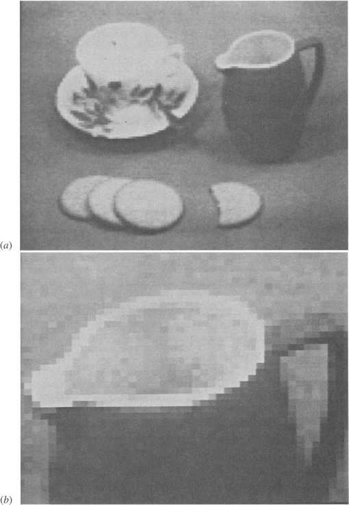
Figure 2.1 Typical gray-scale images: (a) gray-scale image digitized into a 128 × 128 array of pixels; (b) section of image shown in (a) subjected to threefold linear magnification: the individual pixels are now clearly visible.
It is not easy to see that these gray-tone images are digitized into a grayscale containing just 64 gray levels. To some extent, high spatial resolution compensates for the lack of gray-scale resolution, and as a result we cannot at once see the difference between an individual shade of gray and the shade it would have had in an ideal picture. In addition, when we look at the magnified section of image in Fig. 2.1b, it is difficult to understand the significance of the individual pixel intensities—the whole is becoming lost in a mass of small parts. Older television cameras typically gave a gray-scale resolution that was accurate only to about one part in 50, corresponding to about 6 bits of useful information per pixel. Modern solid-state cameras commonly give less noise and may allow 8 or even 9 bits of information per pixel. However, it is often not worthwhile to aim for such high gray-scale resolutions, particularly when the result will not be visible to the human eye, and when, for example, there is an enormous amount of other data that a robot can use to locate a particular object within the field of view. Note that if the human eye can see an object in a digitized image of particular spatial and gray-scale resolution, it is in principle possible to devise a computer algorithm to do the same thing.
Nevertheless, there is a range of applications for which it is valuable to retain good gray-scale resolution, so that highly accurate measurements can be made from a digital image. This is the case in many robotic applications, where high-accuracy checking of components is critical. More will be said about this subject later. In addition, in Part 2 we will see that certain techniques for locating components efficiently require that local edge orientation be estimated to better than 1°, and this can be achieved only if at least 6 bits of gray-scale information are available per pixel.
2.1.1 Gray-Scale versus Color
Returning now to the image of Fig. 2.1a, we might reasonably ask whether it would be better to replace the gray-scale with color, using an RGB (red, green, blue) color camera and three digitizers for the three main colors. Two aspects of color are important for the present discussion. One is the intrinsic value of color in machine vision: the other is the additional storage and processing penalty it might bring. It is tempting to say that the second aspect is of no great importance given the cheapness of modern computers which have both high storage and high speed. On the other hand, high-resolution images can arrive from a collection of CCTV cameras at huge data rates, and it will be many years before it will be possible to analyze all the data arriving from such sources. Hence, if color adds substantially to the storage and processing load, its use will need to be justified.
The potential of color in helping with many aspects of inspection, surveillance, control, and a wide variety of other applications including medicine (color plays a crucial role in images taken during surgery) is enormous. This potential is illustrated with regard to agriculture in Fig. 2.2; for robot navigation and driving in Figs. 2.3 and 2.4; for printed circuit board inspection in Fig. 2.5; for food inspection in Figs. 2.6 and 2.7; and for color filtering in Figs. 2.8 and 2.9. Notice that some of these images almost have color for color’s sake (especially in Figs. 2.6-2.8), though none of them is artificially generated. In others the color is more subdued (Figs. 2.2 and 2.4), and in Fig. 2.7 (excluding the tomatoes) it is quite subtle. The point here is that for color to be useful it need not be garish; it can be subtle as long as it brings the right sort of information to bear on the task in hand. Suffice it to say that in some of the simpler inspection applications, where mechanical components are scrutinized on a conveyor or workbench, it is quite likely the shape that is in question rather than the color of the object or its parts. On the other hand, if an automatic fruit picker is to be devised, it is much more likely to be crucial to check color rather than specific shape. We leave it to the reader to imagine when and where color is particularly useful or merely an unnecessary luxury.
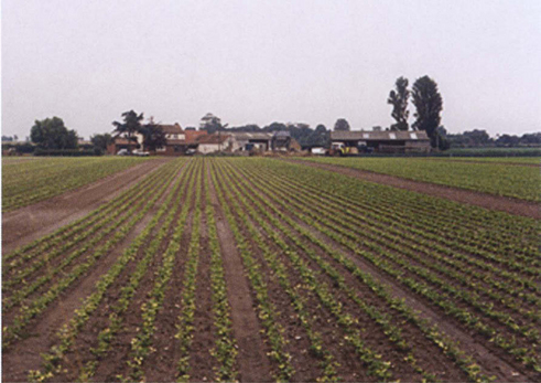
Figure 2.2 Value of color in agricultural applications. In agricultural scenes such as this one, color helps with segmentation and with recognition. It may be crucial in discriminating between weeds and crops if selective robot weedkilling is to be carried out. (See color insert.)
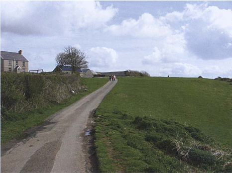
Figure 2.3 Value of color for segmentation and recognition. In natural outdoor scenes such as this one, color helps with segmentation and with recognition. While it may have been important to the early human when discerning sources of food in the wild, robot drones may benefit by using color to aid navigation. (See color insert.)
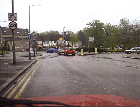
Figure 2.4 Value of color in the built environment. Color plays an important role for the human in managing the built environment. In a vehicle, a plethora of bright lights, road signs, and markings (such as yellow lines) are coded to help the driver. They may also help a robot to drive more safely by providing crucial information. (See color insert.)
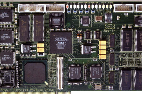
Figure 2.5 Value of color for unambiguous checking. In many inspection applications, color can be of help to unambiguously confirm the presence of certain objects, as on this printed circuit board. (See color insert.)
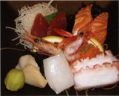
Figure 2.6 Value of color for food inspection. Much food is brightly colored, as with this Japanese meal. Although this may be attractive to the human, it could also help the robot to check quickly for foreign bodies or toxic substances. (See color insert.)
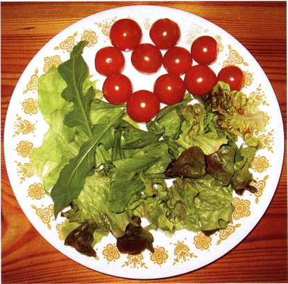
Figure 2.7 Subtle shades of color in food inspection. Although much food is brightly colored, as for the tomatoes in this picture, green salad leaves show much more subtle combinations of color and may indeed provide the only reliable means of identification. This could be important for inspection both of the raw product and its state when it reaches the warehouse or the supermarket. (See color insert.)
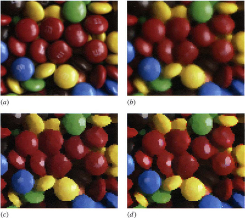
Figure 2.8 Color filtering of brightly colored objects. (a) Original color image of some sweets. (b) Vector median filtered version. (c) Vector mode filtered version. (d) Version to which a mode filter has been applied to each color channel separately. Note that (b) and (c) show no evidence of color bleeding, though it is strongly evident in (d). It is most noticeable as isolated pink pixels, plus a few green pixels, around the yellow sweets. For further details on color bleeding, see Section 3.14. (See color insert.)
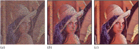
Figure 2.9 Color filtering of images containing substantial impulse noise. (a) Version of the Lena image containing 70% random color impulse noise. (b) Effect of applying a vector median filter, and (c) effect of applying a vector mode filter. Although the mode filter is designed more for enhancement than for noise suppression, it has been found to perform remarkably well at this task when the noise level is very high (see Section 3.4). (See color insert following p. 30)
Next, it is useful to consider the processing aspect of color. In many cases, good color discrimination is required to separate and segment two types of objects from each other. Typically, this will mean not using one or another specific color channel,1 but subtracting two, or combining three in such a way as to foster discrimination. In the worst case of combining three color channels by simple arithmetic processing in which each pixel is treated identically, the processing load will be very light. In contrast, the amount of processing required to determine the optimal means of combining the data from the color channels and to carry out different operations dynamically on different parts of the image may be far from negligible, and some care will be needed in the analysis. These problems arise because color signals are inhomogeneous. This contrasts with the situation for gray-scale images, where the bits representing the gray-scale are all of the same type and take the form of a number representing the pixel intensity: they can thus be processed as a single entity on a digital computer.
2.2 Image Processing Operations
The images of Figs 2.1 and 2.11a are considered in some detail here, including some of the many image processing operations that can be performed on them. The resolution of these images reveals a considerable amount of detail and at the same time shows how it relates to the more “meaningful” global information. This should help to show how simple imaging operations contribute to image interpretation.
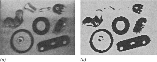
Figure 2.11 Thresholding of gray-scale images: (a) 128 × 128 pixel gray-scale image of a collection of parts; (b) effect of thresholding the image.
When performing image processing operations, we start with an image in one storage area and generate a new processed image in another storage area. In practice these storage areas may either be in a special hardware unit called a frame store that is interfaced to the computer, or else they may be in the main memory of the computer or on one of its discs. In the past, a special frame store was required to store images because each image contains a good fraction of a megabyte of information, and this amount of space was not available for normal users in the computer main memory. Today this is less of a problem, but for image acquisition a frame store is still required. However, we shall not worry about such details here; instead it will be assumed that all images are inherently visible and that they are stored in various image “spaces” P, Q, R, and so on. Thus, we might start with an image in space P and copy it to space Q, for example.
2.2.1 Some Basic Operations on Gray-scale Images
Perhaps the simplest imaging operation is that of clearing an image or setting the contents of a given image space to a constant level. We need some way of arranging this; accordingly, the following C++ routine may be written for implementing it:2
 (2.1)
(2.1)In this routine the local pixel intensity value is expressed as P[i][j], since P-space is taken to be a two-dimensional array of intensity values. In what follows it will be advantageous to rewrite such routines in the more succinct form:
since it is then much easier to understand the image processing operations. In effect, we are attempting to expose the fundamental imaging operation by removing irrelevant programming detail. The double square bracket notation is intended to show that the operation it encloses is applied at every pixel location in the image, for whatever size of image is currently defined. The reason for calling the pixel intensity P0 will become clear later.
Another simple imaging operation is to copy an image from one space to another. This is achieved, without changing the contents of the original space P, by the routine:
Again, the double bracket notation indicates a double loop that copies each individual pixel of P-space to the corresponding location in Q-space.
A more interesting operation is that of inverting the image, as in the process of converting a photographic negative to a positive. This process is represented as follows:
In this case it is assumed that pixel intensity values lie within the range 0-255, as is commonly true for frame stores that represent each pixel as one byte of information. Note that such intensity values are commonly unsigned, and this is assumed generally in what follows.
There are many operations of these types. Some other simple operations are those that shift the image left, right, up, down, or diagonally. They are easy to implement if the new local intensity is made identical to that at a neighboring location in the original image. It is evident how this would be expressed in the double suffix notation used in the original C++ routine. In the new shortened notation, it is necessary to name neighboring pixels in some convenient way, and we here employ a commonly used numbering scheme:

with a similar scheme for other image spaces. With this notation, it is easy to express a left shift of an image as follows:
Similarly, a shift down to the bottom right is expressed as:
(Note that the shift appears in a direction opposite to that which one might at first have suspected.)
It will now be clear why P0 and Q0 were chosen for the basic notation of pixel intensity: the “0” denotes the central pixel in the “neighborhood” or “window,” and corresponds to zero shift when copying from one space to another.
A whole range of possible operations is associated with modifying images in such a way as to make them more satisfactory for a human viewer. For example, adding a constant intensity makes the image brighter:
and the image can be made darker in the same way. A more interesting operation is to stretch the contrast of a dull image:
where gamma >1. In practice (as for Fig. 2.10) it is necessary to ensure that intensities do not result that are outside the normal range, for example, by using an operation of the form:
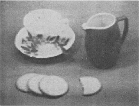
Figure 2.10 Contrast-stretching: effect of increasing the contrast in the image of Fig. 2.1a by a factor of two and adjusting the mean intensity level appropriately. The interior of the jug can now be seen more easily. Note, however, that there is no additional information in the new image.
 (2.9)
(2.9)Most practical situations demand more sophisticated transfer functions—either nonlinear or piecewise linear—but such complexities are ignored here.
A further simple operation that is often applied to gray-scale images is that of thresholding to convert to a binary image. This topic is covered in more detail later in this chapter since it is widely used to detect objects in images. However, our purpose here is to look on it as another basic imaging operation. It can be implemented using the routine3
If, as often happens, objects appear as dark objects on a light background, it is easier to visualize the subsequent binary processing operations by inverting the thresholded image using a routine such as
However, it would be more usual to combine the two operations into a single routine of the form:
To display the resulting image in a form as close as possible to the original, it can be reinverted and given the full range of intensity values (intensity values 0 and 1 being scarcely visible):
Figure 2.11 shows the effect of these two operations.
2.2.2 Basic Operations on Binary Images
Once the image has been thresholded, a wide range of binary imaging operations becomes possible. Only a few such operations are covered here, with the aim of being instructive rather than comprehensive. With this in mind, a routine may be written for shrinking dark thresholded objects (Fig. 2.12a), which are represented here by a set of 1’s in a background of 0’s:
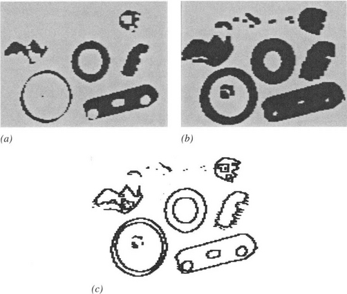
Figure 2.12 Simple operations applied to binary images: (a) effect of shrinking the dark-thresholded objects appearing in Fig. 2.11b; (b) effect of expanding these dark objects; (c) result of applying an edge location routine. Note that the SHRINK, EXPAND, and EDGE routines are applied to the dark objects. This implies that the intensities are initially inverted as part of the thresholding operation and then reinverted as part of the display operation (see text).
 (2.14)
In fact, the logic of this routine can be simplified to give the following more compact version:
Note that the process of shrinking4 dark objects also expands light objects, including the light background. It also expands holes in dark objects. The opposite process, that of expanding dark objects (or shrinking light ones), is achieved (Fig. 2.12b) with the routine:
Each of these routines employs the same technique for interrogating neighboring pixels in the original image: as will be apparent on numerous occasions in this book, the sigma value is a useful and powerful descriptor for 3 × 3 pixel neighborhoods. Thus, “if (sigma > 0)” can be taken to mean “if next to a dark object,” and the consequence can be read as “then expand it.” Similarly, “if (sigma< 8)” can be taken to mean “if next to a light object” or “if next to light background,” and the consequence can be read as “then expand the light background into the dark object.”
The process of finding the edge of a binary object has several possible interpretations. Clearly, it can be assumed that an edge point has a sigma value in the range l-7 inclusive. However, it may be defined as being within the object, within the background, or in either position. Taking the definition that the edge of an object has to lie within the object (Fig. 2.12c), the following edge-finding routine for binary images results:
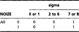
This strategy amounts to canceling out object pixels that are not on the edge. For this and a number of other algorithms (including the SHRINK and EXPAND algorithms already encountered), a thorough analysis of exactly which pixels should be set to 1 and 0 (or which should be retained and which eliminated), involves drawing up tables of the form:
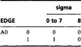
This reflects the fact that algorithm specification includes a recognition phase and an action phase. That is, it is necessary first to locate situations within an image where (for example) edges are to be marked or noise eliminated, and then action must be taken to implement the change.
Another function that can usefully be performed on binary images is the removal of “salt and pepper” noise, that is, noise that appears as a light spot on a dark background or a dark spot on a light background. The first problem to be solved is that of recognizing such noise spots; the second is the simpler one of correcting the intensity value. For the first of these tasks, the sigma value is again useful. To remove salt noise (which has binary value 0 in our convention), we arrive at the following routine:
 (2.18)
which can be read as leaving the pixel intensity unchanged unless it is proven to be a salt noise spot. The corresponding routine for removing pepper noise (binary value 1) is:
 (2.19)
Combining these two routines into one operation (Fig. 2.13a) gives:
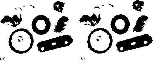
Figure 2.13 Simple binary noise removal operations: (a) result of applying a “salt and pepper” noise removal operation to the thresholded image in Fig. 2.11 b;(b) result of applying a less stringent noise removal routine: this is effective in cutting down the jagged spurs that appear on some of the objects.
 (2.20)
The routine can be made less stringent in its specification of noise pixels, so that it removes spurs on objects and background. This is achieved (Fig. 2.13b)by a variant such as
 (2.21)
As before, if any doubt about the algorithm exists, its specification should be set up rigorously—in this case with the following table:
Many other simple operations can usefully be applied to binary images, some of which are dealt with in Chapter 6. Meanwhile, we should consider the use of common logical operations such as NOT, AND, OR, EXOR. The NOT function is related to the inversion operation described earlier, in that it produces the complement of a binary image:
The other logical operations operate on two or more images to produce a third image. This may be illustrated for the AND operation:
This has the effect of masking off those parts of A-space that are not within a certain region defined in B-space (or locating those objects that are visible in both A-space and B-space).
2.2.3 Noise Suppression by Image Accumulation
The AND routine combines information from two or more images to generate a third image. It is frequently useful to average gray-scale images in a similar way in order to suppress noise. A routine for achieving this is:
This idea can be developed so that noisy images from a TV camera or other input device are progressively averaged until the noise level is low enough for useful application. It is, of course, well known that it is necessary to average 100 measurements to improve the signal-to-noise ratio by a factor of 10: that is, the signal-to-noise ratio is multiplied only by the square root of the number of measurements averaged. Since whole-image operations are computationally costly, it is usually practicable to average only up to 16 images. To achieve this the routine shown in Fig. 2.14 is applied. Note that overflow from the usual single byte per pixel storage limit will prevent this routine from working properly if the input images do not have low enough intensities. Sometimes, it may be permissible to reserve more than one byte of storage per pixel. If this is not possible, a useful technique is to employ the “learning” routine of Fig. 2.15. The action of this routine is somewhat unusual, for it retains one-sixteenth of the last image obtained from the camera and progressively lower portions of all earlier images. The effectiveness of this technique can be seen in Fig. 2.16.
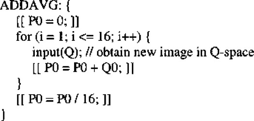
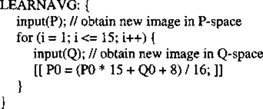
Figure 2.16 Noise suppression by averaging a number of images using the LEARNAVG routine of Fig. 2.15. Note that this is highly effective at removing much of the noise and does not introduce any blurring. (Clearly this is true only if, as here, there is no camera or object motion.) Compare this image with that of Fig. 2.1a for which no averaging was used.
Note that in this last routine 8 is added before dividing by 16 in order to offset rounding errors. If accuracy is not to suffer, this is a vital feature of most imaging routines that involve small-integer arithmetic. Surprisingly, this problem is seldom referred to in the literature, although it must account for many attempts at perfectly good algorithm strategies that mysteriously turn out not to work well in practice!
2.3 Convolutions and Point Spread Functions
Convolution is a powerful and widely used technique in image processing and other areas of science. Because it appears in many applications throughout this book, it is useful to introduce it at an early stage. We start by defining the convolution of two functions f(x) and g(x) as the integral:
The action of this integral is normally described as the result of applying a point spread function g(x) to all points of a function f(x) and accumulating the contributions at every point. It is significant that if the point spread function (PSF) is very narrow,5 then the convolution is identical to the original function f(x). This makes it natural to think of the function f(x) as having been spread out under the influence of g(x). This argument may give the impression that convolution necessarily blurs the original function, but this is not always so if, for example, the PSF has a distribution of positive and negative values.
When convolution is applied to digital images, the above formulation changes in two ways: (1) a double integral must be used in respect of the two dimensions; and (2) integration must be changed into discrete summation. The new form of the convolution is:
where g is now referred to as a spatial convolution mask. When convolutions are performed on whole images, it is usual to restrict the sizes of masks as far as possible in order to save computation. Thus, convolution masks are seldom larger than 15 pixels square, and 3 × 3 masks are typical. The fact that the mask has to be inverted before it is applied is inconvenient for visualizing the process of convolution. In this book we therefore present only preinverted masks of the form:
Convolution can then be calculated using the more intuitive formula:
Clearly, this involves multiplying corresponding values in the modified mask and the neighborhood under consideration. Reexpressing this result for a 3 × 3 neighborhood and writing the mask coefficients in the form:
the algorithm can be obtained in terms of our earlier notation:
 (2.30)
We are now in a position to apply convolution to a real situation. At this stage we merely extend the ideas of the previous section, attempting to suppress noise by averaging not over corresponding pixels of different images, but over nearby pixels in the same image. A simple way of achieving this is to use the convolution mask:
where the number in front of the mask weights all the coefficients in the mask and is inserted to ensure that applying the convolution does not alter the mean intensity in the image. As hinted earlier, this particular convolution has the effect of blurring the image as well as reducing the noise level (Fig. 2.17). More will be said about this in the next chapter.
Figure 2.17 Noise suppression by neighborhood averaging achieved by convolving the original image of Fig. 2.1a with a uniform mask within a 3 × 3 neighborhood. Note that noise is suppressed only at the expense of introducing significant blurring.
Convolutions are linear operators and are the most general spatially invariant linear operators that can be applied to a signal such as an image. Note that linearity is often of interest in that it permits mathematical analysis to be performed that would otherwise be intractable.
2.4 Sequential versus Parallel Operations
Most of the operations defined so far have started with an image in one space and finished with an image in a different space. Usually, P-space was used for an initial gray-scale image and Q-space for the processed image, or A-space and B-space for the corresponding binary images. This may seem somewhat inconvenient, since if routines are to act as interchangeable modules that can be applied in any sequence, it will be necessary to interpose restoring routines6 between modules:
Unfortunately, many of the operations cannot work satisfactorily if we do not use separate input and output spaces in this way. This is because they are inherently “parallel processing” routines. This term is used in as much as these are the types of processes that would be performed by a parallel computer possessing a number of processing elements equal to the number of pixels in the image, so that all the pixels are processed simultaneously. If a serial computer is to simulate the operation of a parallel computer, then it must have separate input and output image spaces and rigorously work in such a way that it uses the original image values to compute the output pixel values. This means that an operation such as the following cannot be an ideal parallel process:
This is so because, when the operation is half completed, the output pixel intensity will depend not only on some of the unprocessed pixel values but also on some values that have already been processed. For example, if the computer makes a normal (forward) TV raster scan through the image, the situation at a general point in the scan will be

where the ticked pixels have already been processed and the others have not. As a result, the BADSHRINK routine will shrink all objects to nothing!
A much simpler illustration is obtained by attempting to shift an image to the right using the following routine:
All this achieves is to fill up the image with values corresponding to those off its left edge,7 whatever they are assumed to be. Thus, we have shown that the BADSHIFT process is inherently parallel.
As will be seen later, some processes are inherently sequential—that is, the processed pixel has to be returned immediately to the original image space. Meanwhile, note that not all of the routines described so far need to be restricted rigorously to parallel processing. In particular, all single-pixel routines (essentially, those that only refer to the single pixel in a 1 × 1 neighborhood) can validly be performed as if they were sequential in nature. Such routines include the following inverting, intensity adjustment, contrast stretching, thresholding, and logical operations:
These remarks are intended to act as a warning. It may well be safest to design algorithms that are exclusively parallel processes unless there is a definite need to make them sequential. Later we will see how this need can arise.
2.5 Concluding Remarks
This chapter has introduced a compact notation for representing imaging operations and has demonstrated some basic parallel processing routines. The following chapter extends this work to see how noise suppression can be achieved in gray-scale images. This leads to more advanced image analysis work that is directly relevant to machine vision applications. In particular, Chapter 4 studies in more detail the thresholding of gray-scale images, building on the work of Section 2.2.1, while Chapter 6 studies object shape analysis in binary images.
Pixel-pixel operations can be used to make radical changes in digital images. However, this chapter has shown that window-pixel operations are far more powerful and capable of performing all manner of size-and-shape changing operations, as well as eliminating noise. But caveat emptor—sequential operations can have some odd effects if adventitiously applied.
2.6 Bibliographical and Historical Notes
Since this chapter seeks to provide a succinct overview of basic techniques rather than cover the most recent material, it will not be surprising that most of the topics discussed were discovered at least 20 years ago and have been used by a large number of workers in many areas. For example, thresholding of gray-scale images was first reported at least as long ago as 1960, while shrinking and expanding of binary picture objects date from a similar period. Averaging of a number of images to suppress noise has been reported many times. Although the learning routine described here has not been found in the literature, it has long been used in the author’s laboratory, and it was probably developed independently elsewhere.
Discussion of the origins of other techniques is curtailed: for further detail the reader is referred to the texts by (for example) Gonzalez and Woods (1992), Hall (1979), Jähne and Haussecker (2000), Nixon and Aguado (2002), Petrou and Bosdogianni (1999), Pratt (2001), Rosenfeld and Kak (1981), Russ (1998), and Sonka et al. (1999). More specialized texts will be referred to in the following chapters. (Note that as a matter of policy this book refers to a good many other specialized texts that have the space to delve more deeply into specific issues.) Here we refer to three texts that cover programming aspects of image processing in some depth: Parker (1994), which covers C programming; Whelan and Molloy (2001), which covers Java programming; and Batchelor (1991), which covers Prolog programming.
2.7 Problems
1. Derive an algorithm for finding the edges of binary picture objects by applying a SHRINK operation and combining the result with the original image. Is the result the same as that obtained using the edge-finding routine (2.17)? Prove your statement rigorously by drawing up suitable algorithm tables as in Section 2.2.2.
2. In a certain frame store, each off-image pixel can be taken to have either the value 0 or the intensity for the nearest image pixel. Which will give the more meaningful results for (a) shrinking, (b) expanding, and (c) blurring convolution?
3. Suppose the NOISE and NOIZE routines of Section 2.2.2 were reimplemented as sequential algorithms. Show that the action of NOISE would be unchanged, whereas NOIZE would produce very odd effects on some binary images.
1 Here we use the term channel not just to refer to the red, green, or blue channel, but any derived channel obtained by combining the colors in any way into a single color dimension.
2 Readers who are unfamiliar with C++ should refer to books such as Stroustrup (1991) and Schildt (1995).
3 The first few letters of the alphabet (A, B, C,…) are used consistently to denote binary image spaces, and later letters (P, Q, R,.) to denote gray-scale images. In software, these variables are assumed to be predeclared, and in hardware (e.g., frame store) terms they are taken to refer to dedicated memory spaces containing only the necessary 1 or 8 bits per pixel. The intricacies of data transfer between variables of different types are important considerations which are not addressed in detail here: it is sufficient to assume that both A0 = P0 and P0 = A0 correspond to a single-bit transfer, except that in the latter case the top 7 bits are assigned the value 0.
4 The processes of shrinking and expanding are also widely known by the respective terms erosion and dilation. (See also Chapter 8.)
5 Formally, it can be a delta function, which is infinite at one point and zero elsewhere while having an integral of unity.
6 Restoring is not actually necessary within a sequence of routines if the computer is able to keep track of where the currently useful images are stored and to modify the routines accordingly. Nonetheless, it can be a particular problem when it is wished to see a sequence of operations as they occur, using a frame store with only one display space.
7 Note that when the computer is performing a 3 × 3 (or larger) window operation, it has to assume some value for off-image pixel intensities. Usually, whatever value is selected will be inaccurate, and so the final processed image will contain a border that is also inaccurate. This will be so whether the off-image pixel addresses are trapped in software or in specially designed circuitry in the frame store.