
CHAPTER 5 Edge Detection
5.1 Introduction
In Chapter 4 segmentation was tackled by the general approach of finding regions of uniformity in images—on the basis that the areas found in this way would have a fair likelihood of coinciding with the surfaces and facets of objects. The most computationally efficient means of following this approach was that of thresholding, but this turns out for real images to be failure-prone or else quite difficult to implement satisfactorily. Indeed, making it work well seems to require a multiresolution or hierarchical approach, coupled with sensitive measures for obtaining suitable local thresholds. Such measures have to take account of local intensity gradients as well as pixel intensities, and the possibility of proceeding more simply—by taking account of intensity gradients alone—was suggested.
Edge detection has long been an alternative path to image segmentation, and it is the method pursued in this chapter. Whichever way is inherently the better approach, edge detection has a considerable additional advantage in that it immediately reduces by a large factor (typically around 100) the redundancy inherent in the image data. This is useful because it immensely reduces both the space needed to store the information and the amount of processing subsequently required to analyze it.
Edge detection has gone through an evolution spanning more than 30 years. Two main methods of edge detection have been apparent over this period, the first of these being template matching (TM) and the second being the differential gradient (DG) approach. In either case, the aim is to find where the intensity gradient magnitude g is sufficiently large to be taken as a reliable indicator of the edge of an object. Then g can be thresholded in a similar way to that in which intensity was thresholded in Chapter 4. (It is possible to look for local maxima of g instead of thresholding it, but this possibility and its particular complexities are ignored until a later section.) The TM and DG methods differ mainly in how they proceed to estimate g locally. However, important differences exist in how they determine local edge orientation, which is an important variable in certain object detection schemes.
5.2 Basic Theory of Edge Detection
Both DG and TM operators estimate local intensity gradients with the aid of suitable convolution masks. In the case of the DG type of operator, only two such masks are required—for the x and y directions. In the TM case, it is usual to employ up to 12 convolution masks capable of estimating local components of gradient in the different directions (Prewitt, 1970; Kirsch, 1971; Robinson, 1977; Abdou and Pratt, 1979).
In the TM approach, the local edge gradient magnitude (for short, the edge “magnitude”) is approximated by taking the maximum of the responses for the component masks:
In the DG approach, the local edge magnitude may be computed vectorially using the nonlinear transformation:
 (5.2)
(5.2)In order to save computational effort, it is common practice (Abdou and Pratt, 1979) to approximate this formula by one of the simpler forms:
or
which are, on average, equally accurate (Foglein, 1983).
In the TM approach, edge orientation is estimated simply as that of the mask giving rise to the largest value of gradient in equation (5.1). In the DG approach, it is estimated vectorially by the more complex equation:
DG equations (5.2) and (5.5) are considerably more computationally intensive than TM equation (5.1), although they are also more accurate. In some situations, however, orientation information is not required. In addition, image contrast may vary widely, so there may be little to be gained from thresholding a more accurate estimate of g. This may explain why so many workers have employed the TM instead of the DG approach. Since both approaches essentially involve estimation of local intensity gradients, it is not surprising that TM masks often turn out to be identical to DG masks—see Fig. 5.1 and 5.2.
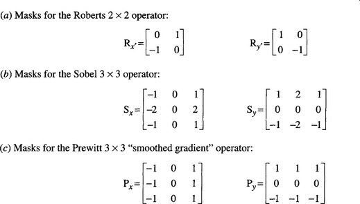
Figure 5.1 Masks of well-known differential edge operators. In this figure masks are presented in an intuitive format (viz. coefficients increasing in the positive x and y directions) by rotating the normal convolution format through 180°. This convention is employed throughout this chapter. The Roberts 2×2 operator masks (a) can be taken as being referred to axes x’, y’ at 45° to the usual x, y.
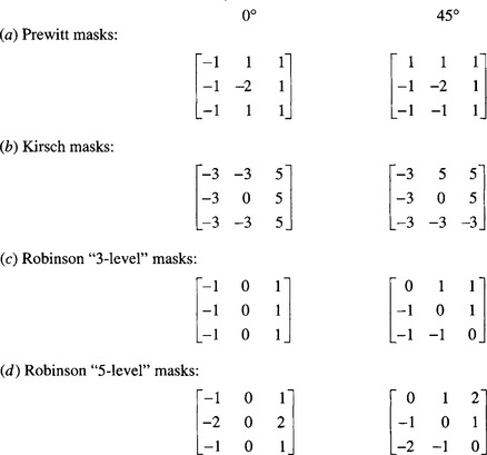
Figure 5.2 Masks of well-known 3 × 3 template matching edge operators. The figure illustrates only two of the eight masks in each set: the remaining masks can in each case be generated by symmetry operations. For the 3-level and 5-level operators, four of the eight available masks are inverted versions of the other four (see text).
5.3 The Template Matching Approach
Figure 5.2 shows four sets of well-known TM masks for edge detection. These masks were originally (Prewitt, 1970; Kirsch, 1971; Robinson, 1977) introduced on an intuitive basis, starting in two cases from the DG masks shown in Fig. 5.1. In all cases, the eight masks of each set are obtained from a given mask by permuting the mask coefficients cyclically. By symmetry, this is a good strategy for even permutations, but symmetry alone does not justify it for odd permutations. The situation is explored in more detail below.
Note first that four of the “3-level” and four of the “5-level” masks can be generated from the other four of their set by sign inversion. This means that in either case only four convolutions need to be performed at each pixel neighborhood, thereby saving computational effort. This is an obvious procedure if the basic idea of the TM approach is regarded as one of comparing intensity gradients in the eight directions. The two operators that do not employ this strategy were developed much earlier on some unknown intuitive basis.
Before proceeding, we note the rationale behind the Robinson “5-level” masks. These were intended (Robinson, 1977) to emphasize the weights of diagonal edges in order to compensate for the characteristics of the human eye, which tends to enhance vertical and horizontal lines in images. Normally, image analysis is concerned with computer interpretation of images, and an isotropic response is required. Thus, the “5-level” operator is a special-purpose one that need not be discussed further here.
These considerations show that the four template operators mentioned earlier have limited theoretical justification. It is therefore worth studying the situation in more depth, and this is done in the next section.
5.4 Theory of 3 × 3 Template Operators
Before analyzing the performance of TM operators, we note that they are likely to be used with a variety of types of edges, including in particular the “sudden step” edge, the “slanted step” edge, the “planar” edge, and various intermediate edge profiles (see Fig. 5.3). The sudden step edge has frequently been used as a paradigm with which to investigate and test the performance of edge template masks. This is highly convenient because its use eases much of the mathematical analysis, as will be seen below.
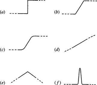
Figure 5.3 Edge models: (a) sudden step-edge; (b) slanted step edge; (c) smooth step edge; (d) planar edge; (e) roof edge; (f) line edge. The effective profiles of edge models are nonzero only within the stated neighborhood. The slanted step and the smooth step are approximations to realistic edge profiles: the sudden step and the planar edge are extreme forms that are useful for comparisons (see text). The roof and line edge models are shown for completeness only and are not considered further in this chapter.
It is assumed here that eight masks are to be used, for angles differing by 45°. In addition, four of the masks differ from the others only in sign, since this seems unlikely to result in any loss of performance. Symmetry requirements then lead to the following masks for 0° and 45°, respectively.
For a step edge, the computation devolves into a determination of the areas of various triangles and other shapes shown in Fig. 5.4. As a result, the step edge responses are computed for the 0° mask as:
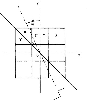
Figure 5.4 Geometry for computation of step-edge responses in a 3 × 3 neighborhood: a, angle of the step-edge; T, U, V, W, X, Y, areas of various triangles and other shapes; S, area of a single pixel (taken as unity).
 (5.7)
(5.7) (5.11)
Note that the α-axis response expressions given above are correct only for α in the range arctan(1/3) < α < arctan(1). Values for the areas V and W are given in terms of a by the expressions:
 (5.12)
and
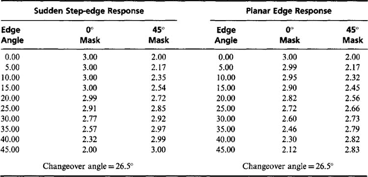
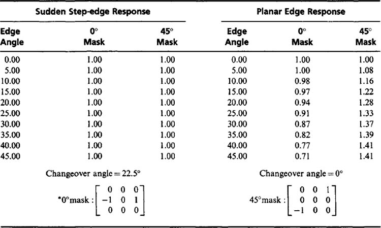
Applying these formulas to the 3-level and 5-level operators (see Fig. 5.2) immediately leads to the additional conditions A = C, B = D. Thus, the operator responses for 0° and 45° step edges are exactly equal. (It is easy to see that this is also true for the Prewitt and Kirsch operators.) This was clearly one of the original design ideas in each case. It is also possible to determine the changeover angle a at which the 0° and 45° masks give equal responses. This occurs for
which leads (for operators with A = C and B = D)to
This means that α= arctan(1/2), or 26.5°. Thus, it has been shown that 26.5° is the changeover angle for any operator of the above type in which 45° masks are generated from 0° masks merely by permuting coefficients cyclically. A more complex calculation shows that 26.5° is the changeover angle for any set of masks in which the 0° mask has reflection symmetry in the x-axis and in which the 45° mask is obtained by permuting the coefficients cyclically. This explains the fact that all four masks in Fig. 5.2 have a changeover angle of 26.5°—that is, in no case is the changeover angle equal to the ideal value of 22.5° (see, for example, Table 5.1).
As noted earlier, equalization of the respective mask response in the 0° and 45° directions was essentially one of the main specifications underlying the masks of Fig. 5.2. However, another relevant specification is that of making estimates of local edge orientation as accurate as possible: in practice, this means making the changeover angle equal to 22.5°.
To find how this affects the mask coefficients, we employ the strategy of ensuring that intensity gradients follow the rules of vector addition. If the pixel intensity values within a 3 × 3 neighborhood are

then estimation of the 0°,90°, and 45° components of gradient by the earlier general masks gives:
If vector addition is to be valid, then:
Equating coefficients of a, b, c, d, e, f, g, h, i leads to the self-consistent pair of conditions:
 (5.20)
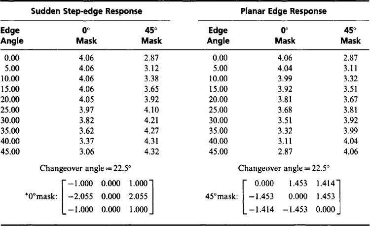
A further requirement is for the masks to give equal responses at 22.5°. This leads to the formula
 (5.22)
This gives a value for B/A in line with that for an optimized Sobel operator (see below).
The angular variations obtained with these masks are shown in Table 5.2. They are peculiar in giving optimal estimates of edge orientation for both step and planar edges and in giving relatively accurate estimates of edge magnitude for planar edges. However, their magnitude response for step edges is not particularly accurate. In this respect, it is interesting to compare the results of Table 5.1 with those of Table 5.2.
Finally, careful examination of equation (5.6)—(5.11) shows that coefficients B and D produce an isotropic contribution to the step-edge response for the 0° and 45° masks over a wide range of angles. This suggests that for greatest angular sensitivity these coefficients should be kept small, although the situation is inevitably more complicated for a planar edge. On the other hand, for least angular sensitivity, and hence greater constancy and accuracy in the estimation of edge magnitude, we may set B = D and A = C = 0. As shown in Table 5.3, this strategy works well for step edges but is not good for planar edges. Note that in the masks of Table 5.3, only two of the coefficients are nonzero, so there is very little averaging effect which can help to suppress pixel intensity noise. These considerations show clearly that a number of competing factors are involved in the design of effective edge detection operators and that it will be impossible to meet all of them with a single set of masks: hence the desired application must be specified clearly in advance.
5.5 Summary—Design Constraints and Conclusions
So far we have studied existing template masks for edge detection and examined the underlying theory. Detailed calculations have led to the design of TM operators having a variety of characteristics. At the same time, a number of design aims have become evident:
1. The need to optimize accuracy in the estimation of edge magnitude
2. The need to optimize accuracy in the estimation of edge orientation
3. The need to suppress noise during edge detection
4. The need to optimize operators for different edge profiles
These design aims have been found to conflict with each other; thus, tradeoffs between them exist and compromises have to be made. In general, it is clear (Davies, 1986a) that:
1. Different masks are needed for the accurate estimation of edge magnitude and orientation.
2. Optimization of noise suppression imposes further conditions on TM masks.
3. Obtaining sets of masks by permuting coefficients “cyclically” in a square neighborhood is ad hoc and cannot be relied upon to produce useful results.
4. The vector addition approach to the design of template masks is optimal for planar edge profiles but also gives acceptable results for step edges.
5. There is some danger in tailoring masks specifically for step-edge profiles, since they may then have poor responses for planar and other edge profiles.
Having obtained some insight into the process of designing TM masks for edge detection, we next move on to study the design of DG masks.
5.6 The Design of Differential Gradient Operators
This section studies the design of DG operators, including the Roberts 2 × 2 pixel operator and the Sobel and Prewitt 3 × 3 pixel operators (Roberts, 1965; Prewitt, 1970; for the Sobel operator see Pringle, 1969; Duda and Hart, 1973, p. 271) (see Fig. 5.1). The Prewitt or “gradient smoothing” type of operator has been extended to larger pixel neighborhoods by Prewitt (1970) and others (Brooks, 1978; Haralick, 1980) (see Fig. 5.5). In these instances the basic rationale is to model local edges by the best fitting plane over a convenient size of neighborhood. Mathematically, this amounts to obtaining suitably weighted averages to estimate slope in the x and y directions. As Haralick (1980) has pointed out, the use of equally weighted averages to measure slope in a given direction is incorrect; the proper weightings to use are given by the masks listed in Fig. 5.5. Thus, the Roberts and Prewitt operators are apparently optimal, whereas the Sobel operator is not. More will be said about this below.
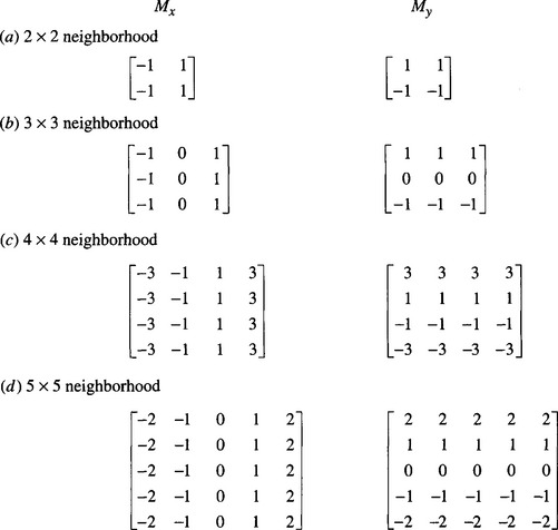
Figure 5.5 Masks for estimating components of gradient in square neighborhoods. The above masks can be regarded as extended Prewitt masks. The 3 × 3 masks are Prewitt masks, included in this table for completeness. The 2 × 2 masks can be shown to be identical to Roberts operator masks rotated through 45°. In all cases weighting factors have been omitted in the interests of simplicity, as they are throughout this chapter.
A full discussion of the edge detection problem involves consideration of the accuracy with which edge magnitude and orientation can be estimated when the local intensity pattern cannot be assumed to be planar. To analyze the situation, we again take the “worst case,” that is, that of a sudden step-edge profile, which is as distinct as possible from the planar edge approximation.
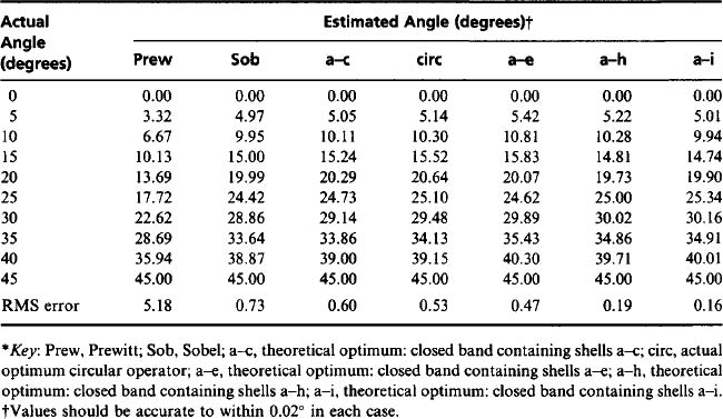
A number of analyses have been done on the angular dependencies of edge detection operators for a step-edge approximation. In particular, O’Gorman (1978) considered the variation of estimated versus actual angle resulting from a step edge observed within a square neighborhood (see also Brooks, 1978). Note that the case considered was that of a continuous rather than a discrete lattice of pixels. This was found to lead to a smooth variation, with angular error varying from zero at 0° and 45° to a maximum of 6.63° at 28.37° (where the estimated orientation was 21.74°), the variation for angles outside this range being replicated by symmetry. Abdou and Pratt (1979) obtained similar variations for the Sobel and Prewitt operators (in a discrete lattice), the respective maximum angular errors being 1.36° and 7.38° (Davies, 1984b). The Sobel operator apparently has angular accuracy that is close to optimal because it is close to being a “truly circular” operator. This point is discussed in more detail below.
5.7 The Concept of a Circular Operator
As stated earlier, when step-edge orientation is estimated in a square neighborhood, an error of up to 6.6° can result. Such an error does not arise with a planar edge approximation, since fitting of a plane to a planar edge profile within a square window can be carried out exactly. Errors appear only when the edge profile differs from the ideal planar form, within the square neighborhood—with the step-edge probably being a “worst case.”
One way to limit errors in the estimation of edge orientation might be to restrict observation of the edge to a circular neighborhood. In the continuous case, this is sufficient to reduce the error to zero for all orientations, since symmetry dictates that there is only one way of fitting a plane to a step edge within a circular neighborhood, assuming that all planes pass through the same central point. The estimated orientation 6 is then equal to the actual angle A rigorous calculation along the lines indicated by Brooks (1976), which results in the following formula for a square neighborhood (O’Gorman, 1978):
for a circular neighborhood (Davies, 1984b). Similarly, zero angular error results from fitting a plane to an edge of any profile within a circular neighborhood, in the continuous approximation. Indeed, for an edge surface of arbitrary shape, the only problem is whether the mathematical best fit plane coincides with one that is subjectively desirable (and, if not, a fixed angular correction will be required). Ignoring such cases, the basic problem is how to approximate a circular neighborhood in a digitized image of small dimensions, containing typically 3 × 3or5 × 5 pixels.
A simple way to attempt this in a 3 × 3 window might be to approximate the neighborhood by an octagon, giving the corner pixels a weight reflecting the active area of the octagon within them. A calculation of this type results in a relative corner weighting of 0.614—a value that already gives the Sobel operator significantly greater credibility. However, this approach is somewhat ad hoc and misleading. To proceed more systematically, we recall a fundamental principle stated by Haralick (1980): “[T]he fact that the slopes in two orthogonal directions determine the slope in any direction is well known in vector calculus. However, it seems not to be so well known in the image processing community.”
Essentially, appropriate estimates of slopes in two orthogonal directions permit the slope in any direction to be computed. For this principle to apply, appropriate estimates of the slopes have to be made first. If the components of slope are inappropriate, they will not act as components of true vectors, and the resulting estimates of edge orientation will be in error. This appears to be the main source of error with the Prewitt and other operators. It is not so much that the components of slope are in any instance incorrect, but rather that they are inappropriate for the purpose of vector computation since they do not match one another adequately in the required way (Davies, 1984b).
Following the arguments for the continuous case discussed earlier, slopes must be rigorously estimated within a circular neighborhood. Then the operator design problem devolves into determining how best to simulate a circular neighborhood on a discrete lattice so that errors are minimized. In order to carry this out, it is insufficient simply to weight the corner pixels after computing the masks, as implied by the octagon idea. Instead, it is necessary to apply the circular (or octagonal) weighting while computing the masks, so that correlations between the gradient weighting and circular weighting factors are taken properly into account.
5.8 Detailed Implementation of Circular Operators
In practice, the task of computing angular variations and error curves has to be tackled numerically, dividing each pixel in the neighborhood into arrays of suitably small subpixels. Each subpixel is then assigned a gradient weighting (equal to the x or y displacement) and a neighborhood weighting (equal to 1 for inside and 0 for outside a circle of radius r). The angular accuracy of “circular” differential gradient edge detection operators must depend on the radius of the circular neighborhood. In particular, poor accuracy would be expected for small values of r and reasonable accuracy for large values of r, as the discrete neighborhood approaches a continuum.
The results of this study are presented in Fig. 5.6. The variations depicted represent (1) RMS angular errors and (2) maximum angular errors in the estimation of edge orientation. The structures on each variation are surprisingly smooth. They are so closely related and systematic that they can only represent statistics of the arrangement of pixels in neighborhoods of various sizes. Details of these statistics are discussed in the next section.
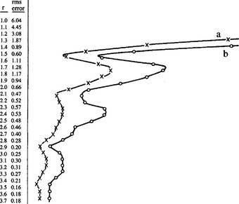
Figure 5.6 Variations in angular error as a function of radius r:(a) RMS angular error; (b) maximum angular error.
Before proceeding with a detailed interpretation of the effects depicted in Fig. 5.6, three features will be apparent. First, as expected, there is a general trend to zero angular error as r tends to infinity. This is understandable, since the discrete neighborhood is then tending toward a continuum. Second, there is a very marked periodic variation, with particularly good accuracy resulting where the circular operators best match the tessellation of the digital lattice. The third feature of interest is the fact that errors do not vanish for any finite value of r—clearly, the constraints of the problem do not permit more than the minimization of errors. Overall, these curves show that it is possible to generate a family of optimal operators (at the minima of the error curves), the first of which corresponds closely to an operator (the Sobel operator) that is known to be nearly optimal.
5.9 Structured Bands of Pixels in Neighborhoods of Various Sizes
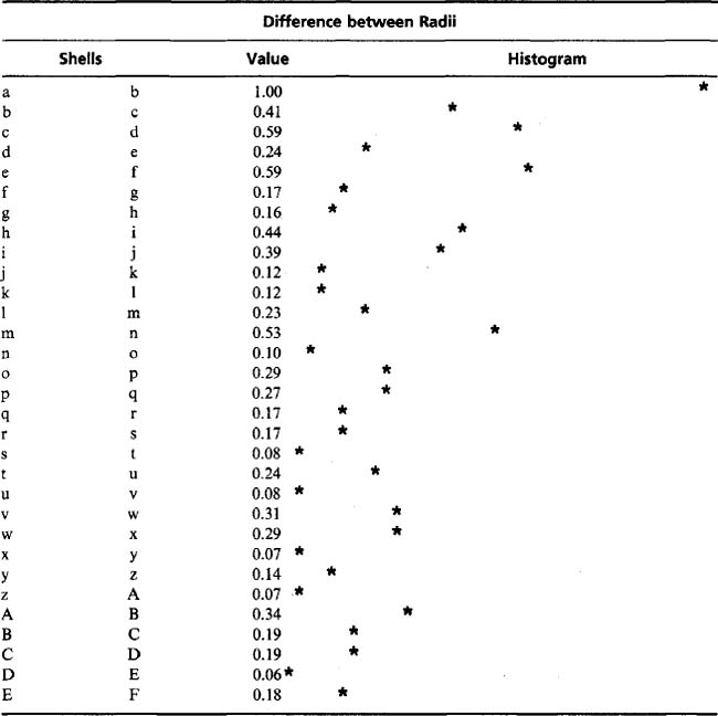
In order to explain the variations shown in Fig. 5.6, a study was made (Davies, 1984b) of the number of pixels at various distances from a given pixel, in a square lattice. Since symmetry demands that in most cases 4 or 8 pixels lie at each valid distance from the central pixel (Table 5.4), the most useful measure of the relevant statistics seems to be the difference between consecutive pixel distances. These are listed out to quite a large distance (representing neighborhoods of the order of 13 × 13) in Table 5.5. The histogram displayed in Table 5.5 indicates that a few radial differences are substantially larger than the rest. It is possible to envisage these larger values as demarcating bands of pixels which are internally well packed and approximate continua as closely as is possible. Given such continua, circular neighborhood approximations within them should be relatively accurate, whereas neighborhoods that straddle bands would be expected to be poor approximations to continua. This substantially explains the results of Fig. 5.6 and even suggests that these variations are not entirely specific to edge detection but reflect more fundamental limitations of digital image processing methodology. Thus, the design of any image processing operator should take into account banding of pixels and look for solutions that suppress pixel position statistics as far as possible.
Table 5.4 Numbers of pixels at different distances from central pixel
| Shell | Radius | No. of Pixels |
|---|---|---|
| a | 0.000 | 1 |
| b | 1.000 | 4 |
| c | 1.414 | 4 |
| d | 2.000 | 4 |
| e | 2.236 | 8 |
| f | 2.828 | 4 |
| g | 3.000 | 4 |
| h | 3.162 | 8 |
| i | 3.606 | 8 |
| j | 4.000 | 4 |
| k | 4.123 | 8 |
| l | 4.243 | 4 |
| m | 4.472 | 8 |
| n | 5.000 | 12 |
| o | 5.099 | 8 |
| p | 5.385 | 8 |
| q | 5.657 | 4 |
| r | 5.831 | 8 |
| s | 6.000 | 4 |
| t | 6.083 | 8 |
| u | 6.325 | 8 |
| v | 6.403 | 8 |
| w | 6.708 | 8 |
| x | 7.000 | 4 |
| y | 7.071 | 12 |
| z | 7.211 | 8 |
| A | 7.280 | 8 |
| B | 7.616 | 8 |
| C | 7.810 | 8 |
| D | 8.000 | 4 |
| E | 8.062 | 16 |
| F | 8.246 | 8 |
The “closed-band” operators predicted above are listed in Fig. 5.7; their angular variations appear in Table 5.6. The Sobel operator, which is already the most accurate of the 3 × 3 edge gradient operators suggested previously, can be made some 30% more accurate by adjusting its coefficients to make it more circular. In addition, the closed-bands idea indicates that the corner pixels of 5 × 5 or larger operators are best removed altogether. Not only does this require less computation but also (e.g., compared with the extended Prewitt masks of Fig. 5.5) it actually improves performance!
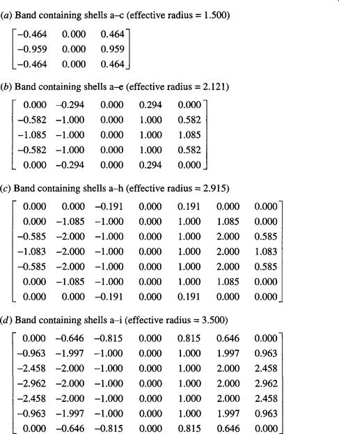
Figure 5.7 Masks of “closed band” differential gradient edge operators. In all cases only x-mask is shown: the y-mask may be obtained by a trivial symmetry operation. Mask coefficients are accurate to ~0.003 but would in normal practical applications be rounded to 1- or 2-figure accuracy.
Many sets of mask coefficients within a 3 × 3 neighborhood correspond to circular operators—that is, some value of r can be found which generates the masks in the manner outlined above. However, the Sobel operator has been shown to be more ideal in that it also corresponds approximately to a closed band situation. Since it is then closer to the ideal analog circular mask case, we may say that it is close to being a “truly circular” operator, thus justifying the statement at the end of Section 5.6. For neighborhoods larger than 3 × 3, there are so many mask coefficients that arbitrarily designed operators will not in general be “circular” or (a fortiori) “truly circular.”
The optimal 3 × 3 masks obtained above numerically by consideration of circular operators are very close indeed to those obtained purely analytically in Section 5.4, for TM masks, following the rules of vector addition. In the latter case, a value of 2.055 was obtained for the ratio of the two mask coefficients, whereas for circular operators the value 0.959/0.464 = 2.067±0.015 is obtained. This is no accident and it is very satisfying that a coefficient that was formerly regarded as ad hoc (Kittler, 1983) is in fact optimizable and can be obtained in closed form (see Section 5.4).
5.10 The Systematic Design of Differential Edge Operators
The family of “circular” differential gradient edge operators studied in Sections 5.6 -5.9 incorporates only one design parameter—the radius r. Only a limited number of values of this parameter permit optimum accuracy for estimation of edge orientation to be attained.
It is worth considering what additional properties this one parameter can control and how it should be adjusted during operator design. It affects the signal-to-noise ratio of the final edges, as well as the resolution. (These effects are important in the design of any operator, for example, in the design of an averaging filter.) The signal-to-noise ratio varies linearly with the radius of the circular neighborhood, since signal is proportional to ![]() and Gaussian noise is proportional to area, that is, to radius. This type of averaging process for improving signal-to-noise ratio is, of course, well known. Similarly, the accuracy of linear measurement is determined by the number of pixels over which averaging occurs and hence is proportional to operator radius. In contrast, resolution and the resulting “scale” of the edge image vary inversely with radius, since relevant linear properties of the image are averaged over the active area of the neighborhood. Note that the accuracy with which the positions of objects may be measured also depends on resolution. However, achievable resolution depends on available signal-to-noise ratio, and, as has been seen, this itself varies with the radius of the neighborhood. Here the final tradeoff depends on the scale of the noise one is attempting to suppress. Finally, computational load, and the associated cost of hardware for speeding up the processing, is generally at least in proportion to the number of pixels in the neighborhood, and hence in proportion to r2.
and Gaussian noise is proportional to area, that is, to radius. This type of averaging process for improving signal-to-noise ratio is, of course, well known. Similarly, the accuracy of linear measurement is determined by the number of pixels over which averaging occurs and hence is proportional to operator radius. In contrast, resolution and the resulting “scale” of the edge image vary inversely with radius, since relevant linear properties of the image are averaged over the active area of the neighborhood. Note that the accuracy with which the positions of objects may be measured also depends on resolution. However, achievable resolution depends on available signal-to-noise ratio, and, as has been seen, this itself varies with the radius of the neighborhood. Here the final tradeoff depends on the scale of the noise one is attempting to suppress. Finally, computational load, and the associated cost of hardware for speeding up the processing, is generally at least in proportion to the number of pixels in the neighborhood, and hence in proportion to r2.
These facts explain various points that appear in the literature, such as the better fidelity of the Roberts’ operator (see, for example, Bryant and Bouldin, 1979) and its higher noise levels (Abdou and Pratt, 1979). In addition, it is now seen that an exact tradeoff is operative, in that operator radius carries with it four immediate properties that have not always been seen to be intimately related: viz. signal-to-noise ratio, resolution, accuracy, and hardware/computational cost. Since none of these can be altered without the others being modified as well, one is always in an engineering situation of having to make a compromise to suit circumstances. On the other hand, the single-design parameter concept is complicated by the discreteness of the digital image processing milieu. Hence, in practice, it is necessary to fall back on one or other of the “closed-band” radii discussed above for the best combination of properties.
5.11 Problems with the Above Approach—Some Alternative Schemes
Interesting though these ideas may be, they have their own inherent problems. In particular, they take no account of the displacement E of the edge from the center of the neighborhood, or of the effects of noise in biasing the estimates of edge magnitude and orientation. Now it is possible to show that a Sobel operator gives zero error in the estimation of step-edge orientation when |θ| ≤ arctan(1/3) and |E| ≤ (cos6—3 sin|θ|)/2. For a 3 × 3 operator of the form
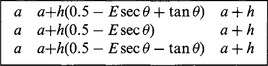
Lyvers and Mitchell (1988) found that the estimated orientation is:
which immediately shows why the Sobel operator should give zero error for a specific range of 6 and E. However, this is somewhat misleading, since considerable errors arise outside this region. Not only do they arise when E = 0, as assumed in the foregoing sections, but also they vary strongly with E. Indeed, the maximum errors for the Sobel and Prewitt operators rise to 2.90° and 7.43°, respectively, in this more general case (the corresponding RMS errors being 1.20° and 4.50°). Hence, a full analysis should be performed to determine how to reduce the maximum and average errors. Lyvers and Mitchell (1988) carried out an empirical analysis and constructed a lookup table with which to correct the orientations estimated by the Sobel operator, the maximum error being reduced to 2.06°. Their approach was motivated by the “iterated Sobel” of Iannino and Shapiro (1979).
Another scheme that reduces the error is the moment-based operator of Reeves et al. (1983). This leads to Sobel-like 3 × 3 masks that are essentially identical to the 3 × 3 masks of Davies (1984b), both having B = 2.067 (for A = 1). However, the moment method can also be used to estimate the edge position E if additional masks are used to compute second-order moments of intensity. Hence, it is possible to make a very significant improvement in performance by using a 2-D lookup table to estimate orientation: the result is that the maximum error is reduced from 2.83° to 0.135° for 3 × 3 masks and from 0.996° to 0.0042° for 5 × 5 masks.
Lyvers and Mitchell (1988) found, however, that much of this additional accuracy is lost in the presence of noise, and root mean square (RMS) standard deviations of edge orientation estimates are already around 0.5° for all 3 × 3 operators at 40 db signal-to-noise ratios. The reasons for this are quite simple. Each pixel intensity has a noise component that induces errors in its weighted mask components. The combined effects of these errors can be estimated assuming that they arise independently, so that their variances add (Davies, 1987k). Thus, noise contributions to the x and y components of gradient can be computed. These provide estimates for the components of noise along and perpendicular to the edge gradient vector (Fig. 5.8). The edge orientation for a Sobel operator is affected by an amount ![]() radians, where a is the standard deviation on the pixel intensity values and h is the edge contrast. This explains the angular errors given by Lyvers and Mitchell, if Pratt’s (2001) definition of signal-to-noise ratio (in db) is used:
radians, where a is the standard deviation on the pixel intensity values and h is the edge contrast. This explains the angular errors given by Lyvers and Mitchell, if Pratt’s (2001) definition of signal-to-noise ratio (in db) is used:
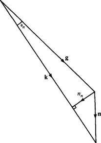
Figure 5.8 Calculating angular errors arising from noise: g, intensity gradient vector; n, noise vector; k, resultant of intensity gradient and noise vector; nn, normal component of noise; 9n, noise-induced orientation error.
An alternative approach, that of Haralick (1984), uses a “facet model” for edge detection and computes edge parameters from a polynomial surface fit at every pixel location. To estimate edge orientation accurately, a third-order model had to be used. This work was extended by Zuniga and Haralick (1987) using a special averaging technique called the integrated directional derivative (IDD). This involves integrating the directional derivative of the intensity over rectangular regions of length L and width W centered over each pixel and aligned in all possible directions 6. At any location, the edge magnitude is taken as the maximum value of the IDD, and the edge orientation as the direction that gives the maximum value. In practice, equal values of L and W have been employed—1.8 for a 5 × 5 neighborhood, 2.5 for 7 × 7. The theory permits new masks to be computed, and, indeed, application of the operator then reduces merely to application of these masks with the usual formulas for edge direction and magnitude. Under zero-noise conditions, the 5 × 5and7 × 7 operators give worst bias values of 1.05° and 0.65°, respectively. These accuracies are not quite as good as for the moment-based detectors and certainly not as good as for the moment detectors with 2-D lookup tables. However, performance in the presence of noise (S/N ratio of 30 db or worse) is virtually identical. That it is possible to obtain such improvements in edge orientation accuracy is ultimately due to the availability of many adjustable mask coefficients, though clearly suitable strategies have to be found for deducing them.
Canny (1986) developed a totally different approach. He used functional analysis to derive an optimal function for edge detection, starting with three optimization criteria—good detection, good localization, and only one response per edge under white noise conditions. The analysis is too technical to be discussed in detail here. However, the 1-D function found by Canny is accurately approximated by the derivative of a Gaussian. This is then combined with a Gaussian of identical a in the perpendicular direction, truncated at 0.001 of its peak value, and split into suitable masks. Underlying this method is the idea of locating edges at local maxima of gradient magnitude of a Gaussian-smoothed image. In addition, the Canny implementation employs a hysteresis operation (Section 7.1.1) on edge magnitude in order to make edges reasonably connected. Finally, a multiple-scale method is employed to analyze the output of the edge detector. More will be said about these points later in this chapter. Lyvers and Mitchell (1988) tested the Canny operator and found it to be significantly less accurate for orientation estimation than the moment and IDD operators. In addition, it needed to be implemented using 180 masks and hence took enormous computation time, though many practical implementations of this operator are much faster than this early paper indicates.1
Other operators have been designed for detecting edges. Of particular interest is the Hueckel approach developed in the early 1970s. This approach involved expanding intensity variations over (ideally) rather large circular regions in terms of complete sets of Fourier-like orthonormal basis functions (Hueckel, 1971, 1973). Because it is quite computationally intensive, it is not described in detail here. Suffice it to state that the tests of Lyvers and Mitchell (1988) showed that it has certain problems of convergence, especially in the presence of noise, while it involves typically 10 times the computation of other operators of comparable mask size.
An operator that has been of great historical importance is that of Marr and Hildreth (1980). The motivation for the design of this operator was the modeling of certain psychophysical processes in mammalian vision. The basic rationale is to find the Laplacian of the Gaussian-smoothed (∇2G) image and then to obtain a “raw primal sketch” as a set of zero-crossing lines. The Marr—Hildreth operator does not use any form of threshold since it merely assesses where the ∇2G image passes through zero. This feature is attractive, for working out threshold values is a difficult and unreliable task. However, the Gaussian smoothing procedure can be applied at a variety of scales, and in one sense the scale is a new parameter that substitutes for the threshold. In fact, a major feature of the Marr—Hildreth approach that has been very influential in later work (Witkin, 1983; Bergholm, 1986) is the fact that zero-crossings can be obtained at several scales, giving the potential for more powerful semantic processing. This necessitates finding the means to combine all the information in a systematic and meaningful way. This may be carried out by bottom-up or top-down approaches, and there is much discussion in the literature about methods for carrying out these processes. However, in many (especially industrial inspection) applications, one is interested in working at a particular resolution, and considerable savings in computation can then be made. It is also noteworthy that the Marr—Hildreth operator is reputed to require neighborhoods of at least 35 × 35 for proper implementation (Brady, 1982). Nevertheless, other workers have implemented the operator in much smaller neighborhoods, down to 5 × 5. Wiejak et al. (1985) showed how to implement the operator using linear smoothing operations to save computation. Lyvers and Mitchell (1988) reported orientation accuracies using the Marr—Hildreth operator that are not especially high (2.47° for a 5 × 5 operator and 0.912° for a 7 × 7 operator, in the absence of noise).
As noted earlier, those edge detection operators that are applied at different scales lead to different edge maps at different scales. In such cases, certain edges that are present at lower scales disappear at larger scales; in addition, edges that are present at both low and high scales may be shifted or merged at higher scales. Bergholm (1986) demonstrated the possible occurrence of elimination, shifting, and merging, while Yuille and Poggio (1986) showed that edges that are present at high resolution should not disappear at some lower resolution. These aspects of edge location are now becoming well understood.
Finally, Overington and Greenway (1987) sound a cautionary note about the accuracy of the zero-crossing approach to edge detection. They found that it is significantly more accurate to estimate edge position and edge orientation by interpolating to local maximum values of edge gradient than by locating zero-crossings of the ∇2G image. Their rationale was that accurate estimation of these zero-crossing positions relies on third derivatives of the image intensity function, which tend to be affected seriously by noise.
5.12 Concluding Remarks
The design of edge detection operators has by now been taken to quite an advanced stage, so that edges can be located to subpixel accuracy and orientated to fractions of a degree. In addition, edge maps may be made at several scales and the results correlated as an aid to image interpretation. Unfortunately, some of the schemes that have been devised to achieve these things (and especially those outlined in the previous section) are fairly complex and tend to consume considerable computation. In many applications, this complexity may not be justified because the application requirements are, or can reasonably be made, quite restricted. Furthermore, there is often the need to save computation for realtime implementation. For these reasons, the remainder of this book reverts to employing edges found by a single low-resolution detector. In practice, this will normally be a Sobel operator, which provides a good balance between computational load and orientation accuracy. Indeed, virtually all the examples in Part 2 of the book have been implemented using a Sobel operator. (In addition, the RMS error in estimating edge orientation using this operator was found by Lyvers and Mitchell to be 1.20°, and in later chapters this quantity will generally be taken as a round 1 °.) This does not in any way invalidate the latest methods, particularly those involving studies of edges at various scales. Such methods come into their own in applications such as general scene analysis, where vision systems are required to cope with largely unconstrained image data.
This chapter has largely completed the task of segmentation of images at low level. The following chapter moves on to consider the shapes of objects that have been found by the thresholding and edge detection schemes discussed in the last two chapters. In fact, Chapter 6 studies shapes by analysis of the regions over which objects extend, while Chapter 7 studies shapes by considering their boundary patterns.
Edge detection is perhaps the most widely used means of locating and identifying objects in digital images. While different edge detection strategies vie with each other for acceptance, this chapter has shown that all obey fundamental laws—such as sensitivity, noise suppression capability, and computation cost all increasing with footprint size.
5.13 Bibliographical and Historical Notes
Early attempts at edge detection tended to employ numbers of template masks that could locate edges at various orientations. Often these masks were ad hoc in nature, and after 1980 this approach finally gave way to the differential gradient approach that had already existed in various forms for a considerable period (see the influential paper by Haralick, 1980).
The Frei—Chen approach is of particular interest in that it takes a set of nine 3 × 3 masks forming a complete set within this size of neighborhood—of which one tests for brightness, four test for edges, and four test for lines (Frei and Chen, 1977). Though interesting, the Frei—Chen edge masks do not correspond to those devised for optimal edge detection, and it appears possible that edge detection in the set as a whole may have been compromised in some way in order to make a complete “toolbox.” Indeed, Lacroix (1988) found errors in the Frei—Chen approach which may ultimately show how to rationalize the situation.
The Hueckel scheme (1971, 1973) provided an early alternative to these approaches, although it was rather computationally intensive and therefore perhaps not so widely used. To tackle this problem, Mero and Vassy (1975) developed a modified form of the scheme, but it does not appear to have been used particularly widely.
Meanwhile, psychophysical work by Marr (1976), Wilson and Giese (1977), and others provided another line of development for edge detection. This led to the well-known paper by Marr and Hildreth (1980), which was highly influential in the following few years. This spurred others to think of alternative schemes, and the Canny (1986) operator emerged from this vigorous milieu. The Marr—Hildreth operator seems to have been the first to preprocess images in order to study them at different scales—a technique that has survived and expanded considerably (see for example, Witkin, 1983; Bergholm, 1986; Yuille and Poggio, 1986). The computational problems of the Marr—Hildreth operator have kept others thinking along more traditional lines, and the work by Reeves et al. (1983), Haralick (1984), and Zuniga and Haralick (1987) falls into this category. Lyvers and Mitchell (1988) reviewed many of these papers and made their own suggestions. Other studies (McIvor, 1988; Petrou and Kittler, 1988) show continuing development in the subject, especially regarding operator optimization, although it is not improbable that diminishing returns have now set in and that from now on the main advances will be at a higher level. In this context, the work of Sjoberg and Bergholm (1988), which finds rules for discerning shadow edges from object edges, is of great interest. Nevertheless, other nuances are worth considering, such as the accuracy of edge orientation for partly saturated gray-scale images (Davies and Celano, 1993a), and the development of edge detectors that are suited to particular purposes, such as finding high accuracy subedges for use in conjunction with a Hough transform (Davies, 1992c).
Most recently, there has been a move to achieve greater robustness and confidence in edge detection by careful elimination of local outliers. In Meer and Georgescu’s (2001) method, this is achieved by estimating the gradient vector, suppressing nonmaxima, performing hysteresis thresholding (Section 7.1.1), and integrating with a confidence measure to produce a more general robust result. Each pixel is assigned a confidence value before the final two steps of the algorithm. Kim et al. (2004) have taken this technique a step further and eliminated the need for setting a threshold by using a fuzzy reasoning approach. Yitzhaky and Peli (2003) have expressed similar sentiments and they aim to find an optimal parameter set for edge detectors by ROC and chi-square measures, which actually give very similar results. Prieto and Allen (2003) designed a similarity metric for edge images, which could be used to test the effectiveness of a variety of edge detectors. They pointed out that metrics need to allow slight latitude in the positions of edges, in order to compare the similarity of edges reliably. They report a new approach that takes into account not only displacement of edge positions but also edge strengths in determining the similarity between edge images.
Not content with handcrafted algorithms, Suzuki et al. (2003) devised a backpropagation neural edge enhancer that undergoes supervised learning on model data to permit it to cope well (in the sense of giving clear, continuous edges) with noisy images. It was found to give results superior to those of conventional algorithms (including Canny, Heuckel, Sobel, and Marr-Hildreth) in similarity tests relative to the desired edges. The disadvantage was a long learning time, though the final execution time was short.
Finally, Cheng (2003) produced a rapidly operating moment-preserving edge detector working in image blocks in order to facilitate fast image database searches for likely image structures without the need for special hardware. This is a use for which increasing speed will be demanded for the foreseeable future, regardless of computer speeds, as more and more images and image sequences have to be searched. However, the method presented cannot be described as a temporary expedient “fix,” as its results seem impressive and yield exactly the type of data needed in such applications.
5.14 Problems
1. Prove equation (5.22) and (equation 5.23).
2. Check the results quoted in Section 5.11 giving the conditions under which the Sobel operator leads to zero error in the estimation of edge orientation. Proceed to prove equation (5.26).
1 It is nowadays necessary to ask “Which Canny?”, as there are a great many implementations of it: this leads to problems for any realistic comparison between operators.