17.1 Introduction

This chapter tackles a problem of central importance in the analysis of images from 3-D scenes. It has been kept separate and fairly short so as to focus carefully on relevant factors in the analysis. First, we look closely at the phenomenon of perspective inversion, which has already been alluded to several times in Chapter 16. Then we refine our ideas on perspective and proceed to consider the determination of object pose from salient features which are located in the images. It will be of interest to consider how many salient features are required for unambiguous determination of pose.

17.2 The Phenomenon of Perspective Inversion

In this section, we first study the phenomenon of perspective inversion. This is actually a rather well-known effect that appears in the following “Necker cube” illusion. Consider a wire cube made from 12 pieces of wire welded together at the corners. Looking at it from approximately the direction of one corner, we have a difficult time telling which way round the cube is, that is, which of the opposite corners of the cube is the nearer (Fig. 17.1). On looking at the cube for a time, one gradually comes to feel one knows which way round it is, but then it suddenly appears to reverse itself. Then that perception remains for some time, until it, too, reverses itself.¹ This illusion reflects the fact that the brain is making various hypotheses about the scene, and even making decisions based on incomplete evidence about the situation (Gregory, 1971, 1972).

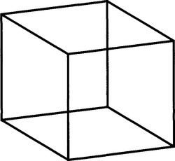
Figure 17.1 The phenomenon of perspective inversion. This figure shows a wire cube viewed approximately from the direction of one corner. The phenomenon of perspective inversion makes it difficult to see which of the opposite corners of the cube is the nearer. There are two stable interpretations of the cube, either of which may be perceived at any moment.

The wire cube illusion could perhaps be regarded as somewhat artificial. But consider instead an airplane (Fig. 17.2a) which is seen in the distance (Fig. 17.2b) against a bright sky. The silhouetting of the object means that its surface details are not visible. In that case, interpretation requires that a hypothesis be made about the scene, and it is possible to make the wrong one. Clearly (Fig. 17.2c), the airplane could be at an angle αψ (as for P), though it could equally well be at an angle −αψ (as for Q). The two hypotheses about the orientation of the object are related by the fact that the one can be obtained from the other by reflection in a plane R normal to the viewing direction D.

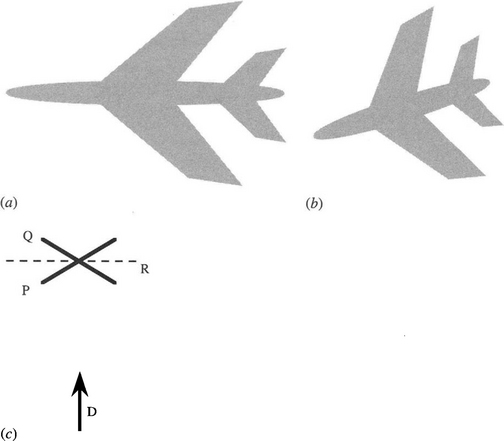
Figure 17.2 Perspective inversion for an airplane. Here an airplane (a) is silhouetted against the sky and appears as in (b). (c) shows the two planes P and Q in which the airplane could lie, relative to the direction D of viewing: R is the reflection plane relating the planes P and Q.

Strictly, there is only an ambiguity in this case if the object is viewed under orthographic or scaled orthographic projection.² However, in the distance, perspective projection approximates to scaled orthographic projection, and it is often difficult to detect the difference.³ If the airplane in Fig. 17.2 were quite near, it would be obvious that one part of the silhouette was nearer, as the perspective would distort it in a particular way. In general, perspective projection will break down symmetries, so searching for symmetries that are known to be present in the object should reveal which way around it is. However, if the object is in the distance, as in Fig. 17.2b, it will be virtually impossible to see the breakdown. Unfortunately, short-term study of the motion of the airplane will not help with interpretation in the case shown in Fig. 17.2b. Eventually, however, the airplane will appear to become smaller or larger, which will give the additional information needed to resolve the issue.

17.3 Ambiguity of Pose under Weak Perspective Projection

It is instructive to examine to what extent the pose of an object can be deduced under weak perspective projection. We can reduce the above problem to a simple case in which three points have to be located and identified. Any set of three points is coplanar, and the common plane corresponds to that of the silhouette shown in Fig. 17.2a.(We assume here that the three points are not collinear, so that they do in fact define a plane.) The problem then is to match the corresponding points on the idealized object (Fig. 17.2a) with those on the observed object (Fig. 17.2b). It is not yet completely obvious that this is possible or that the solution is unique, even apart from the reflection operation noted earlier. It could be that more than three points will be required—especially if the scale is unknown—or it could be that there are several solutions, even if we ignore the reflection ambiguity. Of particular interest will be the extent to which it is possible to deduce which is which of the three points in the observed image.

To understand the degree of difficulty, let us briefly consider full perspective projection. In this case, any set of three noncollinear points can be mapped into any other three. This means that it may not be possible to deduce much about the original object just from this information. We will certainly not be able to deduce which point maps to which other point. However, we shall see that the situation is rather less ambiguous when we view the object under weak perspective projection.

Perhaps the simplest approach (due to Huang, et al. as recently as 1995) is to imagine a circle drawn through the original set of points P₁,P₂,P₃ (Fig. 17.3a). We then find the centroid C of the set of points and draw additional lines through the points, all passing through C and meeting the circle in another three points Q₁,Q₂,Q₃ (Fig. 17.3a). Now in common with orthographic projection, scaled orthographic projection maintains ratios of distances on the same straight line, and weak perspective projection approximates to this. Thus, the distance ratio P_iC:CQ_i remains unchanged after projection, and when we project the whole figure, as in Fig. 17.3b, we find that the circle has become an ellipse, though all lines remain lines and all linear distance ratios remain unchanged. The significance of these transformations and invariances is as follows. When the points P’₁,P’₂,P’₃ are observed in the image, the centroid C’ can be computed, as can the positions of Q’₁,Q’₂,Q’₃. Thus, we have six points by which to deduce the position and parameters of the ellipse (in fact, five are sufficient). Once the ellipse is known, the orientation of its major axis gives the axis of rotation of the object; whereas the ratio of the lengths of the minor to major axes immediately gives the value of cos α. (Notice how the ambiguity in the sign of αψ comes up naturally in this calculation.) Finally, the length of the major axis of the ellipse permits us to deduce the depth of the object in the scene.

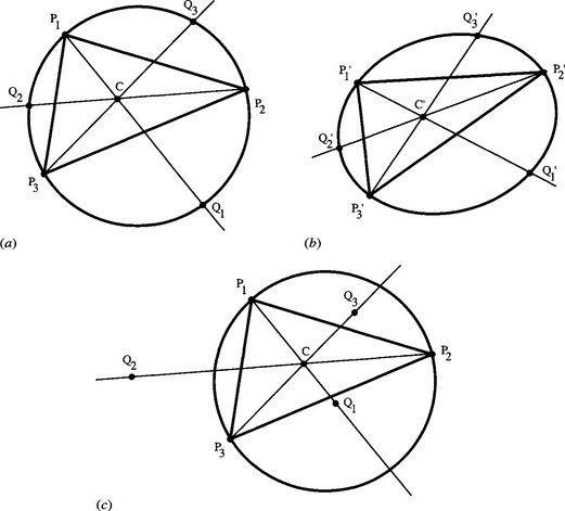
Figure 17.3 Determination of pose for three points viewed under weak perspective projection. (a) shows three feature points P1,P2,P3 which lie on a known type of object. The circle passing through P₁,P₂,P₃ is drawn, and lines through the points and their centroid C meet the circle in Q₁,Q₂,Q₃. The ratios P_iC: CQ_i are then deduced. (b) shows the three points observed under weak perspective as P’₁,P’₂, P’₃, together with their centroid C’ and the three points Q’₁,Q’₂,Q’₃ located using the original distance ratios. An ellipse drawn through the six points P’₁,P’₂,P’₃,Q’₁,Q’₂,Q’₃ can now be used to determine the orientation of the plane in which P₁,P₂,P₃ must lie, and also (from the major axis of the ellipse) the distance of viewing. (c) shows how an erroneous interpretation of the three points does not permit a circle to be drawn passing through P₁,P₂,P₃,Q₁,Q₂,Q₃ and hence no ellipse can be found which passes through the observed and the derived points P’₁,P’₂,P’₃,Q’₁,Q’₂,Q’₃.

We have now shown that observing three projected points permits a unique ellipse to be computed passing through them. When this is back-projected into a circle, the axis of rotation of the object and the angle of rotation can be deduced, but not the sign of the angle of rotation. Two important comments may be made about the above calculation. The first is that the three distance ratios must be stored in memory, before interpretation of the observed scene can begin. The second is that the order of the three points apparently has to be known before interpretation can be undertaken. Otherwise we will have to perform six computations in which all possible assignments of the distance ratios are tried. Furthermore, it might appear from the earlier introductory remarks that several solutions are possible. Although in some instances feature points might be distinguishable, in many cases they are not (especially in 3-D situations where corner features might vary considerably when viewed from different positions). Thus, the potential ambiguity is important. However, if we can try out each of the six cases, little difficulty will generally arise. For immediately we deduce the positions Q’₁,Q’₂,Q’₃,we will find that it is not possible in general to fit the six resulting points to an ellipse. The reason is easily seen on returning to the original circle. In that case, if the wrong distance ratios are assigned, the Q_i will clearly not lie on the circle, since the only values of the distance ratios for which the Q_i do lie on the circle are the correctly assigned ones (Fig. 17.3c). This means that although computation is wasted testing the incorrect assignments, there appears to be no risk of their leading to ambiguous solutions. Nevertheless, there is one contingency under which things could go wrong. Suppose the original set of points P1,P2,P3 forms an almost perfect equilateral triangle. Then the distance ratios will be very similar, and, taking numerical inaccuracies into account, it may not be clear which ellipse provides the best and most likely fit. This mitigates against taking sets of feature points that form approximately isosceles or equilateral triangles. However, in practice more than three coplanar points will generally be used to optimize the fit, making fortuitous solutions rather unlikely.

Overall, it is fortunate that weak perspective projection requires such weak conditions for the identification of unique (to within a reflection) solutions, especially as full perspective projection demands four points before a unique solution can be found (see below). However, under weak perspective projection, additional points lead to greater accuracy but no reduction in the reflection ambiguity. This is because the information content from weak perspective projection is impoverished in the lack of depth cues that could (at least in principle) resolve the ambiguity. To understand this lack of additional information from more than three points under weak perspective projection, note that each additional feature point in the same plane is predetermined once three points have been identified. (Here we are assuming that the model object with the correct distance ratios can be referred to.)

These considerations indicate that we have two potential routes to unique location of objects from limited numbers of feature points. The first is to use noncoplanar points still viewed under weak perspective projection. The second is to use full perspective projection to view coplanar or noncoplanar sets of feature points. We shall see that whichever of these options we take, a unique solution demands that a minimum of four feature points be located on any object.

17.4 Obtaining Unique Solutions to the Pose Problem

The overall situation is summarized in Table 17.1. Looking first at the case of weak perspective projection (WPP), the number of solutions only becomes finite for three or more point features. Once three points have been employed, in the coplanar case there is no further reduction in the number of solutions, since (as noted earlier) the positions of any additional points can be deduced from the existing ones. However, this does not apply when the additional points are noncoplanar since they are able to provide just the right information to eliminate any ambiguity (see Fig. 17.4). (Although this might appear to contradict what was said earlier about perspective inversion, note that we are assuming here that the body is rigid and that all its features are at known fixed points on it in three dimensions. Hence, this particular ambiguity no longer applies, except for objects with special symmetries which we shall ignore here—see Fig. 17.4d.)

Table 17.1 Ambiguities when estimating pose from point features

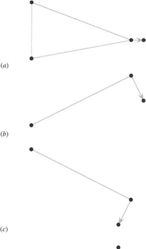
Figure 17.4 Determination of pose for four points viewed under weak perspective projection. (a) shows an object containing four noncoplanar points, as seen under weak perspective projection. (b) shows a side view of the object. If the first three points (connected by nonarrowed gray lines) were viewed alone, perspective inversion would give rise to a second interpretation (c). However, the fourth point gives additional information about the pose, which permits only one overall interpretation. This would not be the case for an object containing an additional symmetry as in (d), since its reflection would be identical to the original view (not shown).

Considering next the case of full perspective projection (FPP), we find that the number of solutions again becomes finite only for three or more point features. The lack of information provided by three point features means that four solutions are in principle possible (see the example in Fig. 17.5 and the detailed explanation in Section 17.2.1), but the number of solutions drops to one as soon as four coplanar points are employed. (The correct solution can be found by making cross checks between subsets of three points, and eliminating inconsistent solutions.) When the points are noncoplanar, it is only when six or more points are employed that we have sufficient information to unambiguously determine the pose. There is necessarily no ambiguity with 6 or more points, as all 11 camera calibration parameters can be deduced from the 12 linear equations that then arise (see Chapter 21). Correspondingly, it is deduced that 5 noncoplanar points will in general be insufficient for all 11 parameters to be deduced, so there will still be some ambiguity in this case.

Figure 17.5 Ambiguity for three points viewed under full perspective projection. Under full perspective projection, the camera sees three points A, B, C as three directions in space, and this can lead to a fourfold ambiguity in interpreting a known object. The figure shows the four possible viewing directions and centers of projection of the camera (indicated by the directions and tips of the bold arrows). In each case, the image at each camera is indicated by a small triangle. D_A,D_B,D_C correspond approximately to views from the general directions of A, B, C, respectively.

Next, it should be questioned why the coplanar case is at first (N = 3) better⁴ under weak perspective projection and then (N > 3) better under full perspective projection, although the noncoplanar case is always better, or as good, under weak perspective projection. The reason must be that intrinsically full perspective projection provides more detailed information but is frustrated by lack of data when there are relatively few points. However, the exact stage at which the additional information becomes available is different in the coplanar and noncoplanar cases. In this respect, it is important to note that when coplanar points are being observed under weak perspective projection there is never enough information to eliminate the ambiguity.

Our discussion assumes that the correspondences between object and image features are all known—that is, that N point features are detected and identified correctly and in the correct order. If this is not so, the number of possible solutions could increase substantially, considering the number of possible permutations of quite small numbers of points. This makes it attractive to use the minimum number of features for ascertaining the most probable match (Horaud et al., 1989). Other workers have used heuristics to help reduce the number of possibilities. For example, Tan (1995) used a simple compactness measure (see Section 6.9) to determine which geometric solution is the most likely. Extreme obliqueness is perhaps unlikely, and the most likely solution is taken to be the one with the highest compactness value. This idea follows on from the extremum principle of Brady and Yuille (1984), which states that the most probable solutions are those nearest to extrema of relevant (e.g., rotation) parameters.⁵ In this context, it is worth noting that coplanar points viewed under weak or full perspective projection always appear in the same cyclic order. This is not trivial to check given the possible distortions of an object, though if a convex polygon can be drawn through the points, the cyclic order around its boundary will not change on projection.⁶ However, for noncoplanar points, the pattern of the perceived points can reorder itself almost randomly. Thus, a considerably greater number of permutations of the points have to be considered for noncoplanar points than for coplanar points.

Finally, to this point we have concentrated on the existence and uniqueness of solutions to the pose problem. The stability of the solutions has not so far been discussed. However, the concept of stability gives a totally different dimension to the data presented in Table 17.1. In particular, noncoplanar points tend to give more stable solutions to the pose problem. For example, if the plane containing a set of coplanar points is viewed almost head-on (α ≈ 0), there will be very little information on the exact orientation of the plane because the changes in lateral displacement ofthe points will vary as cos α (see Section 17.1) and there will be no linear term in the Taylor expansion of the orientation dependence.

17.4.2 Using Symmetrical Trapezia for Estimating Pose

One more example will be of interest here. That is the case of four points arranged at the corners of a symmetrical trapezium (Tan, 1995). When viewed under weak perspective projection, the midpoints of the parallel sides are easily measured, but under full perspective projection midpoints do not remain midpoints, so the axis of symmetry cannot be obtained in this way. However, producing the skewed sides to meet at S’ and forming the intersection I⁰ of the diagonals permit the axis of symmetry to be located as the line I’S’ (Fig. 17.6). Thus, we now have not four points but six to describe the perspective view of the trapezium. More important, the axis of symmetry has been located, and this is known to be perpendicular to the parallel sides of the trapezium. This fact is a great help in making the mathematics more tractable and in obtaining solutions quickly so that (for example) object motion can be tracked in real time. Again, this is a case where object orientation can be deduced straightforwardly, even when the situation is one of strong perspective and even when the size of the object is unknown. This result is a generalization from that of Haralick (1989) who noted that a single view of a rectangle of unknown size is sufficient to determine its pose. In either case, the range of the object can be found if its area is known, or its size can be deduced if a single range value can be found from other data (see also Section 17.3.1).

Figure 17.6 Trapezium viewed under full perspective projection. (a) shows a symmetrical trapezium, and (b) shows how it appears when viewed under full perspective projection. In spite of the fact that midpoints do not project into midpoints under perspective projection, the two points S’ and I’ on the symmetry axis can be located unambiguously as the intersection of two nonparallel sides and two diagonals respectively. This gives six points (from which the two midpoints on the symmetry axis can be deduced if necessary), which is sufficient to compute the pose of the object, albeit with a single ambiguity of interpretation (see text).

17.5 Concluding Remarks

This chapter has aimed to cover certain aspects of 3-D vision that were not studied in depth in the previous chapter. In particular, the topic of perspective inversion was investigated in some detail, and its method of projection was explored. Orthographic projection, scaled orthographic projection, weak perspective projection, and full perspective projection were considered, and the numbers of object points that would lead to correct or ambiguous interpretations were analyzed. It was found that scaled orthographic projection and its approximation, weak perspective projection, led to straightforward interpretation when four or more noncoplanar points were considered, although the perspective inversion ambiguity remained when all the points were coplanar. This latter ambiguity was resolved with four or more points viewed under full perspective projection. However, in the noncoplanar case, some ambiguity remained until six points were being viewed. The key to understanding the situation is the fact that full perspective projection makes the situation more complex, although it also provides more information by which, ultimately, to resolve the ambiguity.

Additional problems were found to arise when the points being viewed are indistinguishable and then a good many solutions may have to be tried before a minimally ambiguous result is obtained. With coplanar points fewer possibilities arise, which leads to less computational complexity. The key to success here is the natural ordering that can arise for points in a plane—as, for example, when they form a convex set that can be ordered uniquely around a bounding polygon. In this context, the role that can be played by the extremum principle of Brady and Yuille (1984) in reducing the number of solutions is significant. (For further insight on the topic, see Horaud and Brady, 1988.)

It is of great relevance to devise methods for rapid interpretation in real-time applications. To do so it is important to work with a minimal set of points and to obtain analytic solutions that move directly to solutions without computationally expensive iterative procedures: for example, Horaud et al. (1989) found an analytic solution for the perspective four-point problem, which works both in the general noncoplanar case and in the planar case. Other low computation methods are still being developed, as with pose determination for symmetrical trapezia (Tan, 1995). Understanding is still advancing, as demonstrated by Huang, et al.’s (1995) neat geometrical solution to the pose determination problem for three points viewed under weak perspective projection.

This chapter has covered a specific 3-D recognition problem. Chapter 19 covers another—that of invariants, which provides a speedy and convenient means of bypassing the difficulties associated with full perspective projection. Chapter 21 aims to finalize the study of 3-D vision by showing how camera calibration can be achieved or, to some extent, circumvented.

17.6 Bibliographical and Historical Notes

The development of solutions to the so-called perspective n-point problem (finding the pose of objects from n features under various forms of perspective) has been proceeding for more than two decades and is by no means complete. Fischler and Bolles summarized the situation as they saw it in 1981, and they described several new algorithms. However, they did not discuss pose determination under weak perspective, and perhaps surprisingly, considering its reduced complexity, pose determination under weak perspective has subsequently been the subject of much research (e.g., Alter, 1994; Huang et al., 1995). Horaud et al. (1989) discussed the problem of finding rapid solutions to the perspective n-point problem by reducing n as far as possible. They also obtained an analytic solution for the case n = 4, which should help considerably with real-time implementations. Their solution is related to Horaud’s earlier (1987) corner interpretation scheme, as described in Section 16.12, while Haralick et al. (1984) provided useful basic theory for matching wire frame objects.

In a recent paper, Liu and Wong (1999) described an algorithm for pose estimation from four corresponding points under FPP when the points are not coplanar. Strictly, according to Table 17.1, this will lead to an ambiguity. However, Liu and Wong made the point “that the possibility for the occurrence of multiple solutions in the perspective 4-point problem is much smaller than that in the perspective 3-point problem,” so that “using a 4-point model is much more reliable than using a 3-point model.” They actually only claim “good results.” Also, much of the emphasis of the paper is on errors and reliability. Hence, it seems that it is the scope for making errors in the sense ofmisinterpreting the situation that is significantly reduced. Added to this consideration, Liu and Wong’s (1999) work involves tracking a known object within a somewhat restricted region of space. This must again cut down the scope for error considerably. Hence, it is not clear that their work violates the relevant (FPP; noncoplanar; n = 4)⁷ entry in Table 17.1, rather than merely making it unlikely that a real ambiguity will arise.

Between them, Faugeras (1993), Hartley and Zisserman (2000), Faugeras and Luong (2001), and Forsyth and Ponce (2003) provide good coverage of the whole area of 3-D vision. For an interesting viewpoint on the subject, with particular emphasis on pose refinement, see Sullivan (1992). For further references on specific aspects of 3-D vision, see Sections 16.15, 19.8, and 21.16. (Sections 18.15 and 20.12 give references on motion but also cover aspects of 3-D vision.)

17.7 Problems

Figure 17.P1 In this diagram the gray edges are construction lines, not parts of the objects. (a) and (b) are completely planar objects.